Influence of external phase and gain-loss
modulation on bound solitons in laser systems
Wonkeun Chang,1,*Nail Akhmediev,1Stefan Wabnitz,2and Majid Taki3 1
Optical Sciences Group, Research School of Physics and Engineering, The Australian National University, Canberra, Australian Capital Territory 0200, Australia
2
Dipartimento di Elettronica per l’Automazione, University of Brescia, Via Branze 38, 25123 Brescia, Italy 3
Laboratoire de Physique des Lasers, Atomes et Molécules, UMR-CNRS 8523 IRCICA, Université des Sciences et Technologies de Lille, 59655 Villeneuve d’Ascq CEDEX, France
*Corresponding author: [email protected]
Received August 10, 2009; revised September 23, 2009; accepted September 23, 2009; published October 30, 2009 We study the dynamics of bound solitons of the complex cubic-quintic Ginzburg– Landau equation under the influence of external modulation. We consider periods of modulation being either smaller or larger than the soliton separation and the amplitude of modulation being either real or imaginary. For each case, we observe bifurcation and hysteresis phenomena in the parameters of the pair when changing the amplitude of modula-tion. Namely, soliton separation and phase difference between the solitons may take two or more values for the same modulation amplitude. In the case of gain-loss modulation, two solitons may split and be positioned in the two equilibrium states of the periodic potential. The complicated dynamics of this process is illustrated with numerical examples. © 2009 Optical Society of America
OCIS codes: 140.4050, 190.0190.
1. INTRODUCTION
One of the ways of generating pulses out of laser oscilla-tors rather than continuous waves (CWs) is the passive mode-locking technique [1–4]. This technique uses the transmission characteristics of the cavity that depend on the intensity of optical radiation. In this way, the insta-bility of the CW regime of operation drives the laser into pulsations. There is a variety of ways to obtain a nonlin-ear transmission: each method has its own advantages and disadvantages [5–8]. The main advantage of passive mode locking is that pulses are generated in a self-organized way by taking the form of dissipative solitons [9,10].
External phase [11] or gain-loss modulation is another efficient way of pulse generation in laser cavities [12–19]. This technique is well known as active mode locking. Ap-plication of an external periodic modulation with a well-defined temporal period allows for the generation of a se-quence of pulses with a given separation between them.
An interesting and relatively less explored possibility is the combination of both passive and active mode-locking mechanisms in a sort of hybrid mode locking [20]. Pulses or pulse pairs may already appear in the cavity due to the passive mode-locking mechanism. On the other hand, their exact location inside the round trip is defined by the active mode locking. In this way, pulse generation pro-cesses may be controlled more efficiently, thus, providing us with versatile optical tools. Although there are a num-ber of experimental works [18–21] demonstrating this technique, the full understanding of the effect of the modulating process in determining the properties of the generated pulses is far from being reached. Passive mode locking provides favorable conditions for pulse emission, while active mode locking modifies their shape or time
lo-cation. As mentioned, there are two different techniques for active mode locking. In the first one, the optical length of the cavity is modulated by using the change in the re-fractive index of a crystal inside the cavity. In the second case, the gain or loss in the cavity is modulated. Either of these two techniques can be well modeled within the frame of a complex cubic-quintic Ginzburg–Landau equa-tion (CGLE) [22] modified with an additional time peri-odic term with either real or imaginary amplitude.
We previously studied pulse pair generation in this model for a particular case of modulation periods being comparable with the soliton separation in the bound state of two solitons and with purely real modulation amplitude [20]. In reality, the range of modulation parameters can be much wider. To reach a deeper understanding of the ef-fects of modulation, in this work we extended our results and covered both shorter and longer periods of modula-tion as well as real and imaginary modulamodula-tion ampli-tudes. The former type describes phase modulation while the latter corresponds to gain-loss modulation in the cav-ity. Clearly, the physical effects associated with the two modulation types (phase or gain) are quite different.
2. MODEL
To model the laser system with both passive and active mode locking, we use a complex CGLE with an additional term␣ cos共⍀t兲 corresponding to the active mechanism:
iz+ D 2tt+兩兩 2 + 兩兩4 = i␦ + i⑀兩兩2 + i tt+ i兩兩4 + ␣ cos共⍀t兲. 共1兲 Parameters and notations in Eq. (1) are the same as in
[20]. Explicitly, t is the time frame moving with the group velocity, z is the normalized number of round trips, and is the evolving field envelope. D is the dispersion coeffi-cient. It is equal to⫾1 for anomalous and normal disper-sion regimes. The term containing  accounts for the parabolic gain dispersion (if positive) and ␦denotes the linear loss (if negative).⑀ and are the cubic and quintic nonlinear gain coefficients, respectively, and is respon-sible for the quintic nonlinearity.␣ cos共⍀t兲 is the active mode-locking term. This term produces two more param-eters, namely, the modulation depth␣ and its frequency ⍀. When␣ is real, the active mode locking is achieved by sinusoidally changing the refractive index inside the cav-ity, while when␣ is imaginary, cavity gain–loss is modu-lated for achieving mode locking. In this paper, we con-sider both cases; hence,␣ is to be either real or imaginary. The above model [also known as the master equation (ME) approach] without the time periodic term has been widely used in the literature starting with the fundamen-tal work by Haus [23,24]. Despite being approximate, the ME roughly describes the majority of effects in the cavity and it allows us to predict all major features of pulse gen-eration [25–27]. Moreover, the ME model is useful even in studying very specific phenomena such as the generation of exploding solitons [28], the quantization of pulse sepa-ration [29], multiple period pulsations of the generated solitons [30], etc. With no doubts, our modified ME model will also correctly describe the main effects of phase and gain-loss modulation on pulse pairs. An experimental con-firmation of some of our results may already be found in the work in [19]. Namely, their experimental plot in Fig.5 has a qualitatively similar soliton separation versus the modulation amplitude curve as our Fig.4.
In more elaborate models the gain coefficient is taken to be saturable and depends on the pulse energy. We op-erate with two pulses that are roughly defined by the fixed set of parameters. Thus, gain can also be considered to be fixed justifying our choice of constant parameter␦.
We deal here with soliton pairs that exist even without the external modulation. Thus, we consider the range of parameters where single pulses are stable and above that also pulse pairs are stable. Clearly, the latter do exist in a much narrower range of parameters than single pulses. We assume that the soliton pairs are at their maximum stability regime. Very likely, this occurs in the middle of the region of soliton pair stability. To ensure that this is indeed the case, we have chosen the same parameters that were found in previous numerical simulations [31]. The set of these parameters is given below in the caption for Fig.1. For this set of system parameters, the resulting pair solution, in the absence of external modulation, has the separationiof 8.923 and the phase difference i of /2. Although this may not be the only possible choice, we stick with it as the scanning of six-parameter space look-ing for stable pairs is a tedious task that deserves more specialized efforts [29,32–37]. Instead, in the present work we concentrated our effort on varying the param-eters␣ and ⍀, which are directly responsible for the ex-ternal modulation. In this way, we may extract new knowledge of how the modulation influences the cavity solitons and soliton pairs.
The variety of laser systems designed by now is
enor-mous. Clearly, each one has to be considered on an indi-vidual basis. In some cases, the parameters of the CGLE can be related directly to the parameters of the system. In particular, this has been done for a fiber laser that utilizes nonlinear polarization rotation [25]. However, we do not stick to any particular model as this would restrict the choice of parameters that could be used in the CGLE. In particular, our choice of=−0.075 may be more related to solid state lasers with Kerr-lens mode locking rather than to fiber lasers. The choice being zero may shift the whole range of CGLE parameters that admit stable soliton pairs to another region.
In the present paper, we consider only one region of CGLE parameters that admit stable soliton pairs. We have found that they remain stable when the external modulation is applied. In reality, there may be other re-gions of parameters that generally may have a wider ba-sin of attraction. This question is not trivial and requires more studies that cannot be done in the frame of a single work. The difficulty in addressing the problem analyti-cally is that presently there is no general soliton interac-tion theory that would help to solve our problem. The CGLE does not have analytic single soliton solutions for every set of the equation parameters. The absence of ana-lytical description for each soliton makes it difficult to study their interactions. Various approximations can be developed [33] but we found that they fail in attempts to describe complicated bifurcations in the interaction of two dissipative solitons. There are nice exceptions [35] but even those studies are mainly based on previous knowl-edge gained from computer simulations. Thus, here we concentrate our efforts on numerical analysis.
−10 0 10 0 1 2 t |ψ | (a) Ω = Ω 0 −10 0 10 0 1 2 t |ψ | (b) Ω = 2Ω 0 −10 0 10 0 1 2 t |ψ | (c) Ω = 3Ω 0
Fig. 1. External phase modulation (dashed curve) with three different frequencies (a)⍀=⍀0, (b)⍀=2⍀0, and (c)⍀=3⍀0
ap-plied to the soliton bound state (solid curve) formed at D = 1,⑀ = 1.4,= 0.5,␦= −0.2,= −0.5, and= −0.075. The initial separa-tioniof the pair is 8.923 and the phase differenceis/ 2.
As mentioned, an unperturbed stable soliton pair has a phase difference of/2 and consequently an asymmetric spectrum. This causes a stable pair to have a finite veloc-ity in the t direction. Such pairs have been observed ex-perimentally in [38,39]. Any external potential that stops solitons from moving influences the phase difference be-tween the two solitons. Indeed, our previous work [20] has shown that the presence of even a weak periodic phase modulation can suppress the transverse motion of the pair. The absolute phase of the soliton bound state is free and remains free after the modulation is applied.
3. PHASE MODULATION
A. Small Periods of Modulation
We start our study with the case of purely phase modula-tion when the parameter␣ is real. We define ⍀0= 2/i, whereiis the initial pair separation as it is solely deter-mined by the passive mode-locking mechanism. Hence, when the modulation frequency ⍀=⍀0, the modulation
period is exactly matched to the soliton pair separation and the troughs of the periodic potential coincide with the soliton positions as shown in Fig.1(a).
We also consider two additional cases where ⍀=2⍀0
and 3⍀0; hence, the modulation period becomes a fraction
of the soliton separation as shown in Figs.1(b)and 1(c), respectively. Following the results of our preliminary work [20], we expect that in all three cases there will be a synchronization between the external frequency and soli-ton separation.
Moreover, the soliton separation and phase difference between the solitons,, are influenced by the strength of modulation ␣. For all three cases, shown in Fig. 1, we have observed hysteresis of these parameters at small modulation amplitudes with the loops that are very simi-lar to each other. Figure2shows that two different soliton pairs exist simultaneously in a small region of␣ values. The particular form of the solution depends on the direc-tion in which the moduladirec-tion amplitude␣ is varied.
All three cases here are similar except for ⍀=2⍀0. In
Figs.2(a),2(b),2(e), and2(f), the branch moving in the di-rection of decreasing modulation amplitude jumps to the second branch while in Figs. 2(c) and 2(d)this does not happen. Instead, in this case, at the end of the branch the pair merges and forms a single soliton solution, which is another stable solution in this region. The reason is that the periodic potential has a minimum between the soli-tons in the case⍀=2⍀0, while it has a maximum in each
of the two other cases, thus, helping to keep the two soli-tons apart.
B. Large Periods of Modulation
Another choice for the external modulation period is that which is much higher than the bound soliton separation. This is the choice that was suggested in the experimental work [19]. The location of the pulses in the pair relative to three different external modulations is shown in Fig.3.
As the two pulses are located within a single potential well, the two pulses experience external pressure toward each other. As a result, the pulse separation reduces when the amplitude of the modulation increases. The numerical results for the soliton separation in this case are shown in
Fig.4. The separation reduces from the original value of 8.923 down to approximately 5.178 for each of the three modulation frequencies. The latter is the minimal dis-tance at which the two solitons can exist as separate units. Further compression of the pulse separation results in the merging of the two solitons into a single pulse.
Such merging occurs at ␣ reaching the values 0.283, 0.073, and 0.020 for modulation frequencies of 0.125⍀0,
0.25⍀0, and 0.5⍀0, respectively. The relative phase
be-tween the solitons goes quickly down from the original value of/2 at␣=0 to zero at ␣⬇−0.01 for all three cases. These observations are in line with the experimental work of Hsiang et al. [19] (see Fig.5of their work). Thus, relatively low modulation frequencies (large time periods) allow us to efficiently control the time separation of soli-ton pairs inside the cavity.
0 0.03 0.06 8.6 8.8 9 |α| ρ (a) Ω = Ω0 0 0.03 0.06 0.5 1 |α| φ (π rad) (b) 0 0.03 0.06 8.6 8.8 9 |α| ρ (c) Ω = 2Ω0 0 0.03 0.06 0.5 1 |α| φ (π rad) (d) 0 0.03 0.06 8.6 8.8 9 |α| ρ (e) Ω = 3Ω0 0 0.03 0.06 0.5 1 |α| φ (π rad) (f)
Fig. 2. [(a),(c),(e)] Soliton pair separationand [(b),(d),(f)] phase difference between the pairversus the modulation depth兩␣兩 for the three cases shown in Fig.1.
−15 0 15 0 1 2 t |ψ |
Fig. 3. External phase modulation with the frequency ⍀ = 0.125⍀0 (dashed curve), ⍀=0.25⍀0 (dotted curve), and ⍀
= 0.5⍀0(dashed-dotted curve) is applied to the soliton pair
4. IMAGINARY AMPLITUDE OF
MODULATION
A. Small Periods of Modulation
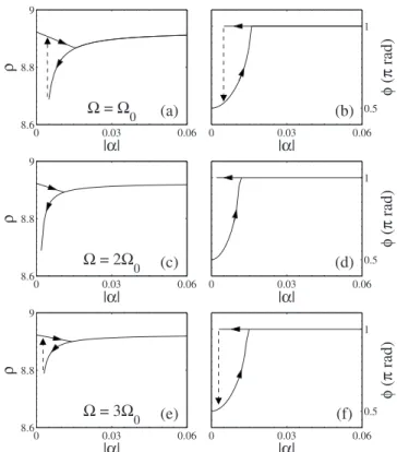
As mentioned, an imaginary amplitude of the modulation corresponds to the modulation of the cavity linear gain-loss parameters. Such modulation may involve different physical processes. Despite this difference, qualitatively, the action of gain-loss modulation can be similar to that of phase modulation. When the period of modulation is much smaller than the soliton separation, the action of linear gain-loss parameters tends to be averaged across the soliton pair. In that case, the periodic modulation can be approximated by constant parameters and the equa-tion is reduced to a pure CGLE. We consider here only two examples where such averaging does not happen completely. Namely, we choose ⍀=2⍀0 and ⍀=3⍀0. For
these two cases, we calculated both the soliton separation and the phase difference between the solitons as shown in Fig.5.
The diagrams for positive and negative ␣ are mirror images of each other due to the periodicity of the modula-tion. When increasing the amplitude of the modulation, we observe bifurcation and hysteresis phenomena that are very similar to those of Fig.2. Such similarity occurs in each case except for the specific values of␣ where the bifurcation occurs. Changes in soliton separation here are relatively small—much less than 1% of the total
separa-tion. At the same time, the phase difference between the solitons changes from/2 to . Thus, the phase difference is the main parameter to monitor in the experiments when observing this type of bifurcation. By comparing Figs.2and5, we can also conclude that soliton pairs are more robust against changes in the gain-loss parameters than in the case of phase modulation.
B. Medium Periods of Modulation
When ⍀ is comparable to ⍀0, we should expect
synchro-nization of the pulse separation with the modulation pe-riod. Figure6shows that indeed the soliton separation re-duces to the same value of the modulation period as the modulation amplitude兩␣兩 is increased. The soliton sepa-ration reduces from the original value 8.923 as兩␣兩 is in-creased until it approaches 7.19. We recall that positive and negative ␣ only shift the phase of the modulation. The phase difference between the solitons, being /2 at zero amplitude, sharply approaches zero at very small兩␣兩 and remains equal to zero upon further increases in the modulation amplitude. This happens as the soliton pair loses the ability to move freely at relatively small ampli-tudes of modulation and has to adjust the phase differ-ence to zero to stop transverse motion completely.
The synchronization itself can be seen in Fig. 7. Two solitons are compressed and their maxima coincide with the maxima of the periodic modulation. Further increases in the modulation depth兩␣兩 result in the generation of a pulse train in the crests of the periodic gain-loss modula-tion instead: this happens at around 兩␣兩=0.51 for ⍀ = 1.25⍀0.
For smaller modulation frequencies we can still observe similar synchronization. Namely, in Fig.8 the crosses on the vertical axes where兩␣兩=0 represent unperturbed soli-ton separation and phase difference. However, very small modulation兩␣兩⬍0.005 shifts these parameters to new val-ues ⬇2/⍀=11.153 and⬇ ± that correspond to the two solitons being attached to the maxima of the modula-tion pattern the same way as in Fig.7. Further increase in modulation amplitude hardly changes the new separa-tion and phase difference until the bifurcasepara-tion threshold is reached. The second transition appears when 兩␣兩 is around 0.24. It causes the single branch of soliton pair so-lutions to split into two new branches. One of the branches does not experience much change in the pair separation after the bifurcation, whereas the second branch appears with both a smaller pair separation and smaller phase difference. In each case after the
bifurca-0 0.1 0.2 6 8 10 |α| ρ
Fig. 4. Soliton pair separationversus the modulation depth␣ for the three cases shown in Fig.3. Namely,⍀=0.125⍀0(dashed curve),⍀=0.25⍀0 (dotted curve), and ⍀=0.5⍀0 (dashed-dotted
curve). 0 0.2 0.4 0.6 8.90 8.92 |α| ρ 0 0.2 0.4 0.6 0.5 1 |α| φ (π rad) 0 0.2 0.4 0.6 8.80 8.90 |α| ρ 0 0.2 0.4 0.6 0.5 1 |α| φ (π rad) (a) (b) Ω = 2Ω0 Ω = 3Ω0 (c) (d)
Fig. 5. [(a),(c)] Soliton pair separationand [(b),(d)] phase dif-ference between the pairversus the modulation depth兩␣兩 for modulation frequencies⍀=2⍀0and⍀=3⍀0, respectively.
0 0.2 0.4 0.6 7 8 9 |α| ρ Ω = (5/4)Ω0
Fig. 6. Soliton separationversus兩␣兩 for ⍀=1.25⍀0. Phase
dif-ference is zero in the whole interval except for a region of small 兩␣兩, which cannot be resolved in the scale of this figure.
tion, the position of the pair no longer remains at the maxima of the periodic modulation but shifts to its slopes. The pairs find new “equilibrium” positions in the periodic pattern, which are shown in Fig.9. The new equilibrium positions can be either on the same slope or on two differ-ent slopes. Each of these solutions may exist indepen-dently and they can also exist simultaneously, thus, cre-ating a bifurcation structure. When they are on the same slope, the pair separation remains at 11.153 and this cor-responds to the upper branch in Fig.8(a), while the lower branch represents the pair on two different slopes. At larger values of the modulation amplitude共兩␣兩⬎0.37兲, the instability of the zero amplitude background causes a train of pulses to be generated.
For each case shown in Figs. 6 and 8, there is also a region of bistability at very small兩␣兩 共⬍0.002兲, which is similar to those shown in Fig.6of [20]. The bifurcations and the corresponding hysteresis loops are too small to be seen in the scale of Figs.6and8. However, when⍀=⍀0,
this bistability disappears. The curves for soliton separa-tion and the phase difference shown in Fig. 10 are single valued. Upon varying兩␣兩, the pair separation and the phase difference change only slightly from their
ini-tial values. This shows that the influence of the periodic modulation in this case is minimal as should be expected. C. Large Periods of Modulation
As the imaginary amplitude of modulation␣ means that the gain-loss balance is modulated along the t axis, it rep-resents an addition to the linear loss term i␦ and can shift an area of original loss into gain. Thus, with the ap-plied periodic term, the conditions for generating solitons are changing with t. Solitons may become unstable at cer-tain points in time across the modulation period and some preferable positions for solitons along the t axis may be created. We can call them “equilibrium positions.” The latter are defined either by the overall balance between gain and loss or by the gradient of gain-loss across the pe-riod.
The equilibrium positions can be identified in numeri-cal simulations just by propagating solitons. Whichever positions they had initially, single solitons or pairs of them will eventually move to the equilibrium position. For the chosen values of the system parameters, the
equi-−15 0 15 0 1 2 t |ψ | α = −0.4i
Fig. 7. Location of two solitons (solid curve) in the pair relative to the pattern of periodic gain-loss modulation (dashed curve) for ⍀=1.25⍀0and␣= −0.4i. 0 0.2 0.4 8 10 12 |α| ρ 0 0.2 0.4 0 0.5 1 |α| φ (π ra d ) Ω = (4/5)Ω0 (a) (b)
Fig. 8. Soliton separationand phase difference between the solitons versus兩␣兩 for ⍀=0.8⍀0. The crosses on the vertical axes where兩␣兩=0 represent unperturbed soliton separation and phase difference. Very small modulation兩␣兩⬍0.002 shifts these param-eters to new values⬇11.153 and= that stay almost fixed until the bifurcation threshold is reached. Splitting into two types of solitons occurs at 兩␣兩⬇0.24. Soliton pairs above this threshold have branches of 0,/ 2, and phase difference be-tween the pulses. The arrows show the sequence of changes when increasing or decreasing兩␣兩.
−15 0 15 0 1 2 t |ψ | −15 0 15 0 1 2 t |ψ | (a) (b)
Fig. 9. Location of two solitons (solid curve) in the pair relative to the pattern of periodic modulation (dashed curve) for ⍀ = 0.8⍀0and ␣= −0.3i. Solitons prefer certain equilibrium
posi-tions in the pattern thus comprising two types of bound states. (a) The solution representing the upper branch and (b) the lower branch in Fig.8(a).
0 0.1 0.2 0.3 8.85 8.90 8.95 |α| ρ 0 0.1 0.2 0.3 0.4 0.6 0.8 |α| φ (π rad) (a) (b) Ω = Ω0
Fig. 10. (a) Soliton pair separationand (b) the phase differ-ence versus the gain-loss modulation depth兩␣兩 for period of modulation⍀=⍀0.
librium positions of solitons found in that way are shown in Figs. 11 and 12. Clearly, these equilibrium positions vary with the amplitude of modulation␣. The cases of two smaller ␣ are presented in Fig. 11 while the case of ␣ = 0.3i is shown separately in Fig.12.
When the amplitude of the modulation is␣=0.1i, which is smaller than the linear loss term␦= 0.2, the modulation does not destroy the soliton pair. Starting from any point within the period of the modulation, the pair moves to one of the equilibrium positions shown in Fig.11(a). It may be located either on the negative or positive slope of the po-tential. Only one of them is shown in the plot.
An example of soliton pair evolution in this case is shown in Fig.13(a). In this example, the pair is initially located at t = 0 where the linear loss is minimal. The pair moves to the right because of the specified positive sign of the phase difference/2 between the solitons in the pair. If the sign is negative, the pair moves to the left. In a short distance, the pair arrives to the equilibrium position and stays there forever. In this simulation, the pair con-tinues to oscillate around the equilibrium state approach-ing the limit cycle. For other sets of parameters, the limit cycle may be transformed into a fixed point.
For higher value of the amplitude␣=0.2i, the gain is exactly balanced with loss at t = 0. At other values of t the linear loss prevails. The bound state does not exist and the pair splits into two separate solitons. Two equilibrium states of solitons for this case are shown in Fig. 11(b). They are located symmetrically on the positive and
nega-tive slopes of the gain-loss curve. As the background for the dissipative terms stays negative, noise does not grow and single solitons are stable across the whole periodic potential. Equilibrium positions are shifted closer to the center t = 0 in comparison with the case with␣=0.1i. The soliton pair becomes unstable and splits into two indepen-dent solitons right from the beginning of its evolution. The simulation showing this behavior is displayed in Fig. 13(b). After splitting, each soliton moves to the equilib-rium position being fixed for the rest of the simulation.
An interesting case occurs when the modulation ampli-tude␣=0.3i. As this value is higher than the linear loss term␦= 0.2, there are two points at the modulation curve that cancel gain loss in the linear approximation. These are approximately the equilibrium states of the solitons. They are shown in Fig.12. The interval between the equi-librium positions is unstable as the linear gain is positive here. Thus, additional solitons may be created due to the spontaneous amplification of noise. One of them is shown in Fig.12. The simulation starting from the soliton pair shows its splitting (see Fig. 13) and the moving of each soliton to its equilibrium position. A third soliton is cre-ated between them. It moves chaotically due to the insta-bility of the background. At some z, two solitons may exist simultaneously in the region of instability.
5. CONCLUSIONS
We studied the dynamics of bound solitons of the complex cubic-quintic Ginzburg–Landau equation (CGLE) under
−300 −15 0 15 30 1 2 t |ψ | (a) α = 0.1i −300 −15 0 15 30 1 2 t |ψ | (b) α = 0.2i
Fig. 11. Equilibrium positions of the soliton pairs and single solitons shown by solid curves when (a)␣= 0.1i and (b)␣= 0.2i. Dashed curve shows the periodic linear gain-loss function with ⍀=0.125⍀0. −300 −15 0 15 30 1 2 t |ψ | α = 0.3i
Fig. 12. Equilibrium state of single solitons when␣= 0.3i. An additional soliton appears in the middle due to the instability of the background. Its position is not fixed and may vary along t in evolution. Dashed curve shows the periodic linear gain-loss func-tion with⍀=0.125⍀0. −20 0 20 0 1 2 t z |ψ| (a) 0 25000 50000 −20 0 20 0 1 2 t z |ψ| (b) 0 25000 50000 −20 0 20 0 1 2 t z |ψ| (c) 0 25000 50000
Fig. 13. Soliton pair evolution under the effect of the gain-loss modulation with⍀=0.125⍀0(dashed line). (a)␣= 0.1i; the pair
remains bounded and occupies the equilibrium position as a bound state. (b)␣= 0.2i; the pair splits and each soliton occupies the equilibrium position. (c)␣= 0.3i; the pair splits and each soli-ton occupies the equilibrium position in the periodic potential well. The background between the two solitons is unstable creat-ing additional chaotically movcreat-ing solitons.
the influence of external phase and gain-loss modulation. We considered periods of modulation being larger or smaller than the soliton separation and the amplitude of modulation being either real or imaginary. In the former case the modulation influences the soliton separation while in the latter case solitons split and end up finding a position in the two equilibrium states of the periodic po-tential. We illustrated the complicated dynamics of this process by a few numerical examples. These results may become useful in experimental studies of lasers that have simultaneously passive and active mode-locking mecha-nisms. One of the possibilities found in this work has been confirmed in the experimental results of [19]. Other cases considered here are also worthy of experimental observa-tion.
ACKNOWLEDGMENT
N. Akhmediev and W. Chang gratefully acknowledge the support of the Australian Research Council (Discovery project DP0985394).
REFERENCES
1. A. J. DeMaria, D. A. Stetser, and H. Heynau, “Self mode locking of lasers with saturable absorbers,” Appl. Phys. Lett. 8, 174–176 (1966).
2. K. Sala, M. C. Richardson, and N. R. Isenor, “Passive mode locking of lasers with the optical Kerr effect modulator,” IEEE J. Quantum Electron. 13, 915–924 (1977).
3. F. Krausz and T. Brabec, “Passive mode locking in standing-wave laser resonators,” Opt. Lett. 18, 888–890 (1993).
4. E. P. Ippen, “Principles of passive mode locking,” Appl. Phys. B 58, 159–170 (1994).
5. O. E. Martinez, R. L. Fork, and J. P. Gordon, “Theory of passively mode-locked lasers including self-phase modulation and group-velocity dispersion,” Opt. Lett. 9, 156–158 (1984).
6. F. X. Kärtner and U. Keller, “Stabilization of solitonlike pulses with a slow saturable absorber,” Opt. Lett. 20, 16–18 (1995).
7. R. Paschotta and U. Keller, “Passive mode locking with slow saturable absorbers,” Appl. Phys. B 73, 653–662 (2001).
8. G. Palmer, M. Emons, M. Siegel, A. Steinmann, M. Schultze, M. Lederer, and U. Morgner, “Passively mode-locked and cavity-dumped Yb:KY(WO4)2 oscillator with positive dispersion,” Opt. Express 15, 16017–16021 (2007). 9. N. Akhmediev, J. M. Soto-Crespo, and G. Town, “Pulsating solitons, chaotic solitons, period doubling, and pulse coexistence in mode-locked lasers: CGLE approach,” Phys. Rev. E 63, 056602 (2001).
10. N. Akhmediev and A. Ankiewicz, Dissipative Solitons (Springer, 2005).
11. S. Wabnitz, “Suppression of soliton interaction by phase modulation,” Electron. Lett. 29, 1711–1712 (1993). 12. L. E. Hargrove, R. L. Fork, and M. A. Pollack, “Locking of
He-Ne laser modes induced by synchronous intracavity modulation,” Appl. Phys. Lett. 5, 4–5 (1964).
13. G. R. Huggett, “Mode locking of CW lasers by regenerative RF feedback,” Appl. Phys. Lett. 13, 186–187 (1968). 14. H. A. Haus, “A theory of forced mode locking,” IEEE J.
Quantum Electron. 11, 323–330 (1975).
15. J. N. Kutz, B. C. Collings, K. Bergman, S. Tsuda, S. T. Cundiff, and W. H. Knox, “Mode-locking pulse dynamics in a fiber laser with a saturable Bragg reflector,” J. Opt. Soc. Am. B 14, 2681–2690 (1997).
16. J. D. Moores, “Oscillating solitons in a novel integrable
model of asynchronous mode locking,” Opt. Lett. 26, 87–89 (2001).
17. J. J. O’Neil, J. N. Kutz, and B. Sandstede, “Theory and simulation of the dynamics and stability of actively mode-locked lasers,” IEEE J. Quantum Electron. 38, 1412–1418 (2002).
18. N. D. Nguyen and L. N. Binh, “Generation of bound solitons in actively phase modulation mode-locked fiber ring resonators,” Opt. Commun. 281, 2012–2022 (2008). 19. W.-W. Hsiang, C.-Y. Lin, and Y. Lai, “Stable new bound
soliton pairs in a 10 GHz hybrid frequency modulation mode-locked Er-fiber laser,” Opt. Lett. 31, 1627–1629 (2006).
20. W. Chang, N. Akhmediev, and S. Wabnitz, “Effect of external periodic potential on pairs of dissipative solitons,” Phys. Rev. A 80, 013815 (2009).
21. W.-W. Hsiang, C.-Y. Lin, M.-F. Tien, and Y. Lai, “Direct generation of a 10 GHz 816 fs pulse train from an erbium-fiber soliton laser with asynchronous phase modulation,” Opt. Lett. 30, 2493–2495 (2005).
22. I. Aranson and L. Kramer, “The world of the complex Ginzburg–Landau equation,” Rev. Mod. Phys. 74, 99–143 (2002).
23. H. A. Haus, “Theory of mode locking with a slow saturable absorber,” IEEE J. Quantum Electron. 11, 736–746 (1975). 24. H. A. Haus, “Theory of mode locking with a fast saturable
absorber,” J. Appl. Phys. 46, 3049–3058 (1975).
25. A. Komarov, H. Leblond, and F. Sanchez, “Quintic complex Ginzburg–Landau model for ring fiber lasers,” Phys. Rev. E
72, 025604(R) (2005).
26. W. H. Renninger, A. Chong, and F. W. Wise, “Dissipative solitons in normal-dispersion fiber lasers,” Phys. Rev. A 77, 023814 (2008).
27. J. D. Moores, “On the Ginzburg–Landau laser mode-locking model with fifth-order saturable absorber term,” Opt. Commun. 96, 65–70 (1993).
28. S. T. Cundiff, J. M. Soto-Crespo, and N. Akhmediev, “Experimental evidence for soliton explosions,” Phys. Rev. Lett. 88, 073903 (2002).
29. J. M. Soto-Crespo, N. Akhmediev, Ph. Grelu, and F. Belhache, “Quantized separations of phase-locked soliton pairs in fiber lasers,” Opt. Lett. 28, 1757–1759 (2003). 30. J. M. Soto-Crespo, M. Grapinet, Ph. Grelu, and N.
Akhmediev, “Bifurcations and multiple period soliton pulsations in a passively mode-locked fiber laser,” Phys. Rev. E 70, 066612 (2004).
31. J. M. Soto-Crespo, Ph. Grelu, N. Akhmediev, and N. Devine, “Soliton complexes in dissipative systems: vibrating, shaking, and mixed soliton pairs,” Phys. Rev. E
75, 016613 (2007).
32. H. R. Brand and R. J. Deissler, “Interaction of localized solution for subcritical bifurcations,” Phys. Rev. Lett. 63, 2801–2804 (1989).
33. B. A. Malomed, “Bound solitons in the nonlinear Schrodinger–Ginzburg–Landau equation,” Phys. Rev. A 44, 6954–6957 (1991).
34. N. N. Akhmediev, A. Ankiewicz, and J. M. Soto-Crespo, “Stable soliton pairs in optical transmission lines and fiber lasers,” J. Opt. Soc. Am. B 15, 515–523 (1998).
35. D. Turaev, S. Zelik, and A. Vladimirov, “Chaotic bound states of localized structures in the complex Ginzburg–Landau equation,” Phys. Rev. E 75, 045601 (2007).
36. N. Akhmediev, A. Ankiewicz, and J. M. Soto-Crespo, “Multisoliton solutions of the complex Ginzburg–Landau equation,” Phys. Rev. Lett. 79, 4047–4051 (1997).
37. Ph. Grelu and N. Akhmediev, “Group interactions of dissipative solitons in a laser cavity: the case of 2 + 1,” Opt. Express 12, 3184–3189 (2004).
38. Ph. Grelu, F. Belhache, F. Gutty, and J. M. Soto-Crespo, “Phase-locked soliton pairs in a stretched-pulse fiber laser,” Opt. Lett. 27, 966–968 (2002).
39. Ph. Grelu, F. Belhache, F. Gutty, and J. M. Soto-Crespo, “Relative phase locking of pulses in a passively mode-locked fiber laser,” J. Opt. Soc. Am. B 20, 863–870 (2003).

![Fig. 5. [(a),(c)] Soliton pair separation and [(b),(d)] phase dif- dif-ference between the pair versus the modulation depth 兩 ␣ 兩 for modulation frequencies ⍀=2⍀ 0 and ⍀=3⍀ 0 , respectively.](https://thumb-eu.123doks.com/thumbv2/123dokorg/5527637.64693/4.918.81.443.807.1057/soliton-separation-ference-versus-modulation-modulation-frequencies-respectively.webp)


