A macroeconomic evaluation of energy efficiency objectives using GDyn-E ita model

(1)

A MACROECONOMIC EVALUATION OF ENERGY

EFFICIENCY OBJECTIVES USING GDyn-E ITA MODEL

CHIARA MARTINI

ENEA - Dipartimento Unità Efficienza Energetica Monitoraggio e Supporto alle Politiche di Efficienza Energetica

Sede Legale, Roma

(2)

AGENZIA NAZIONALE PER LE NUOVE TECNOLOGIE, L’ENERGIA E LO SVILUPPO ECONOMICO SOSTENIBILE

A MACROECONOMIC EVALUATION OF ENERGY

EFFICIENCY OBJECTIVES USING GDyn-E ITA MODEL

CHIARA MARTINI

ENEA - Dipartimento Unità Efficienza Energetica Monitoraggio e Supporto alle Politiche di Efficienza Energetica

Sede Legale, Roma

(3)

I contenuti tecnico-scientifici dei rapporti tecnici dell'ENEA rispecchiano l'opinione degli autori e non necessariamente quella dell'Agenzia.

The technical and scientific contents of these reports express the opinion of the authors but not necessarily the opinion of ENEA.

I Rapporti tecnici sono scaricabili in formato pdf dal sito web ENEA alla pagina http://www.enea.it/it/produzione-scientifica/rapporti-tecnici

(4)

A MACROECONOMIC EVALUATION OF ENERGY EFFICIENCY OBJECTIVES USING GDyn-E ITA MODEL

CHIARA MARTINI

Riassunto

In questo lavoro sono valutati gli impatti macroeconomici degli obiettivi indicativi nazionali di efficienza energetica al 2020 e dell’obiettivo Europeo al 2030. In particolare, l’analisi è focalizzata su tre paesi dell’EU15, rappresentati da Italia, Germania e Spagna, dove è simulata anche l’introduzione di un fondo nazionale per l’efficienza energetica. Il modello di equilibrio economico generale GTAP è utilizzato nella sua versione dinamica energetica, denominata GDyn-E. Questo modello consente di calcolare gli impatti su variabili macroeconomiche chiave, come PIL, valore aggiunto settoriale e totale, commercio internazionale, occupazione.

Le variabili considerate da GDyn-E sono analoghe a quelle incluse nelle Valutazioni di Impatto della Commissione Europea. Il modello GDyn-E può essere usato in futuro per fornire ulteriori stime degli impatti delle politiche energetiche Europee in Italia e altri paesi membri. Le stime elaborate potranno essere affiancate a quelle esistenti così da ampliare il range degli impatti di medio lungo termine sottoposti a valutazione.

Parole chiave: Equilibrio Economico Generale, GTAP, efficienza energetica, impatti macroeconomici

Abstract

The macroeconomic impacts of the 2020 energy efficiency national indicative targets, as well as those of the more recent EU 2030 objective, are assessed in this work. In particular, the analysis is focused on three EU15 countries, namely Italy, Germany and Spain, in which the introduction of national fund for energy efficiency is simulated.

The GTAP Computable General Equilibrium model is used, in its dynamic energy version GDyn-E. This model allows to compute the impacts on key macroeconomic variables, such as GDP, total and sectoral value added, international trade, and employment.

The variables considered by GDyn-E are analogous to those included in the Impact Assessment documents elaborated by the European Commission. GDyn-E model could be used in the future to provide further estimates of EU energy policy impacts in Italy and other member countries. These estimates could be put together with the existing ones in order to enlarge the range of medium-term impacts available in policy evaluation.

(5)

(6)

1 Introduction

The present work is aimed to study the macroeconomic impacts of medium-term EU energy efficiency policies, introducing 2020 and 2030 objectives. The Directive 27/2012 (Energy Efficiency Directive, EED) introduces national indicative targets for 2020, while the 2030 Energy Strategy, as defined by the EU Communication published in October 2014 (COM(2014) 15 final), sets an EU-wide non-binding energy efficiency target. In particular, the analysis will be focused on three EU15 countries, namely Italy, Germany and Spain, and both the country-specific EED objectives and the EU-wide energy efficiency goal will be introduced.

The evaluation of the macroeconomic impacts of energy policies - such as those introduced with the above mentioned EU legislation and communication - should take into account the international trade dimension. Thus, global modelling tools are needed, in order to assess the changes in trade competitiveness. In this work, GTAP Computable General Equilibrium (CGE) model has been used, in its dynamic energy version GDyn-E (Antimiani et al., 2013), allowing to explicitly modelling energy sectors and the corresponding commodities. GDyn-E in fact is characterised by a production function with substitutability among intermediate energy inputs (oil, coal, gas, oil

products and electricity). The computation of CO2 emissions is based on energy used by final use

sectors.

GDyn-E allows to compute the impacts on key macroeconomic variables, such as GDP, total and sectoral value added, international trade, and employment. It also provides information on energy commodities demand and the cost of emission reduction in terms of carbon tax. The model can be used to perform long term environmental-energy policy assessment, investigating how changes in policy, technology, and primary factor endowments affect the path of economies over time.

This work aims to show how the variables considered by a macroeconomic model such as GDyn-E are analogous to those included in the Impact Assessment documents elaborated by the European Commission (Directive 27/2012 Impact Assessment, SEC(2011) 779 final; Communication

(2014)15 Impact Assessment, SWD(2014) 255 final)1. For this exercise, the EED objectives for

2020, as well as the EU 2030 objective set in the Commission Communication (2014)15 and then in

1_{In the following sections, the comparison with the results included in the mentioned Impact Assessments will not be}

performed, since in Directive 27/2012 Impact Assessment a completely different type of model is used (E3ME), while the construction of scenario could not be harmonised with the Communication (2014)15 Impact Assessment, in particular relative to the information used to build up the baseline and the level of detail in energy policies modelisation. Another difference is given by the fact that the general equilibrium model GEM-E3 employed in the Communication (2014)15 Impact Assessment treats differently the labour market.

(9)

8

October Communication of the European Council (EUCO 169/14), have been introduced in the GDyn-E model.

2 The GDyn-E model

GTAP is a CGE model developed in the framework of the Global Trade Analysis Project (GTAP; Hertel 1997), coordinated by the Purdue University, Indiana. The GTAP consortium elaborates and periodically revises also the GTAP Database, including of 134 regions defined as aggregates of 244 countries or regions, as described in the GTAP standard country list. As for sectoral disaggregation, 57 sectors are considered (Narayan et al., 2012).

Different versions of the GTAP model exist, among which GDyn-E (Golub, 2013) features in detail

the structure of energy consumption, both in industrial and residential sectors, and includes CO2

emissions and the possibility to simulate carbon taxation and emission trading. The GDyn-E model is obtained by merging the dynamic version of GTAP (Ianchovichina, E.,McDougall 2001) with the last version of static GTAP-Energy model (Burniaux and Truong, 2002). GDyn-E model is

originally based on version 7 of GTAP Data Base2.

This work is based on an improved version of GDyn-E model (Antimiani et al. 2013), developed jointly by ENEA (Energy Efficiency Unit and Studies and Strategies Unit), the Department of

Economics of Roma III University and the National Institute of Agricultural Economics (INEA)3.

Relatively to the standard GDyn-E database and model, several changes have been introduced, for example with respect to the sectoral substitution elasticities in the different energy nests,

technological progress variables, equity market representation and procedure for calibrating CO2

emissions. The model has been extensively used for evaluations in different public policies domains, for example relative to the impacts of unilateral decarbonisation policies on international competitiveness (Antimiani et al., 2013), different options for taxing emission trading permits (Costantini et al., 2013), and different negotiating and financing options in global climate agreements (Markandya et al., 2015). This improved version of GDyn-E model is based on version

8 of GTAP Data Base4.

A CGE model such as GDyn-E offers a top-down representation of the national economic system and thus it is suited for economy-wide analyses of the implications of energy and emission policies.

2 _For _more _detail, _see _GTAP ₇ _Data _Base _{Documentation,} _available _here https://www.gtap.agecon.purdue.edu/databases/v7/v7_doco.asp

3

INEA has recently changed its name and organisation in Council for Agricultural Research and Economics (CREA). 4 _For _more _detail, _see _GTAP ₈ _Data _Base _{Documentation,} _available _here https://www.gtap.agecon.purdue.edu/databases/v8/v8_doco.asp

(10)

9

By contrast, due to the way economic relationships are modelled and the kind of included data, GDyn-E cannot provide a technology-rich representation of the different options available for

energy efficiency and CO2 emission reduction. To overcome this limitation, a soft-linkage between

GDyn-E and the bottom-up model Times-Italy has been recently developed, in the framework of the Deep Decarbonisation Pathways Project (Virdis et al., 2015). In this exercise, the decarbonisation objectives implemented in Times-Italy have been feeded in GDyn-E and also in ICES, another CGE model used by the Fondazione Eni Enrico Mattei (FEEM), in terms of primary and final energy mix, so that their macroeconomic implications could be analysed.

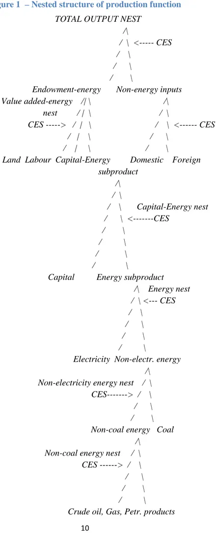
The production functions are specified via a series of nested Constant Elasticity of Substitution (CES) functions (Figure 1). Sectoral output is a function of technology, aggregate value added-energy composite, and other intermediate inputs. Value added is produced using primary factors, namely land, labour, natural resources, and a energy composite. At its turn, the capital-energy composite is produced by combining capital and capital-energy, having a limited possibility to substitute energy for capital (Golub, 2013; Antimiani et al., 2013). In a lower nest, electricity can be substituted with electrical energy, while in the next lower nest coal can be substituted with non-coal energy sources. The lowest layer of nesting accounts for the choice among the remaining energy commodities, namely oil, gas, and oil products. Non-fossil energy sources – nuclear and renewable energy – are not represented in the model. Each production sector has specific substitution possibilities which are an indirect representation of the main existing and adopted technologies. In particular, substitution possibilities also proxy the use of renewable energy, which is not explicitly included in GDyn-E model, as will be further explained in the following.

Goods imported from different countries are not perfect substitutes, and the substitution possibilities are modelled according to the so-called “Armington” assumption. According to it, in GDyn-E model smaller and more realistic responses to price changes are generated relative to the responses observed in models of homogeneous imported products. When their price changes, imported goods could be substituted with the same goods coming from other countries, according to the values of Armington elasticities. Of course, in the model imported goods are chosen basing on the production costs and on relative prices in different countries.

The model uses physical emission coefficients for each fossil fuel (coal, oil, gas and oil products) which are constant across sectors and regions of the world economy (Truong and Lee, 2003). Only

CO2 emissions from energy use in the industrial processes and final household consumption are

(11)

10

Figure 1 – Nested structure of production function

TOTAL OUTPUT NEST /\

/ \ <--- CES / \

/ \ / \

Endowment-energy Non-energy inputs Value added-energy /| \ /\ nest / | \ / \

CES ---> / | \ / \ <--- CES / | \ / \

/ | \ / \

Land Labour Capital-Energy Domestic Foreign subproduct /\ / \ / \ Capital-Energy nest / \ <---CES / \ / \ / \ / \

Capital Energy subproduct

/\ Energy nest / \ <--- CES / \ / \ / \ / \

Electricity Non-electr. energy /\

Non-electricity energy nest / \ CES---> / \ / \ / \ Non-coal energy Coal

/\ Non-coal energy nest / \ CES ---> / \ / \ / \ / \

(12)

11

With the simulation of baseline and policy scenarios, the GDyn-E model enables to assess the time impacts of energy policies on macroeconomic variables, such as

• Gross Domestic Product (GDP)

• Sectoral output and value added

• Sectoral import and export

• Net trade balance

• Sectoral employment and its distribution between skilled and unskilled labour force

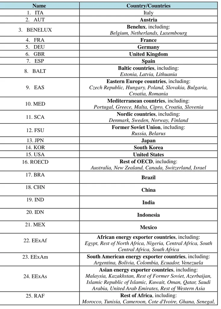
The total number of countries and sectors included in the model can be customised according to the specific features of the analysed problem. In the current analysis, a relatively high disaggregation level has been chosen for the European Union countries, since specific energy efficiency objectives were simulated. In particular, all major European economies have been disaggregated, and the other EU members have been aggregated in regional groups (Table 1). The version of GDyn-E just described is called GDyn-E ITA.

(13)

12

Table 1 – Countries included in GDyn-E ITA

Name Country/Countries

1. ITA Italy

2. AUT Austria

3. BENELUX Benelux, including:

Belgium, Netherlands, Luxembourg

4. FRA France

5. DEU Germany

6. GBR United Kingdom

7. ESP Spain

8. BALT Baltic countries, including:

Estonia, Latvia, Lithuania

9. EAS

Eastern Europe countries, including:

Czech Republic, Hungary, Poland, Slovakia, Bulgaria, Croatia, Romania

10.MED Mediterranean countries, including:

Portugal, Greece, Malta, Cipro, Croatia, Slovenia

11.SCA Nordic countries, including:

Denmark, Sweden, Norway, Finland

12.FSU Former Soviet Union, including:

Russia, Belarus

13.JPN Japan

14.KOR South Korea

15. USA United States

16. ROECD Rest of OECD, including:

Australia, New Zealand, Canada, Switzerland, Israel 17. BRA Brazil 18. CHN China 19. IND India 20. IDN Indonesia 21. MEX Mexico

22. EExAf African energy exporter countries, including:

Egypt, Rest of North Africa, Nigeria, Central Africa, South Central Africa, South Africa

23. EExAm South American energy exporter countries, including:

Argentina, Bolivia, Colombia, Ecuador, Venezuela

24. EExAs

Asian energy exporter countries, including: Malaysia, Kazakhstan, Rest of Former Soviet, Azerbaijan,

Islamic Republic of Islamic, Kuwait, Oman, Qatar, Saudi Arabia, United Arab Emirates, Rest of Western Asia

25. RAF Rest of Africa, including:

(14)

13

Rest of Western Africa, Ethiopia, Kenya, Rwanda, Togo, Guinea, Benin, Burkina Faso, Madagascar, Malawi, Mauritius, Mozambique, Tanzania, Uganda, Zambia, Zimbabwe, Rest of Eastern Africa, Botswana, Namibia, Rest of

South African

26. RAM

Rest of America, including:

Rest of North America, Chile, Paraguay, Peru, Uruguay, Rest of South America, Costa Rica, Guatemala, Honduras, Nicaragua, Panama, El Salvador, Rest of Central America,

Caribbean

27. RAS

Rest of Asia, including:

Rest of Oceania, Mongolia, Taiwan, Rest of East Asia, Cambodia, Lao People's Democratic Republic, Philippines,

Singapore, Thailand, Viet Nam , Rest of Southeast Asia, Bangladesh, Nepal, Pakistan, Sri Lanka, Rest of South Asia,

Kyrgyztan, Armenia, Bharain

28. REU Rest of Europe, including:

Rest of EFTA, Albania, Ukraine, Rest of Eastern Europe, Rest of Europe, Georgia, Turkey, Rest of the world

(15)

14

At sectoral level, energy intensive sectors have been detailed in the model, in order to be able to provide a better assessment of the impacts associated to energy efficiency policies (Table 2).

Table 2 – Sectors included in GDyn-E ITA

Name Sector/sectors

1. AGR Agriculture, including:

Paddy rice; Wheat; Cereal grains nec; Vegetables, fruit, nuts

Oil seeds; Sugar cane, sugar beet; Plant-based fibers

Crops nec; Bovine cattle, sheep and goats, horses; Animal products nec; Raw milk; Wool, silk-worm

cocoons; fishing; forestry.

2. COAL Coal

3. GAS Natural gas

4. OIL Oil

5. OIL_PCTS Refinery

6. ELECTRICITY Electricity

7. IRON_STEEL Iron and steel

8. CHEM_PETROC Chemical and petrolchemical

9. NON_FERMETAL Non-ferrous metals

10.NON_METMIN Non-metallic minerals

11.TRANSEQP Transport equipment, including:

Metal products; Motor vehicles and parts; Other transport equipment

12.MACHINERY Electronic and machinery equipment

13.OTH_MANUF Other manufacturing

14.FOOD_TOB Food and tobacco, including:

Bovine cattle, sheep and goat meat products; Meat products; Vegetable oils and fats; Dairy products; Processed rice; Sugar; Beverages and

tobacco products

15.PAPER Paper

16.WOOD Wood products

17.CONSTRUCT Construction

18.TEXTILE Textile, including:

Textiles; Wearing apparel; Leather products

19.LAND_TRASP Road transport

20.AIR_TRANS Air transport

21.WATER_TRANS Water transport

22.SERVICES Services, including:

Water; Trade; Communication; Financial services nec; Insurance; Business services nec; Recreational

and other services; Public Administration, Defense, Education, Health; Dwellings

(16)

15

The model analyses the temporal horizon 2007-2030, in five intervals (2007-10; 2010-15; 2015-20; 2020-25;2025-30). The base year is 2007.

3 Simulations

In the following, the construction of both baseline and policy scenarios will be outlined. It is worth mentioning once again that the final aim of this work is not providing accurate policy scenario estimates, which as in every modelling exercise depend on the assumptions and mirror only one among the different possible evolution of the system. The main purpose is instead showing the potential of a macroeconomic model such as GDyn-E, in terms of information it is able to provide, and pointing out how this information can be compared with existing one, for example from the EU Impact Assessments, in terms of differences from the baseline.

Three scenarios have been elaborated, basing on the same macroeconomic baseline assumptions on population, skilled and unskilled labour force. The information about the long term evolution of such variables has been taken from World Bank and International Labour Organisation (ILO). GDP evolution is exogenously given to the model in the baseline scenario, using World Bank projections, whereas it is endogenously computed in the two policy scenarios, as deviation from the baseline trends.

The first scenario is represented by the baseline, in which emissions have been assumed to follow an increasing trend, comparable with available projections (European Commission, 2008) for EU countries and consistent to the Current Policies scenario in the World Energy Outlook 2013 (WEO, 2013) for extra-EU countries.

Additionally, the two policy scenarios hypothesize that EU28 countries reduce their energy consumption – and thus their emissions – according to the EED and October Communication objectives. As for extra-EU countries, no energy policy has been introduced.

3.1 Baseline scenario

This paragraph will illustrate the trends of exogenous variables in the baseline (or reference) scenario.

Relatively to 2010, in 2030 population would grow by 8% in the EU and 26% in the whole world, in line with the projections provided by the World Bank. As for labour force, different trends are observed in the EU, with Italy and Spain showing smaller growth rates, which in Italy would be equal on average to 1.4% per year for skilled employees and to 1.1% for unskilled, over the period

(17)

16

2010-2030. Other countries, among which Germany, would show higher growth rates. These trends are provided by ILO. GDP is assumed to grow on average around 2% per year from 2010 to 2030. In Italy, GDP would have an average growth equal to 1.2% per year in the same period. It is important to be informed about the trends followed by these variables in the baseline scenario, in particular regarding to GDP, in order to be able to correctly interpret policy results as deviation from the baseline tendencies.

As for emissions, in the baseline they would not be limited by any reduction target, namely the scenario will model emissions growth as it would be without any policy intervention introducing sectoral or national constraints. This choice enables to isolate the effects associated to the 2020 energy efficiency policy objectives. Alternatively, EU and national policies could have been included in the baseline, and this would have lowered the macroeconomic impacts, which in this

exercise should be considered as being in the upper bound of available literature estimates5. In Italy,

emissions are assumed to increase on average by 0.7% per year over the period 2010-2030, while in Germany the growth rate is 0.3%.

To conclude this brief description of baseline scenario, it is worth mentioning the importance of the reference against which targets are set, both in modelling exercises and in real-world climate negotiations or energy efficiency policies elaboration. Indeed, when the 20% emission reduction objective was set, the 2020 baseline was provided the Primes 2007 scenario (European

Commission, 2008)6. In 2010, Italy emissions turned out to be already below the 2020 objective,

partly due to the effect of the economic crisis and partly to the first effects of the implemented energy policies. The same is true for other EU countries. In this simulation, reference emissions have been calibrated basing on historical values for 2010, and they have been assumed to have an

increasing trend in the following years7. The policy objective equal to a 20% reduction in 2020 was

then established relative to the 2020 baseline value, which shows a relative small difference from Primes 2007 scenario (European Commission, 2008) and a higher one from Primes 2013 scenario (European Commission, 2014). Relatively to the 2030 objective, equal for the EU to a 40%

5

This approach is consistent with the approach adopted in the Italian National Energy Strategy to build up the scenario “Assenza misure”.

6_{Primes is a partial equilibrium model, developed by the National Technical University of Athens, and adopted by the}

European Commission Impact Assessments of energy policy impacts.

7

It is worth mentioning that the ratio between emission and energy consumption levels is altered in GDyn-E by the absence of an explicit consideration of renewable energy. Thus, the emissions corresponding to the 2020 energy efficiency objectives are higher than in the real world, since in GDyn-E only fossil fuel energy is considered. Moreover, another reason why emissions levels are relatively high, for example if compared to Primes 2013 scenario, is that policies implemented up to 2013 are not included in the baseline, as explained before.

(18)

17

reduction relatively to 1990 emission level, it has been calculated that for the EU as whole this would also correspond to about a 30% reduction relative to 2030 baseline emission level.

Finally, energy consumption levels have been calibrated to historical values in 2010. Later on, an increasing trend has been assumed but at a slower rate than in Primes 2007 scenario, for individual countries and consequently for the EU as a whole. Consumption levels are more aligned with Primes 2013 scenario. For Italy, in particular, 2020 baseline primary and final consumption levels are aligned also with the National Energy Strategy (scenario “Assenza misure”).

3.2 Policy scenarios

This paragraph will describe the two implemented policy scenarios, providing details on the policy objectives and on the strategy adopted for modelling key issues such as energy efficiency and renewable energy.

Consistently with the 20-20-20 objectives set in the European 2020 Strategy (COM(2010) 2020),

the two policy scenarios envisage a 20% CO2 emission reduction at EU level in 2020, together with

a 20% reduction of primary energy consumption, in both cases relative to the baseline. As for

different EU member countries, the national indicative objectives introduced in the Directive

27/2012 are modelled, and emissions would change accordingly. In 2030, CO2 emission are reduced

by 40% relative to 1990 levels, as set by the 2030 Energy Strategy (COM(2014) 15 final). Energy efficiency plays a key role in achieving this objective, improving by 27% relative to the baseline. In member countries, emissions, primary and final energy consumption would change consistently with the EU-level 2030 objective to be reached.

As already explained, the final aim of the two policy scenarios is to show the potential of GDyn-E model in evaluating macroeconomic impacts of emission and energy efficiency objectives. The art. 20 of Directive 27/2012 introduces the possibility to set up national funds for energy efficiency, in order to support national energy efficiency initiatives and enhance the achievement of national objectives. According to the Directive, revenue from annual emission allocations in the EU Emission Trading Scheme (ETS) could be used to finance the fund. A simplified version of the National Fund for Energy Efficiency – as introduced in Italy with the Legislative Decree 102/2014 – is implemented in the second policy scenario (FUND scenario, in opposition to the NO FUND scenario). The Italian fund is designed to facilitate efforts for the rehabilitation of buildings of the public sector and the reduction of energy consumption in the sectors of industry and services, through the granting guarantees. According to the Decree, it should be fuelled with EUR 25 million in 2015, which could be increased to a more than double amount, reaching EUR 490 million for the

(19)

18

whole 2014-2020 period (2014 National Energy Efficiency Action Plan). The fund is not yet operational.

It is worth noticing that in Spain a national fund for energy efficiency has been constituted in 2015, with a yearly budget of EUR 350 million, to be financed by the central government (45%) and by power companies (55%) through an obligation scheme (IEA, 2015). It will be aimed to co-finance energy efficiency investments in buildings, industry, transportation, and agriculture. In Germany, a fund for energy efficiency in small and medium enterprises (SMEs) has been in force since 2008, initiated by banks in order to provide grants covering 60-80% of the cost of consultancy advices and low-interest loans for investments allowing at least 15-20% energy savings (OECD, 2012).

The aim of this analysis is evaluating the contribution of an accompanying measure, such as the national fund for energy efficiency, in easing the potential adverse macroeconomic impacts on the achievement of 2020 and 2030 objectives. In particular, national carbon taxes are computed by the model after the introduction of the emission reduction objectives, representing the cost of emission reduction in different countries. A share of the revenue from carbon taxation is assumed to be earmarked to constitute the national fund for energy efficiency in three selected countries, namely Italy, Germany and Spain. The fund is modelled in such a way that it improves energy efficiency both the industrial and residential sector. This is a simplified representation of the mechanism according to which the guarantees provided by the fund would enhance additional investments in energy efficiency technologies.

Renewable energy sources (RES) are not explicitly modelled, as no data on renewable energy production or consumption are included in the model. Nevertheless, in GDyn-E ITA, RES are implicitly taken into account by combining three main approaches. First, a carbon tax revenue recycling scheme has been introduced to finance R&D in the electricity sector. R&D increases output-augmenting technical change in the electricity sector, which as a consequence would need less fossil fuels in power generation. Second, in the electricity sector the elasticity of substitution between capital and energy has been increased, in order to model wind and solar, which are the prevailing capital-intensive RES for power production. Third, in all sectors the substitution elasticity between electrical and non-electrical energy has been increased, to foster the use of electricity, which due to the two previous interventions is less carbon-intensive and more capital-intensive. These new features of the model allow to assess decarbonisation pathways characterised by strong electrification.

(20)

19

4 Results

In this section, the results provided by the policy scenarios relative to the baseline will be analysed, focusing on specific variables and on two representative years, 2020 and 2030, in which the objectives have to be reached.

The following paragraphs will analyse the trends of different key variables: primary energy consumption (Figure 2), emission reductions (Figure 3) and the corresponding carbon taxes (Figure 5), sectoral final consumption (Figure 4), GDP impacts (Figure 6 and 7), energy intensive sectors’ production (Figure 8) and employment (Figure 9), and international trade (Figure 10 and 11).

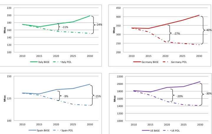
Figure 2 shows the primary consumption reductions in policy scenario for the three selected countries and for the EU as a whole. In 2020, looking at the values in Mtoe shows that the baseline scenario is consistent with scenario “Assenza di misure” in the Italian National Energy Strategy (Strategia Energetica Nazionale, SEN), which is lower than the Primes 2007 baseline (European Commission, 2008). The reduction in primary energy consumption would be higher in Germany and lower in Spain, consistently with the committement set by national energy policies. In 2030, the policy scenarios would allow Italy to stay on a decreasing pattern, and the same is true for Germany and Spain. At EU level, in 2020 the 20% consumption reduction objective would reached, and in 2030 primary energy consumption would be reduced by 30%, even more than the 27% objective set

in the October Communication8.

8_{Differently from the emission reduction objective which is set referring to the 1990 levels, the 27% energy efficiency}

(21)

20

Figure 2 – Primary energy consumption in baseline and policy scenarios

The reductions in primary energy consumption are reflected in the trends followed by CO2

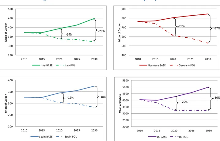
emissions, which would allow the EU to reach the 20% reduction target relative to the baseline in 2020, and of 36% in 2030 (Figure 3). In particular, at country level this would translate in significant reductions for all the three examined countries, by 36% in Germany, 14% in Italy and 12% Spain in 2020. The changes would become more important in 2030.

1000 1200 1400 1600 1800 2000 2200 2010 2015 2020 2025 2030 M to e UE BASE UE POL 100 120 140 160 180 200 220 2010 2015 2020 2025 2030 M to e

Italy BASE Italy POL

100 125 150 2010 2015 2020 2025 2030 M to e

Spain BASE Spain POL

200 250 300 350 400 450 2010 2015 2020 2025 2030 M to e

Germany BASE Germany POL

-11% -9% -27% -20% -15% -30% -24% -40%

(22)

21

Figure 3 – Carbon emissions in baseline and policy scenarios

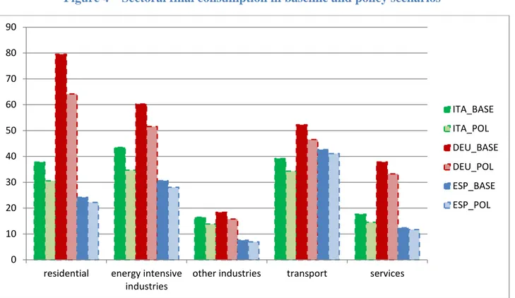
Figure 4 provide more details relative to the baseline level of sectoral final consumption in the three examined countries, and also relative to the corresponding reduction arising in policy scenario.

2000 2500 3000 3500 4000 4500 5000 5500 2010 2015 2020 2025 2030 M to n o f C a rb o n UE BASE UE POL 250 300 350 400 450 500 2010 2015 2020 2025 2030 M to n o f C a rb o n

Italy BASE Italy POL

200 250 300 350 400 2010 2015 2020 2025 2030 M to n o f C a rb o n

Spain BASE Spain POL

400 500 600 700 800 900 2010 2015 2020 2025 2030 M to n o f C a rb o n

Germany BASE Germany POL

-18% -12% -20% -14% -29% -37% -28% -36%

(23)

22

Figure 4 – Sectoral final consumption in baseline and policy scenarios

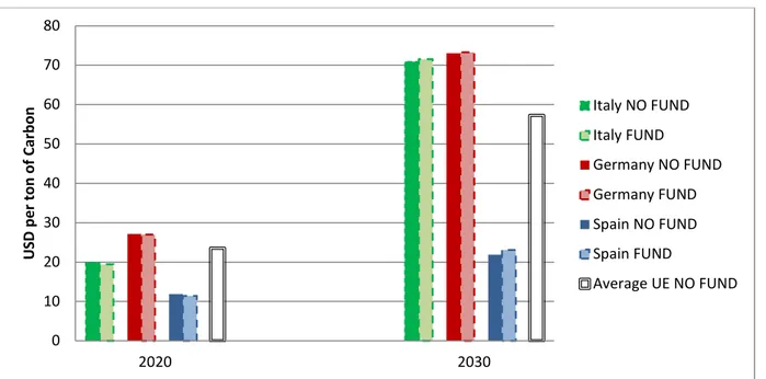
Figure 5 shows the carbon tax computed by the model, both in terms of national values and average

value for the EU9. In 2020, the carbon tax is equal to almost 24 USD per ton of carbon on average

in the EU, slightly higher than the projections included in the Directive 27/2012 Impact

Assessment. The value would increase significantly in 2030 up to 57 USD per ton of carbon, a

value in line with the projections included in the Communication (2014)15 Impact Assessment. As for individual countries, in 2020 Italy would be the closest to the EU average, showing a carbon tax slightly lower, whereas the tax would be higher than the EU average in Germany and considerably lower in Spain. By contrast, in 2030 the carbon tax would become higher than the EU average in Italy also, where a level comparable to the German carbon tax would be reached. The value for Spain would remain well below the EU marginal cost of emission reduction. This could be due both to a relatively lower emission target and to the existence of lower cost reduction opportunities, for example linked to the use of RES.

It is interesting to note that, until 2020, in the FUND scenario a decreasing impact on carbon tax is observed, although limited in its extent. On the other hand, after 2020 the fund would have an increasing impact on the carbon tax value. This pattern seems to suggest that in an initial period the fund would decrease the marginal cost of achieving the reduction target, whereas later on it would help in promoting energy efficiency interventions, but the cost of the remaining interventions would

9_{These carbon taxes may be interpreted as the marginal cost associated to the achievement of CO}

2 emission reduction

objectives, at national and EU level (hypothesising that no emission trading scheme is in place).

0 10 20 30 40 50 60 70 80 90

residential energy intensive industries

other industries transport services

ITA_BASE ITA_POL DEU_BASE DEU_POL ESP_BASE ESP_POL

(24)

23

become higher, since the lower-cost emission reduction opportunities had been already exploited. In the FUND scenario, the 80% of the revenue from carbon taxation is assumed to be earmarked to the national fund for energy efficiency and to be invested in energy efficiency interventions.

Figure 5 – Carbon tax values in policy scenarios

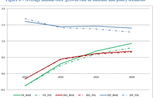
Figure 6 compares the annual GDP growth rate in the baseline and policy scenario, showing how in both Italy and Germany there would be an increasing trend, which would be lowered in the emission reduction scenario. The policy impact would be lower in Germany, and slightly more important in Italy. By contrast in Spain a decreasing trend is observed both in baseline and policy. It is interesting to note that, in this country, the implementation of the fund would imply an expansive impact in the first year, namely the annual growth rate would be higher in the policy than in the baseline scenario. 0 10 20 30 40 50 60 70 80 2020 2030 U S D p e r to n o f C ar b o n Italy NO FUND Italy FUND Germany NO FUND Germany FUND Spain NO FUND Spain FUND Average UE NO FUND

(25)

24

Figure 6 – Average annual GDP growth rate in baseline and policy scenarios

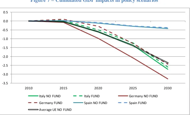
The information on GDP can be looked in another perspective, namely in cumulated terms. Figure 7 shows the cumulated impacts for the three countries considered, calculated as difference relative to the baseline. In Spain relatively smaller impacts are observed, while the strongest impacts would arise in Germany. For all countries, the FUND scenario would imply an improvement in the GDP trend, which would become less negative, especially for Italy and Spain, where an expansive impact is even observed in the first year after the fund introduction. In the EU as a whole, a GDP contraction equal to 0.6% is observed in 2020, which increases to 2.4% in 2030. A GDP contraction is reported also in Communication (2014)15 Impact Assessment.

-0.5 0.0 0.5 1.0 1.5 2.0 2015 2020 2025 2030

(26)

25

Figure 7 – Cumulated GDP impacts in policy scenarios

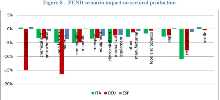
The macroeconomic impacts of policy scenarios can be analysed also looking at sectoral production and employment. Also in Figure 8 and 9 the impacts are calculated relative to the baseline, with the value of sectoral production expressed in current terms. Only results from the FUND scenario are shown, and it should be kept in mind that the impacts in the NO FUND scenario would generally be more important, as already shown relative to GDP. Sectoral production would decrease in all energy intensive sectors (Figure 8), with few exceptions in Spain and in Italy, the most important ones in iron and steel, non metallic minerals and textile sectors.

-3.5 -3.0 -2.5 -2.0 -1.5 -1.0 -0.5 0.0 0.5 2010 2015 2020 2025 2030

Italy NO FUND Italy FUND Germany NO FUND

Germany FUND Spain NO FUND Spain FUND

(27)

26

Figure 8 – FUND scenario impact on sectoral production

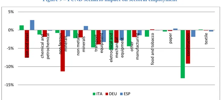
Consistently with production, employment would decrease in almost all energy intensive sectors (Figure 9). Since there is no unemployment in GDyn-E, after the policy interventions labour force would only be reallocated among sectors, and it would not decrease in absolute terms. The increase in employment of iron and steel sector in Italy and Spain could be due to the higher demand of the corresponding output to develop energy efficiency technologies and services, and the same could apply to non metallic minerals sector in Spain. Such a pattern has already been identified in Communication (2014)15 Impact Assessment, where the application of two different models, GEM-E3 and E3ME, shows that energy efficiency policies lead to increased demand in sectors providing goods and services to be used in energy efficiency interventions.

-20% -15% -10% -5% 0% 5% ir o n a n d s te e l ch e m ic a l a n d p e tr o ch e m ic a l n o n f e rr o u s m in e ra ls n o n m e ta ll ic m in e ra ls tr a n sp o rt e q u ip m e n t e le tr o cn ic a l a n d m e ch a n ic a l e q u ip m e n t o th e r m a n u fa ct u ri n g fo o d a n d t o b a cc o p a p e r co n st ru ct io n te xt il e

(28)

27

Figure 9 – FUND scenario impact on sectoral employment

Figure 10 and 11 analyse the impact on trade balance for the three countries in which the national fund for energy efficiency is introduced. International trade impacts appear to be highly differentiated by country. Germany shows higher impacts on exports, in particular in iron and steel, non ferrous metals and non metallic minerals sectors. In Italy, impacts on exports would be smaller, namely exports would decrease less than in Germany, and in more than one case they would even increase, in a significant way for other manufacturing and textile sectors. Consistently with what already observed for GDP, impacts in Spain would be less relevant. Looking at imports, Italy is the country in which the reduction in imports would be more relevant, followed by Germany and Spain, and this pattern implies a relatively better impact on the net trade balance value.

Figure 10 – FUND scenario impact on exports

-15% -10% -5% 0% 5% ir o n a n d s te e l ch e m ic a l a n d p e tr o ch e m ic a l n o n f e rr o u s m in e ra ls n o n m e ta ll ic m in e ra ls tr a n sp o rt e q u ip m e n t e le tr o cn ic a l a n d m e ch a n ic a l e q u ip m e n t o th e r m a n u fa ct u ri n g fo o d a n d t o b a cc o p a p e r co n st ru ct io n te xt il e

ITA DEU ESP

-20% -15% -10% -5% 0% 5% 10% ir o n a n d s te e l ch e m ic a l a n d p e tr o ch e m ic a l n o n f e rr o u s m in e ra ls n o n m e ta ll ic m in e ra ls tr a n sp o rt e q u ip m e n t e le tr o cn ic a l a n d m e ch a n ic a l e q u ip m e n t o th e r m a n u fa ct u ri n g fo o d a n d t o b a cc o p a p e r co n st ru ct io n te xt il e

(29)

28

Figure 11 – FUND scenario impact on imports

To help figuring out an overall picture, Figures 12–14 provide country data on different variables combined all together. More information could be found in the Tables collected in the Annex.

Figure 12 – Policy scenario impacts on selected variables: Italy

Focusing on Italy, in line with the pattern already described for GDP, in the FUND scenario an improvement of the impacts on value added is observed, at total and sectoral level. The two policy scenarios would imply a reduction of total value added equal to around 1% relative to the baseline in 2020, and equal to almost 6% in 2030. In some sectors, such as transport equipment and machinery, the emission reduction target would imply relatively higher impacts, both in 2020 and 2030. -15% -10% -5% 0% 5% ir o n a n d s te e l ch e m ic a l a n d p e tr o ch e m ic a l n o n f e rr o u s m in e ra ls n o n m e ta ll ic m in e ra ls tr a n sp o rt e q u ip m e n t e le tr o cn ic a l a n d m e ch a n ic a l e q u ip m e n t o th e r m a n u fa ct u ri n g fo o d a n d t o b a cc o p a p e r co n st ru ct io n te xt il e

ITA DEU ESP

-11% -7% -10% -14% -1% -0.8% -2% -1% -3% -5% -24% -17% -21% -38% -5% -4% -4% -4% -7% -9% GIC TFC Energy intensity CO2 emissions Energy dependency GDP VA Employment Import Export 2020 FUND scenario wrt Baseline 2030 FUND scenario wrt Baseline

(30)

29

As for employment, also in this case the FUND scenario would produce an increase in total and sectoral occupation levels relatively to the NO FUND scenario in all the examined period. In the two scenarios, on average, employment would be lower than in the baseline, by around 1% in 2020 and 4% in 2030.

Looking at the net trade balance, the two policy scenarios would imply an improvement both in 2020 and 2030 relatively to the baseline. As stated in the Directive 27/2012, shifting to a more energy-efficient economy should also accelerate the spread of innovative technological solutions and improve competitiveness in several sectors related to energy efficiency. One of the drivers of this positive effect could be the decrease in energy imports due to the investments in energy efficiency, which will be commented below. In 2020, the net trade balance would worsen in the FUND scenario relatively to the NO FUND scenario due to an increase in imports. Part of this increase could happen thanks to energy efficiency investments: with the fund some industrial sectors would contract their production less, and for this reason would have a higher demand for intermediate imported goods. On the other hand, in 2030 the negative impact on trade balance would be eased, due to a diversified impact on exports. In particular, in specific sectors, such as iron and steel, transport equipment and electronic and machinery equipment, an increase in exports is observed relatively to the NO FUND scenario, which could result from the improvements in competitiveness of domestic industries associated to energy efficiency interventions.

In both policy scenarios, energy intensity would decrease and energy dependency would be reduced, confirming the multiple benefits of energy efficiency (IEA, 2014), in this case in terms of energy security. The introduction of the fund would entail a slightly higher decrease of total energy

intensity10. A similar pattern holds at sectoral level. On the contrary, energy dependence would not

be differentiated in the two policy scenarios, showing a reduction of 1% in 2020 and almost 5% in 2030.

Figure 12 shows a synthesis of the results just described for a selection of key variables. Further details can be found in Table A1 and A2 in the Annex, where all results are expressed in percentage changes relatively to baseline scenario.

10

It is worth to specify that total energy intensity is computed basing on primary energy consumption, whereas sectoral energy intensity basing on final energy consumption ( http://www.enea.it/it/comunicare-la-ricerca/le-parole-dellenergia/fonti-rinnovabili-scenari-e-politiche/intensita-energetica).

(31)

30

Figure 13 – Policy scenario impacts on selected variables: Germany

In Germany, as already observed for Italy, both policy scenarios would imply a contraction in GDP and in total and sectoral value added. In this case, the FUND scenario shows a strong improvement of the impacts on sectoral value added.

The same is true for total employment, for which in 2020 is observed a 1.4% decrease in NO FUND scenario which is lowered to 0.9% in the FUND scenario. In 2030 the impacts on total employment would be higher, equal to around -2%, but also in this case the fund would allow to ease the reduction, by 0.5 percentage points. At sectoral level, the fund expansive impact would be particularly pronounced on chemical and petrochemical sector.

As already observed for Italy, in Germany the impact of the two policy scenarios on net trade balance would be positive. Also in this case, the FUND scenario shows a worst international trade performance in 2020 relatively to the NO FUND scenario. An opposite pattern is observed in 2030, due to lower imports and a lower reduction in exports from chemical and petrochemical sector.

Similarly to Italy, in both policy scenarios energy intensity would decrease relative to the baseline, by around 27% in 2020 and almost 40% in 2030. The FUND scenario would produce slightly higher improvements in energy intensity than the NO FUND scenario. In specific sectors, such as transport equipment, machinery and services, such trend is more pronounced in all the examined period. Energy dependence would also decrease in the two policy scenarios, but it would not show a differentiation. -28% -15% -27% -36% -2% -0.2% -3% -0.9% -5% -6% -41% -27% -40% -49% -7% -1% -5% -2% -8% -10% GIC TFC Energy intensity CO2 emissions Energy dependency GDP VA Employment Import Export 2020 FUND scenario wrt Baseline 2030 FUND scenario wrt Baseline

(32)

31

The results outlined above are summarised in Figure 13, and further details can be found in Table A3 and A4 in the Annex.

Figure 14 – Policy scenario impacts on selected variables: Spain

In Spain, the expansive impact of the fund on GDP would be less important than in the other countries, and the same holds relatively to the impact on total and sectoral value added, in all the examined period. The reduction in total valued added would be less than 1% in 2020 and 1% in 2030. The highest impacts are observed in transport equipment and machinery, as in Italy.

The impacts generated by the emission targets on total employment would also be limited, implying a contraction equal to around 0.5% in 2020 and 0.7% in 2030. At sectoral level, the occupation change would be lower than in other examined countries, being never higher than 2% in 2020 and 3% in 2030. The FUND scenario would imply a very slight decrease of the impacts, in particular in machinery sector.

Consistently with other countries, the two policy scenarios would improve net trade balance in 2020 and 2030 relatively to the baseline. In 2020 the trade balance value would be almost the same in the two scenarios, while in 2030 it would be slightly better in the FUND scenario, due to a small increase in exports.

The energy efficiency targets would produce a decrease in energy intensity by almost 30% in 2002 and almost 40% in 2030. In the NO FUND scenario the reduction in energy intensity would be slightly higher in both years. As for energy dependence, it would increase relatively to the baseline, and the increase would be to some extent lower in the FUND scenario. An increasing pattern could

-15% -3% -29% -12% 28% -0.2% -1% -0.5% -3% -6% -9% -6% -39% -18% 36% -0.1% -2% -0.6% -4% -8% GIC TFC Energy intensity CO2 emissions Energy dependency GDP VA Employment Import Export 2020 FUND scenario wrt Baseline 2030 FUND scenario wrt Baseline

(33)

32

appear counterintuitive, but it should be considered that energy dependence is strictly related to the structural characteristics of economies, so different impacts could be observed in different countries. Further research would be needed to explain this result.

The results for Spain are summarised in Figure 14, and further details can be found in Table A5 and A6 in the Annex.

5 Conclusions

The analysis developed above has shown the macroeconomic impacts of the 2020 energy efficiency national indicative targets as well as those of the more recent EU 2030 objective. It has been highlighted how the information which can be provided by GDyn-E model is analogous to the one included in the Impact Assessment documents elaborated by European Commission. Although specific comparison with the results included in Directive 27/2012 Impact Assessment or Communication (2014)15 Impact Assessment was not performed due to differences in the modelling approach, GDyn-E model could be used in the future to provide further estimates of EU energy policy impacts on Italy and other member countries. These estimates could be put together with the existing ones in order to enlarge the range of medium-term impacts available in policy evaluation..

In the EU Impact Assessments the general equilibrium (top-down) model GEM-E3 is used together with the bottom-up model Primes, in which a wide range of energy technologies is included. The relatively good detail covered by GDyn-E in terms of energy consumption by source and sector is a key characteristic for developing a soft-linkage with technological bottom-up models such as Times-Italy. A first experiment has recently been elaborated for the DDP report (Virdis et al., 2015).

Certainly, further interventions can be realised to improve GDyn-E model and the provided scenarios, such as introducing an explicit consideration of renewable energy, developing sensitivity analysis and performing a decomposition analysis of model results. Such interventions would contribute to fully exploit the model potential and to strengthen the reliability of its output.

(34)

33

References

Antimiani A., Costantini V., Martini C., Salvatici L., Tommasino M.C. (2013), “Assessing alternative solutions to carbon leakage”, Energy Economics, 36, 299–311.

Antimiani A.,Costantini V., Martini C., Palma A. Tommasino, M. C. (2013), “The GTAP-E: Model Description and Improvements”, in The Dynamics of Environmental and Economic Systems. Innovation, Environmental - - Policy and Competitiveness. (Eds) Costantini V. and Mazzanti, pp. 3-24. Springer Book, Netherlands.

Burniaux, J.-M., Truong, T.P., (2002), “GTAP-E an energy-environmental version of the GTAP model”, GTAP Technical Papers, No. 16. Center for Global Trade Analysis, Purdue University, West Lafayette, Indiana, USA 47907-1145.

Costantini, V., D’Amato, A., Martini, C., Tommasino, C., Valentini, E., Zoli, M. (2013), “Taxing international emissions trading”, Energy Economics, 40, 609-621.

European Commission (2014), “EU Energy Transport and GHG emissions – Trends to 2050 –

Reference scenarios 2013”,

http://ec.europa.eu/energy/sites/ener/files/documents/trends_to_2050_update_2013.pdf

European Commission (2014), “Impact Assessment accompanying the document Communication from the Commission to the European Parliament and the Council Energy Efficiency and its contribution to energy security and the 2030 Framework for climate and energy policy”,

SWD(2014) 255 final,

https://ec.europa.eu/energy/sites/ener/files/documents/2014_eec_ia_adopted_part1_0.pdf

European Commission (2014), “A policy framework for climate and energy in the period from 2020

to 2030”, COM(2014) 15 final,

http://eur-lex.europa.eu/legal-content/EN/ALL/?uri=CELEX:52014DC0015

European Commission (2011), “Impact Assessment accompanying the document Directive of the European Parliament and of the Council on energy efficiency and amending and subsequently repealing Directives 2004/8/EC and 2006/32/EC” IA Directive, SEC(2011) 779 final,

https://ec.europa.eu/energy/sites/ener/files/documents/sec_2011_0779_impact_assessment.pdf

European Commission (2010), “Europe 2020 - A strategy for smart, sustainable and inclusive

(35)

34

European Commission (2008), “European Energy and Transport – Trends to 2030 – Update 2007”,

http://ec.europa.eu/energy/sites/ener/files/documents/trends_to_2030_update_2007.pdf

European Council (2014), “2030 Climate and Energy Policy Framework”, EUCO 169/14,

http://data.consilium.europa.eu/doc/document/ST-169-2014-INIT/en/pdf

Gaeta, M. and Baldissara, B. (2011), “Il modello energetico Times-Italia. struttura e dati versione

2010”, ENEA-RT-2011-09, http://opac22.bologna.enea.it/RT/2011/2011_9_ENEA.pdf

Golub, A. (2013), “Analysis of climate policies with GDyn-E”, GTAP Technical Paper 4292, Center for Global Trade Analysis, Department of Agricultural Economics, Purdue University,

https://www.gtap.agecon.purdue.edu/resources/download/6632.pdf

Hertel, T.W. (1997), “Global Trade Analysis: Modeling and applications”, Cambridge University

Press, Cambridge, https://www.gtap.agecon.purdue.edu/products/gtap_book.asp

Ianchovichina, E.,McDougall, R. (2001), “Theoretical Structure of Dynamic GTAP”, GTAP Technical Paper No. 17, Center for Global Trade Analysis, Department of Agricultural Economics,

Purdue University, https://www.gtap.agecon.purdue.edu/resources/res_display.asp?RecordID=480

IEA (2015), Policies and measures database – Energy efficiency,

http://www.iea.org/policiesandmeasures/energyefficiency/?country=Spain

IEA (2014), “Capturing the Multiple Benefits of Energy Efficiency”,

http://www.iea.org/publications/freepublications/publication/capturing-the-multiple-benefits-of-energy-efficiency.html

Italian Ministry of Economic Development (2014), National Energy Efficiency Action Plan 2014”,

http://www.efficienzaenergetica.enea.it/politiche-e-strategie-1/politiche-e-strategie-in-italia/paee/paee-2014.aspx

Italian Ministry of Economic Development (2013), “National Energy Strategy”,

http://www.sviluppoeconomico.gov.it/index.php/it/component/content/article?id=2029441:strategia

-energetica-nazionale-sen

Markandya, A., Antimiani A., Costantini V., Martini C., Palma, A., Tommasino M.C. (2015), “Analyzing Trade-offs in International Climate Policy Options: The Case of the Green Climate Fund”, World Development, 74, 93–107.

(36)

35

Martini, C. and Tommasino, M.C. (2011), “GTAP-DYN drivers for the EFDA-TIMES Model”,

Final Report EFDA Reference: WP 10-SER-ETM-7,

https://www.euro-fusion.org/wpcms/wp-content/uploads/2014/12/WP10-SER-ETM-7.pdf

Martini, C. and Tommasino, M.C. (2010) “General equilibrium modelling for energy policies

evaluation : the GTAP-E ITA model”, ENEA-RT-2010-10,

http://opac22.bologna.enea.it/RT/2010/2010_10_ENEA.pdf.

Narayanan, G., B., Aguiar A., and McDougall, R. (2012), “Global Trade, Assistance, and Production: The GTAP 8 Data Base”, Center for Global Trade Analysis, Purdue University,

https://www.gtap.agecon.purdue.edu/databases/v8/v8_doco.asp

Narayanan, B., Dimaran, B., McDougall, R. (2012), “GTAP 8 Data Base Documentation - Chapter

2: Guide to the GTAP Data Base”,

https://www.gtap.agecon.purdue.edu/resources/res_display.asp?RecordID=3777

OECD (2012), “Environmental Performance Reviews: Germany 2012”.

Truong, P. T. and Lee, H.-L. (2003), “GTAP-E Model and the ‘new’ CO2 Emissions Data in the GTAP/EPA Integrated Data Base – Some Comparative Results”, GTAP Resource #1296, Center for

Global Trade Analysis, Purdue University,

https://www.gtap.agecon.purdue.edu/resources/res_display.asp?RecordID=1296

Virdis, M. R., Alloisio, I., Borghesi, S., De Cian, E., Gaeta, M., Martini, C., Parrado, R., Tommasino, M. C., Verdolini, E. (2015), “Pathways to Deep Decarbonisation in Italy”,

http://deepdecarbonization.org/countries/#italy

Walmsley, T. L., Anguiar, A.H., Narayanan B. (2012), “Introduction to the Global Trade Analysis Projec and the GTAP Data Base”, GTAP Working Paper No. 67, Center for Global Trade Analysis,

(37)

36

Annex

Table A1 – Italy 2020 2020 Baseline 2020 Objectives wrt Baseline 2020 Objectives with fund wrt Baseline

Primary energy consumption (Mtoe) 176 -10.9% -11.0%

Final energy consumption (Mtoe) 137 -6.8% -6.6%

Gross Domestic Product (current USD

million) 2,149,183 -1.0% -0.8%

Total value added (current USD million) 1,942,176 -1.8% -1.6%

Sectoral value added (current USD million)

. chemical and petrochemical 68,033 -1.3% -1.3%

. transport equipment 83,690 -1.7% -1.5% . machinery 119,690 -1.8% -1.5% . food 73,202 -0.9% -0.8% . textile 66,690 0.3% 0.3% . services 1,064,160 -1.9% -1.6% Employment 821,155 -1.3% -1.1% Sectoral employment

. chemical and petrochemical 34,672 0.2% -0.1%

. transport equipment 44,946 -1.4% -1.2%

. machinery 71,524 -1.2% -1.0%

. food 24,936 -0.4% -0.3%

. textile 37,944 0.8% 0.7%

. services 423,349 -1.8% -1.6%

Energy intensity (Mtoe per USD) 81.9 -10.0% -10.2%

Sectoral energy intensity (Mtoe per USD)

. chemical and petrochemical 216.8 -3.0% -2.9%

. transport equipment 22.3 -0.8% -1.0%

. machinery 46.4 -5.5% -5.6%

. food 50.7 -6.1% -6.1%

. textile 36.2 -6.3% -6.3%

. services 14.8 -5.0% -5.1%

Net trade balance (current USD million) 11,522 25,642 24,607

Sectoral exports (current USD million)

. transport equipment 82,457 0.3% 0.4% . machinery 132,687 0.9% 0.9% . food 38,384 0.5% 0.4% . textile 65,949 2.7% 2.4% . services 84,007 1.0% 0.9% Energy dependency 0.73 -1.1% -1.1%

(38)

37 Table A2 – Italy 2030 2020 Baseline 2030 Objectives wrt Baseline 2030 Objectives with fund wrt Baseline

million) 2,765,528 -4.3% -4.1%

Total value added (current USD million) 2,523,591 -6.0% -5.9% Sectoral value added (current USD million)

. transport equipment 109,810 -5.7% -5.5% . machinery 144,060 -6.9% -6.7% . food 89,978 -3.0% -2.9% . textile 69,630 -0.9% -0.8% . services 1,348,025 -5.7% -5.6% Employment 1,002,926 -4.6% -4.5% Sectoral employment

. machinery 82,754 -5.6% -5.4%

. food 29,303 -1.8% -1.8%

. textile 37,958 0.1% 0.2%

. services 512,021 -5.4% -5.3%

. machinery 42.3 -13.7% -13.7%

. food 46.2 -15.4% -15.3%

. textile 34.3 -15.5% -15.4%

. services 13.1 -12.7% -12.7%

Net trade balance (current USD million) -151,235 -98,584 -98,807 Sectoral exports (current USD million)

. transport equipment 89,584 0.9% 1.0% . machinery 101,512 1.5% 1.6% . food 49,738 1.1% 1.2% . textile 54,578 5.3% 5.2% . services 92,489 2.5% 2.5% Energy dependency 0.81 -4.6% -4.6%

(39)

38

Table A3– Germany 2020

2020 Baseline 2020 Objectives vs Baseline 2020 Objectives with fund vs Baseline

million) 4,116,359 -0.9% -0.2%

. chemical and petrochemical 84,608 -1.4% 0.1%

. machinery 201,876 -0.7% -0.6%

. food 54,994 -0.1% 0.3%

. textile 18,706 0.6% 0.5%

. services 1,196,001 -1.7% -1.1%

. machinery 11.0 -10.0% -11.4%

. food 62.5 -15.9% -16.6%

. textile 31.5 -13.8% -14.4%

. services 16.6 -9.7% -10.9%

Net trade balance (current USD million) 26,413 69,561 62,605 Sectoral exports (current USD million)

. transport equipment 331,265 -0.1% -0.6% . machinery 363,940 2.7% 1.6% . food 68,452 -0.4% -0.6% . textile 40,717 0.8% 0.2% . services 137,748 1.9% 1.1% Energy dependency 0.61 -3.2% -2.0%

(40)

39

Table A4– Germany 2030

2030 Baseline 2030 Objectives wrt Baseline 2030 Objectives with fund wrt Baseline

million) 5,070,718 -2.0% -1.3%

. machinery 196,998 -3.7% -3.4%

. food 66,220 -0.1% 0.2%

. textile 19,728 -0.3% -0.1%

. services 1,412,487 -2.7% -2.2%

. machinery 10.1 -19.1% -20.1%

. food 58.1 -27.0% -27.6%

. textile 30.6 -23.5% -23.8%

. services 15.1 -18.2% -19.1%

Net trade balance (current USD million) -150,249 -94,982 -92,492 Sectoral exports (current USD million)

. transport equipment 363,179 -2.1% -2.2% . machinery 290,293 1.4% 0.9% . food 91,217 -1.5% -1.5% . textile 39,988 -0.7% -0.8% . services 155,263 1.0% 0.8% Energy dependency 0.65 -8.0% -7.0%

(41)

40 Table A5 – Spain 2020 2020 Baseline 2020 Objectives wrt Baseline 2020 Objectives with fund wrt Baseline

million) 1,428,364 -0.3% -0.2%

. transport equipment 57,297 -2.0% -1.8% . machinery 43,098 -1.6% -1.5% . food 39,097 -0.6% -0.5% . textile 21,524 -0.2% -0.2% . services 778,504 -0.8% -0.7% Employment 681,549 -0.6% -0.5% Sectoral employment

. chemical and petrochemical 23,973 0.2% -0.1%

. machinery 24,715 -1.5% -1.3%

. food 18,404 -0.3% -0.3%

. textile 12,240 -0.1% 0.0%

. services 406,812 -0.7% -0.7%

. machinery 35.5 -3.2% -3.0%

. food 58.6 -3.2% -3.0%

. textile 39.0 -2.8% -2.6%

. services 15.6 -2.2% -2.1%

Net trade balance (current USD million) 90,834 93,638 93,636 Sectoral exports (current USD million)

. transport equipment 93,938 -1.7% -1.5% . machinery 56,756 -1.1% -0.9% . food 31,844 -0.1% -0.1% . textile 23,440 0.5% 0.5% . services 116,822 -0.4% -0.3% Energy dependency 0.57 27.8% 27.6%