Point thermal transmittance of rib intersections in concrete sandwich wall panels

POINT THERMAL TRANSMITTANCE OF RIB INTERSECTIONS IN CONCRETE

SANDWICH WALL PANELS

Benedetti M.1, Gervasio P.2, Luscietti D.3, Pilotelli M.3, Lezzi A.M.3∗ ∗_{Author for correspondence}

1_{Dipartimento di Ingegneria dell’Informazione,}

2_{Dipartimento di Ingegneria Civile, Architettura, Territorio, Ambiente e di Matematica,} 3_{Dipartimento di Ingegneria Meccanica ed Industriale,}

Universit`a degli Studi di Brescia, via Branze 38, 25123 Brescia E-mail: adriano.lezzi@unibs.it

ABSTRACT

Concrete sandwich panels are widely used building elements. They are made by two reinforced concrete wythes separated by a layer of lightweight material: the central layer is inhomoge-neous due to the presence of concrete ribs which tie the exter-nal wythes and act as thermal bridges. Internatioexter-nal Standards allow to evaluate the average thermal transmittance of concrete sandwich panels as a linear combination of the transmittance of the solid concrete ribs and of the lightened parts - calculated as if the temperature field were 1D - and linear and point thermal transmittances associated with thermal bridges. In a recent work we have addressed the problem of finding an accurate correla-tion for prediccorrela-tion of linear thermal transmittance values. The goal was reached upon use of a fast and accurate Spectral Ele-ment Method. In this work we complete our study investigating the point thermal bridges and determining the associated point thermal transmittance. Point thermal transmittances in sandwich panels are associated with the concrete rib intersections, like in the four panel corners, and require 3D numerical simulations for their evaluation: the computational effort required to approxi-mate the point transmittance is much larger than that needed to estimate the linear one. For this reason we present and discuss a solution strategy based on the use of low-order polynomials (p = 4) on three grids of increasing refinement, starting from a very coarse one: results have been improved through an iterated application of Richardson extrapolation. This procedure assures a good trade-off between accuracy, as required by Standards, and computational cost. A dataset of 1080 point transmittance values is obtained varying systematically six geometrical and thermo-physical parameters. A simple power law correlation in terms of a single variable depending on linear transmittance of the inter-secting ribs is introduced and its accuracy assessed.

INTRODUCTION

Precast concrete sandwich wall panels allow fast and econom-ical constructions of buildings such as factories, warehouses, and malls. Since they are usually produced far from the construc-tion site, weight becomes a crucial point with regard to handling,

transportation, and installation issues. The easiest way to meet both the requirements of structure robustness and weight con-tainment, is to have a frame of concrete and fill the empty zones with lightweight materials like expanded polystyrene. In what follows this kind of panel will be referred to as LSP, precast con-crete Lightened Sandwich wall Panel. It is worth underlying that LSPs are not designed to be thermal efficient because the use of insulating slabs is aimed to reduce weight, reduction of the aver-age thermal transmittance is just a by-product effect.

In a LSP two prestressed concrete wythes are separated by a heterogeneous layer made by lightweight slabs and concrete ribs: so there are panel regions made of solid concrete which act as thermal bridges. In principle, computation of the thermal trans-mittance U of LSPs is not a critical issue: ISO 6946, ISO 14683, and ISO 10211 [1, 2, 3] describe accurate methods to do that. These methods require the knowledge of linear and point thermal transmittance associated with thermal bridges in LSPs. Their val-ues can be computed upon numerical simulations performed as described in ISO 10211. However, most panel manufacturers are SMEs (Small-Medium Enterprises) and their technical staff does not have either the know-how, nor the time to numerically com-pute values necessary to determine the transmittance U of their product range: they consider much more convenient the usage of transmittance catalogues or correlations, easily implemented in a spreadsheet or in an in-house code.

In a previous paper [4] we addressed the problem of finding an accurate correlation for prediction of linear thermal transmit-tance values of LSPs. In the present work we complete our study investigating the point thermal bridges in LSPs and determining the associated point thermal transmittance.

Point thermal bridges in LSPs coincide with concrete rib in-tersections, like in the four panel corners. ISO 14683 states that, in general, the effect of point thermal bridges ”insofar they result from the intersection of linear thermal bridges”, can be neglected [2, Clause 4.2]. In past years, we had to evaluate in a few real cases point thermal bridge contribution in LSPs and found that it accounted for up to 2%, approximately. Besides, the

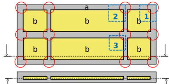
associ-b b b a b b b 1 2 3

Figure 1. Plan and section view of a LSP: a, solid concrete sec-tion; b, lightened section. Thick lines and open circles indicate linear and point thermal bridges, respectively. Domains 1, 2 and 3 are examples of 3D models used in numerical simulations. ated point transmittances were negative: neglecting them implied overestimating panel transmittance U . In this work we check the correctness and the generality of the latter conclusion, on the ba-sis of a systematic study of point transmittance as a function of concrete and lightweight material conductivities and panel geo-metrical parameters.

Evaluation of point thermal transmittance requires 3D numer-ical simulations, besides the knowledge of linear transmittance associated with the intersecting concrete ribs. As in [4] we use a conformal quadrilateral Spectral Element Method (SEM): the computational effort required to approximate point transmit-tances is much larger than that needed to estimate linear ones. That forces us to use coarse meshes and to approximate the tem-perature field in each mesh element with low-order polynomi-als, but with the major drawback of loss of accuracy. Here we present and discuss a solution strategy that allows to by-pass this problem. The numerical problem is solved on three grids of in-creasing refinement upon use of low-order polynomials (p = 4): results are extrapolated by Richardson method [5, 6]. This pro-cedure assures a good trade-off between accuracy, as required by International Standards, and computational cost.

A dataset of point transmittance values is obtained varying systematically material conductivities and thickness of external and central layers, for the most frequent pairs of rib widths in current panel production. We propose a simple power law cor-relation in terms of a new variable depending on linear transmit-tances and concrete wythes thickness. This correlation allows to estimate point transmittances within a relative error of ±10% which is intermediate between the typical accuracy of numeri-cal numeri-calculation of linear thermal transmittance (±5%) and that of linear thermal bridge catalogues (±20%)[2, Clause 5.1].

To our knowledge, in literature there are only a few other stud-ies on point thermal bridges in precast concrete panels and none of them is concerned with evaluation of point transmittance asso-ciated with rib intersections. Studies [7, 8, 9] do consider point transmittances, but they are concerned with the effect of metal connectors used to tie the concrete wythes in insulated sandwich wall panels.

AVERAGE THERMAL TRANSMITTANCE OF A LIGHT-ENED SANDWICH PANEL

The average thermal transmittance U of a wall panel is defined as U = q/A ∆T where q is the heat flow rate through the panel, ∆T is the temperature difference between the internal and the external environments separated by the panel, and A is the panel area. The four panel edges are considered adiabatic.

Although q could be calculated upon numerical solution of the conduction equation for the entire panel, International Standards [2, 3] suggest a more efficient method based on analytical and numerical solutions for a limited number of parts of the panel. Following this approach U is written as,

U= q A ∆T = 1 A

∑

_i AiUi+

∑

_j ljψj+

∑

_k nkχk ! (1)

In Eq. (1) Aiand Uiare area and thermal transmittance of the i-th sectionof the panel; ljand ψjare lenght and linear transmittance of the j-th linear thermal bridge; nkand χkare number and point transmittance of the k-th point thermal bridge. Following ISO 6946 [1, Clause 6.2.2], here section denotes a panel part made of thermally homogeneous layers. As clearly shown in Figure 1, a LSP is made of two sections: the solid concrete part, correspond-ing to ribs (section a); and the three-layer lightened part, made of the concrete wythes and the lightened layer that separates them (section b).

The thermal transmittance of the two sections, Uaand Ub, is easily calculated in terms of surface resistances, Rseand Rsi, and of thermal resistances of the homogeneous layers. Therefore, the first sum in Eq. (1), ∑iAiUirepresents the transmission heat coefficient through the panel as if the sections were thermally insulated one from the other, and the temperature field were 1D within each section.

The other two sums, ∑jljψj and ∑knkχk, represent the cor-rections associated with linear and point thermal bridges, that is with the regions where the temperature field is 2D and 3D.

In LSPs, the temperature field is closely approximated by a 2D field near the interfaces between concrete ribs and lightweight slabs (thick lines in Figure 1), whereas it is fully 3D in a neigh-borhood of the intersections of ribs (open circles in Figure 1).

The linear thermal transmittances ψjmust be evaluated upon solving the conduction equation on 2D domains as described in [4]. Evaluation of the point thermal transmittances χk– which is the goal of this study – requires solution of the conduction equa-tion on proper 3D domains which represent panel parts centered around rib intersections. These 3D geometrical models must be identified in accordance with ISO 10211.

POINT TRANSMITTANCE CALCULATION Problem description

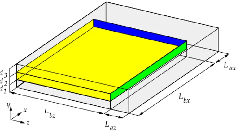
In Figure 2 it is sketched the 3D model used to determine point thermal transmittance values: it represents the part of a panel near the intersection of two ribs. The L-shaped region formed

L x z y d d d₁2 3 L_ax L_bz az L_bx

Figure 2. The computational domain Ω, the intersecting ribs form two linear and one point thermal bridges. The linear ther-mal transmittances are considered as associated with the blue (ψx) and green (ψz) interfaces.

by the intersecting ribs, represents the solid concrete section a, whereas the three-layered region is the lightened section b.

The 3D geometrical model coincides with the parallelepiped Ω of sides Lx= Lax+ Lbx and Lz= Laz+ Lbz, and height (panel thickness) d = d1+ d2+ d3. d1and d3denote the thickness of the external and internal wythe, respectively, whereas d2is the ligthweight material thickness.

On the domain boundaries the following conditions must be satisfied. On the external and internal surfaces ∂Ωe(y = 0) and ∂Ωi(y = d) Robin condition is imposed. The heat transfer from surface ∂Ωeto the external environment at temperature Teis char-acterized by a heat transfer coefficient heand a surface resistance Rse= 1/he. Internal environment temperature Ti, heat transfer coefficient hi, and surface resistance Rsi= 1/hicharacterize heat transfer to the internal surface ∂Ωi.

Planes x = 0, x = Lx, z = 0, and z = Lz are cut-off planes as defined in ISO 10211 [3, Clause 5.2], which coincide with adiabatic surfaces: the union of all adiabatic lateral surfaces will be denoted ∂Ωa.

Boundaries x = Lxand z = Lzbelong to either an adiabatic lat-eral surface of the panel (as in domains 1 and 2 in Figure 1) or a symmetry plane of an internal rib (as in domains 2 and 3 in Fig-ure 1): therefore Lax and Lazare either the width of a bounding rib or the half-width of an internal rib.

Boundaries x = 0 and z = 0 are placed so far from the inter-section that the temperature field on them is 2D for all practical purposes. According to ISO 10211 the distances Lbxand Lbz be-tween the cut-off planes and the point thermal bridge must be larger or equal to max(1 m, 3d), where d is the total thickness of the panel.

Denoting q the heat flux through the 3D domain Ω, Eq. (1) simplifies as follows,

q

∆T = AaUa+ AbUb+ Lbzψx+ Lbxψz+ χ, (2) where Aa+ Abis equal to the area of surfaces ∂Ωeand ∂Ωi. ψx and ψzare the linear transmittances associated with the interfaces

between concrete and lightweight material that are highlighted in blue and green, respectively, in Figure 2.

Upon numerical evaluation of q and ψx and ψz (see [4]) the point transmittance χ associated with the rib intersection mod-elled in Figure 2, can be computed as

χ = q

∆T − (AaUa+ AbUb+ Lbzψx+ Lbxψz) (3)

Input data

The point transmittance χ as defined by Eq. (3) depends on several parameters: geometrical, Lax, Laz, Lbx, Lbz, d1, d2, d3; and thermophysical, λco, λlw, Rse, Rsi.

In this study Rse, Rsi, Lbx, and Lbzare fixed, and χ is computed for varying values of the other variables. The surface resistances are set equal to the conventional values prescribed by ISO 6946 [1, Clause 5.2]: Rse= 0.04 m2K/W and Rsi= 0.13 m2K/W.

As observed in [4] linear transmittance ψ associated with a concrete rib tends asymptotically to a constant value as the lightweight slab length increases (Lbx and Lbzin Figure 2). As a matter of fact the growth is rapid: for length larger than 0.25 m the value of ψ is hardly distinguishable from the asymptotic value. Since in real panels the lightweight slab length and width are rarely smaller than 0.5 m, the asymptotic value only is needed for all practical purposes. A similar behaviour is expected to characterize the dependence of χ on Lbx and Lbz: therefore, fol-lowing ISO 10211, in all computations we set Lbx= Lbz= 1 m.

In [4] linear transmittance ψ were computed for about 38,000 different combinations of (Lax, d1, d2, d3, λco, λlw). Due to the larger computational cost of 3D simulations, here χ has been cal-culated for a subset of that dataset. In particular, only three val-ues for both concrete and lightweight material conductivity have been considered: λco = 1.6, 2.0, and 2.4 W/m K; λlw= 0.02, 0.04, and 0.06 W/m K.

The dependence of point transmittances on solid concrete sec-tionwidths Lax and Lazis similar to the one on Lbx and Lbz: it attains its asympotic value for widths larger than 0.2 m, approx-imately. Here we study the three most frequent values of rib width or half-width: 0.05, 0.10, and 0.20 m. In addition, we compute also the asymptotic cases which can be approximated setting widths equal to 1 m.

W.r.t. Figure 2, for symmetry reasons the value of χ is invari-ant when Laxand Lazcommute, thus only combinations Lax≤ Laz need to be considered.

In current production of LSPs the concrete wythes have usu-ally the same thickness, therefore analysis has been restricted to the symmetric case d1= d3. Three values of wythe thickness have been considered: 0.04, 0.06, and 0.08 m. They are the most frequent for panels of total thickness less than or equal to 0.24 m. Thickness of the lightened layer, d2, has been varied among: 0.04, 0.06, 0.08, 0.12, and 0.16 m. However, the following con-straint on panel total thickness has been imposed: d ≤ 0.24 m: only 12 combinations of values of d1and d2satisfy this condi-tion.

1080 numerical estimates of χ have been obtained upon vary-ing (Lax, Laz, d1, d2, λco, λlw) as specified above.

NUMERICAL SOLUTION

The conduction problem described in the previous section is solved through Spectral Element Methods (SEM). SEM are high accurate methods designed to discretize partial differential equa-tions. Their best performance (in terms of computational effi-ciency) is achieved when the differential problem is set on carte-sian geometries, exactly as in the problem we are dealing with, since SEM exploit the tensorial structure of the basis functions. The accuracy of SEM is restricted by the regularity of the data: the thermal conductivity and the prescribed boundary conditions. A brief description of SEM as applied to transmittance computa-tion in LSPs can be find in [4, Sec. 4], whereas for an in-depth description of SEM and of their use to approximate partial differ-ential equations, we refer, e.g., to [10, 11]. Here we present only features and terms necessary to understand the solution strategy adopted.

To approximate the temperature field T inside the panel the computational domain Ω is partitioned in Ne non-overlapping parallelepiped Qk (also named elements) of size h (tipically h denotes the diagonal), such that two adjacent elements share a vertex, an edge or a complete face. Such a partition will be de-noted by

_Q

_h=SNe

k=1Qk. We accept that the elements Qkcan have different size h_k, in such a case we set h = max

k hk.

Given a partition

Q

hof Ω we look for an approximation Th of T that is globally continuous on Ω and locally (that is in each element Qk) is a polynomial of degree p with respect to each vari-able. If the surfaces of discontinuity of the thermal conductivity do not cut any element Qk, it can be proved that the discrete solu-tion Thconverges to T when the mesh size h tends to zero and/or the polynomial degree p grows to infinity.

Once the discrete temperature Th is available, the heat flux through surfaces ∂Ωiand ∂Ωecan be computed by the following formulas: qi,h= Z ∂Ωi λco ∂Th(x) ∂n d∂Ω = Z ∂Ωi hi(Ti− Th)d∂Ω, qe,h= − Z ∂Ωe λco ∂Th(x) ∂n d∂Ω = Z ∂Ωe he(Th− Te)d∂Ω. (4)

qi,h and qe,h are the discrete approximation of the heat flux through Ω, q, that is required to calculate the point transmittance χ by Eq. (3). In particular, qi,h→ q and qe,h→ q when h → 0 and/or p → ∞. The SEM has been implemented in MATLAB. Discretization strategies

In order to get a good trade-off between accuracy and compu-tational time one has to choose properly the partition

Q

hand the polynomial degree p.

For each set of data, and any fixed p, the discrete fluxes, Eq. (4), have been computed for three different meshes:

Q

h (named coarse),

_Q

_h/2 (medium), and

_Q

_h/4(fine). Therefore, the

corresponding point transmittances χh,p, χh/2,p, and χh/4,p have been evaluated by using Eq. (3), in which q is replaced by its discrete counterpart qh= (|qi,h| + |qe,h|)/2.

Finally, χh,p, χh/2,p, and χh/4,pare used to better estimate the point transmittance χ through the Richardson extrapolation tech-nique (see, e.g. [6, Sec. 9.6]), that in our case (with data from three different meshes and the parameter h that is halved at each step) reads

χe,p=

8χh/4,p− 6χh/2,p+ χh,p

3 . (5)

In view of the convergence estimate of Richardson extrapola-tion (see, e.g., [6, Eq. (9.35)]), there exists a positive constant C, independent of h, but possibily depending on p such that |χe,p− χ| ≤ C(p)(h/4)3. The Richardson extrapolation turns out to be very efficient to our purpose. As a matter of fact, even if the SEM appproximation error vanishes as h when h → 0 in view of the low regularity of the thermal conductivity, Richardson ex-trapolation allows to gain third order accuracy w.r.t. h by using a set of three meshes of moderate sizes h, h/2, and h/4, instead of a unique mesh with a very small mesh-size, that would require very large computational effort.

In our simulations we have chosen to use polynomial degree p= 4. This choice is motivated by several numerical tests, car-ried out to measure both the computational effort required to solve the linear system associated with the SEM discretization of the conduction problem, and the accuracy of the computed point transmittance.

As test case to study discretization error and computational effort, we have chosen the case: Lax= Laz= 0.05 m, d1= d3= 0.06 m, d2= 0.12 m, λc= 2.0 W/m K, λlw= 0.04 W/m K, and on the associated geometry we have designed the following partitions.

The coarse mesh

_Q

_his obtained by defining 6 × 4 × 6(= 144) elements with side sizes hx= [0.6, 0.2, 0.1, 0.05, 0.05, | 0.05], hy= [0.06, | 0.06, 0.06, | 0.06], and hz = hx. Vertical pipes highlight where the thermal conductivity is discontinuous. The ratio between the maximum and the minimum size hk is about 10, with maxkhk' 0.85 and minkhk' 0.09. The medium mesh

Q

h/2is obtained by halving (along each direction) any element of

Q

h, therefore we have 12 × 8 × 12(= 1152) elements; while the finemesh

Q

h/4is obtained by halving (along each direction) any element of

Q

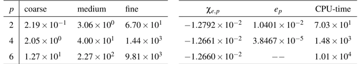
h/2, here we have 24 × 16 × 24(= 9216) elements.

The CPU-times (in seconds) needed to compute the tempera-ture field on an Intel i5-3470 4core, 64bit, 3.6GHz and 8GB of RAM, are reported in Table 1, left, for p = 2, . . . , 6 and the three partitions

Q

h,

Q

h/2and

Q

h/4. Least square approximation of the measured values provides CPU-time' 10−7p5.6N_e1.7s. We con-clude that a large computational effort is required when either moderate or large p is used.

To measure the accuracy of our numerical results, we compute the Richardson extrapolation of the point transmittance χe,p, for any p = 2, 4, 6, as well as the relative error w.r.t. χe,6(our best

p coarse medium fine 2 2.19 × 10−1 3.06 × 100 6.70 × 101 4 2.05 × 100 4.00 × 101 1.44 × 103 6 1.27 × 101 2.27 × 102 9.81 × 103 χe,p ep CPU-time −1.2792 × 10−2 1.0401 × 10−2 7.03 × 101 −1.2661 × 10−2 3.8467 × 10−5 1.48 × 103 −1.2660 × 10−2 −− 1.01 × 104

Table 1. At left, CPU-time in seconds needed to compute the temperature by SEM discretization. At right, the Richardson extrapolation of the point transmittances for different values of p, the errors w.r.t. the best computed value χe,6, and the CPU-times (in s)

estimate), i.e.,

ep=

|χe,p− χe,6| |χe,6|

. (6)

The computed point transmittances χe,p, the errors (6) and the CPU-times needed to estimate χe,p (i.e. the total CPU-time needed to compute the discrete temperature on all three meshes) are shown in Table 1, right. We conclude that the best compro-mise, obtained by minimizing both the CPU-time and the error is achieved for p = 4.

RESULTS AND DISCUSSION

1080 numerical estimates of χ have been obtained varying six parameters:

χ = χ(Lax, Laz, d1, d2, λco, λlw). (7)

The interval spanned by χ over the set of input data ranges between −4.38 × 10−2 and −0.48 × 10−2 W/K: all values are negative. There is no evidence that the dependence of χ on some of the variables could be neglected because it is much weaker than others.

At the beginning of this study we planned to develop an arti-ficial neural network (ANN) for prediction of χ, as we did for ψ in [4]. However, in [4] to train an ANN able to model correctly the dependence on Lawe had to obtain values of ψ for more than ten Labetween 0.05 and 1 m. In this study we could not afford the computational cost of tens of (Lax, Laz) pairs. Nor it seemed useful to develop an ANN for each pair (Lax, Laz) investigated. A different approach was followed.

According to ISO 14683 the point thermal bridge stud-ied here can be considered as the intersection of two linear bridges associated with transmittances ψx(Lax, d1, d2, λco, λlw) and ψz(Laz, d1, d2, λco, λlw)1. We asked ourselves whether the dependence of χ on the six variables could be captured to some extent by ψx and ψz, that is whether χ depend implicitly on (Lax, Laz, d1, d2, λco, λlw) through ψxand ψz:

χ = g(ψx, ψz). (8)

1_{Variable d}

3is not listed since we are considering only the case d3= d1.

For simmetry reason in Eq. (8) ψxand ψzmust commute, that is ghas to depend on commutative functions of ψxand ψz, such as ψxψz, ψx+ ψz, etc.

As a matter of fact, if computed values of χ are plotted versus ψxψzdata tend to fall within a smooth narrow region of increas-ing width for increasincreas-ing ψxψz. Data dispersion depends on the original variables, but dependence on d1seems stronger. After a few trials we came up with the following new variable

ξ = ψxψz p

2d1 (9)

for which dispersion is substantially reduced (see Figure 3). In Eq. (9) the factor 2 multiplying d1has been introduced because we believe that for the more general case d36= d1, variable ξ should be defined as ξ = ψxψz

√ d1+ d3.

Upon fitting data with a power law, the following correlation for point transmittance has been obtained:

χc(ξ) = −0.4391 ξ0.7055 (10)

where all quantities are in SI units.

For all practical purposes Eq. (10) supplies a rather good es-timate of χ when the linear transmittances associated with the intersecting ribs are known. In Figure 4 the point transmittance estimated by correlation (10), χc, is plotted versus the computed value χ: 97% of estimates fall within ±10% band.

Eq. (10) on average neither overpredict nor underpredict sig-nificantly χ, since the mean relative deviation, MRD, is equal to 0.09%. Dispersion of predicted values is limited since the stan-dard deviation, SD, is equal to 4.5%. Here, SD is defined in terms of relative deviation RD= (χc− χ)/χ: SD = s 1 N− 1

∑

_i (RDi− MRD) 2_.

As mentioned in the Introduction the relative contribution of point thermal bridges to the average panel transmittance U (term ∑knkχk in Eq. (1)) is up to 2%, approximately. Therefore the error introduced upon use of correlation (10) is up to 0.2% of U . CONCLUSIONS

This paper deals with the problem of determining point ther-mal transmittance associated with rib intersections in LSPs.

To-ξ[W2_/m3/2_K2_] 0 0.01 0.02 0.03 0.04 χ [W /K ] -0.05 -0.04 -0.03 -0.02 -0.01 0 −0.4391 ξ0.7055

Figure 3. All computed values of χ vs. the variable ξ = ψxψz

√

2d1. Solid line: least square approximation of data through a power law

|χ| [W/K] 0 0.01 0.02 0.03 0.04 0.05 |χ c | [W /K ] 0 0.01 0.02 0.03 0.04 0.05 −10% +10%

Figure 4. Comparison between correlation predictions, |χc|, and computed data χ: 97% of estimates fall within ±10% band gether with results presented in [4] it allows accurate calcula-tion – within ±1% – of nominal average thermal transmittance of LSPs according to current International Standards [1, 2, 3].

To reach this goal a dataset of point thermal transmittance as-sociated with rib intersections of LSPs has been built through nu-merical simulations. 1080 data have been obtained as a function of six parameters: rib widths, thickness of the concrete wythes and of the internal layer, concrete and lightweight material con-ductivity. The parameters span a range of values typical of cur-rent LSPs production. In general, ISO 14683 allows to omit point thermal bridge contribution to LSPs transmittance. For the input

data investigated here it is shown that this contribution is always negative: one stays on the safe side neglecting it when evaluating thermal performance of LSPs. Besides, point transmittance val-ues are rather small, their order of magnitude being 10−2W/K.

Accurate calculation of such a small quantity through numer-ical solution of heat conduction equation in a 3D domain has been tricky and required a solution strategy based on Richardson extrapolation. This procedure allowed to determine point trans-mittance values with a relative error which is about 10−4.

Finally, an explicit correlation is proposed for prediction of point transmittance. Although data show a significant depen-dence of χ on each of the six variables mentioned above, we manage to find a simple power law correlation which allows to calculate χ as a function of a single variable, ξ = ψxψz

√ 2d1. The correlation has standard deviation equal to 4.5% and predicts more than 97% of computed data within ±10%. It represents a good practical tool, easily implemented in a spreadsheet or in an in-house code for calculation of U .

REFERENCES

[1] ISO 6946. Building components and building elements -Thermal resistance and thermal transmittance - Calcula-tion method. 2007.

[2] ISO 14683. Thermal bridges in building construction - Lin-ear thermal transmittance - Simplified methods and default values. 2007.

[3] ISO 10211. Thermal bridges in building construction -Heat flows and surface temperatures - Detailed calcula-tions. 2007.

[4] Luscietti D., Gervasio P., and Lezzi A.M. J. Phys.: Conf. Series, 547:012014, 2014.

[5] Roy C.J. Review of discretization error estimators in sci-entific computing. 48th AIAA Aerospace Sciences Meeting, pages AIAA 2010–126, 2010.

[6] Quarteroni A., Sacco R., and Saleri F. Numerical Math-ematics. 2nd edition. Texts in Applied Mathematics. Springer-Verlag, Berlin, 2007.

[7] Lee B.-J. and Pessiki S. PCI J., 53:86–100, 2008.

[8] Willems W. and Hellinger G. Bauphysik, 32:275–287, 2010.

[9] Kim Y.J. and Allard A. Energy Buildings, 48:137–148, 2014.

[10] Canuto C., Hussaini M.H., Quarteroni A., and Zang T.A. Spectral Methods. Evolution to Complex Geometries and Applications to Fluid Dynamics. Springer, Heidelberg, 2007.

[11] Quarteroni A. Numerical Models for Differential Problems. Springer, Heidelberg, 2014.