Facoltà di Ingegneria dell’Informazione, Informatica e Statistica
Dipartimento di Ingegneria dell'Informazione, Elettronica e Telecomunicazioni
Wi-Fi sensing: fusion of non-cooperative and device-based
RF sensors for short-range localization
PhD in Information and Communication Technologies
Cycle XXXII
PhD student: Ileana Milani Advisor: Prof. Pierfrancesco Lombardo
This thesis was evaluated by the two following external referees: Prof. Alessio Balleri, Cranfield University, Shrivenham, United Kingdom
Prof. Silvia Liberata Ullo, University of Sannio, Benevento, Italy
The time and effort of the external referees in evaluating this thesis, as well as their valuable and constructive suggestions, are very much appreciated and greatly acknowledged.
3
Abstract
Through the years, target localization has captured the attention of both academic and industrial worlds, thanks to the huge amount of applications which require the knowledge of the position information.
Several works can be found on this topic, where the target localization has been addressed in different ways, depending on the type of target, the specific application and the surrounding scenario.
The main goal of this thesis is the definition of innovative methodologies able to solve the problem of the localization of human targets and small objects in local area environments in any operating conditions. In addition to the achievement of important improvements in positioning accuracy, we are also interested in performing the localization for the entire observation time where the target stays in the area of interest.
To achieve this result, in this work we decided to propose the joint use of different positioning techniques, based on their fusion in a unified system. The advantage of this fusion lies in the possibility of compensating for the intrinsic limitations of each proposed methodology, especially when complementary techniques are employed.
Two different sensors are considered in this work. Both exploit the Wi-Fi transmissions, based on the IEEE 802.11 Standard, therefore also the same receiver can be employed to receive measurements and information about the target present in the area of interest from multiple sensors, without increasing the complexity of the receiving system. Specifically, the first candidate to be used is the Passive Bistatic Radar (PBR) that exploits the Access Point (AP) as illuminator of opportunity. Due to the possibility to obtain the human target position without the necessity for the target to carry a device, this technique can be inserted into the group of the “Device-free localization” methodologies. It makes the WiFi-based passive radar attractive for local area surveillance and monitoring applications, especially where the targets cannot be assumed to be cooperative, as in typical security applications. With reference to the second sensor, the Passive Source Location (PSL) is another possible strategy to estimate the target position. In contrast to the PBR, this is a device-based technique that uses the device transmissions to perform the localization of the specific target.
Considering the characteristics of the proposed strategies, it is evident that they present complementary aspects. We can take advantage from this complementarity in several ways. Firstly, due to the Time Division Multiple Access (TDMA) approach used in the Wi-Fi Standard, devices and AP cannot transmit simultaneously, so we can compensate for the lack of signals from one sensor with the measures estimated by the other one. Secondly, we can use the device-based strategy when the target is stationary, and the Passive Radar cannot estimate its position because of the cancellation stage performed during the processing. On the other hand, the Passive Radar is necessary when the target does not carry an active mobile device, or it does not want to be localized (surveillance and monitoring activities). Finally, we can discriminate even very closely spaced target (if both carry an active mobile device) thanks to the possibility to read the MAC Address written into the packets of their devices.
4
The first part of this thesis is dedicated to the characterization of the single sensors, based on the description of the measurement extraction and the evaluation of the related positioning techniques. With respect to the measurement extraction, the PBR provides the target position through the combination of different sets of measures as range/Doppler/Angle of Arrival (AoA). For the PSL, the Time Difference of Arrival (TDoA) and the AoA can be exploited for the same purpose. Since the properties of the PBR have been extensively defined by our research group in the past, in this work more attention has been dedicated to the PSL description. In particular, proper techniques for measurement estimation are reviewed and innovative techniques for TDoA estimation of the PSL sensor are proposed, which provide improved performance with respect to existing techniques. The accuracies achieved with different positioning techniques exploiting several combinations of the estimated measurements are then evaluated. The results show that in short range applications it is desirable to use only AoA measurements, if possible.
After the characterization of the sensors, the localization performance of the two techniques are analyzed and compared. This analysis has shown both the effectiveness of the two sensors in target localization and their inherent limitations. In particular, we have studied the relationship between data traffic conditions and performance, and we have seen that it is strictly linked to the number of data available for the estimation of the measures of interest. In addition, the complementarity of the two methodologies has been demonstrated through the evaluation on experimental data acquired in appropriate measurement campaigns, in different network traffic conditions. In this phase, a tracking stage has not been performed. In order to improve the localization performance and carry out the desired sensor fusion, the second part of the thesis has been dedicated to the definition of innovative techniques for target tracking which exploit the characteristics of the employed sensors. Specifically, a new Sensor Fusion tracking filter is proposed. It uses a modified version of the Interacting Multiple Model (IMM) approach, where a Modified Innovation (MI) is introduced, together with Data Fusion techniques. In particular, in this strategy the information related to the presence or absence of the PBR estimates is used to help the choice between the employed filters, in order to improve the localization performance of human targets in the typical “stop & go” motion scenario.
The performance of the proposed strategy has been evaluated on both simulated and experimental data. The performance has shown that the IMM-MI outperforms the other strategies, since it provides the best performance in terms of positioning accuracy, target motion recognition capability and percentage of acquisition time covered by this strategy.
5
Table of Contents
Chapter 1 Introduction ... 8
1.1 Background and State of the Art ... 8
1.2 Research challenges and selected approach ... 10
1.3 Outline of the Thesis... 13
Chapter 2 Sensors description ... 15
2.1 IEEE 802.11 Standard and WiFi packets features ... 15
2.2 Passive Bistatic Radar (PBR) ... 16
2.2.1 Measurement extraction ... 17
2.2.2 Positioning techniques ... 19
2.2.3 Processing scheme ... 22
2.3 Passive Source Location (PSL) ... 23
2.3.1 Measurement extraction ... 24
2.3.1.1 Techniques for Time Difference of Arrival (TDoA) estimation ... 24
2.3.1.1.1 Cross-Correlation and Oversampling Method (CCF-OVS) ... 26
2.3.1.1.2 Cross-Correlation and Fast Parabolic Interpolation Method (CCF-FPI) ... 28
2.3.1.1.3 Average Square Difference Function and FPI Method (ASDF-FPI) ... 29
2.3.1.1.4 CCF + Slope-based Method ... 31
2.3.1.1.5 Iterative Slope-based Method ... 35
2.3.1.1.6 Comparison of TDoA estimation methods ... 40
2.3.1.2 Techniques for Angle of Arrival (AoA) estimation ... 42
2.3.2 Positioning techniques ... 44
2.3.2.1 Positioning techniques based on TDoA measurements ... 45
2.3.2.1.1 Measurement and positioning errors ... 48
2.3.2.1.2 Theoretical performance evaluation ... 50
2.3.2.1.3 Closed-form solution ... 53
2.3.2.2 Positioning techniques based on AoA measurements ... 54
2.3.2.2.1 Measurement and positioning errors ... 56
2.3.2.2.2 Theoretical performance evaluation ... 59
2.3.2.2.3 Solution for the minimum number of receiving nodes ... 61
2.3.2.3 Positioning techniques based on AoA/TDoA measurements ... 62
2.3.3 Processing scheme ... 65
Chapter 3 Comparative analysis of PBR and PSL ... 66
3.1 Experimental setup and equipment description ... 66
6 3.1.2 Access Point ... 68 3.1.3 Receiving system ... 69 3.1.3.1 Wi-Fi antennas ... 69 3.1.3.1.1 D-LINK ANT24-1200 ... 69 3.1.3.1.2 TP-LINK TL-ANT2409A ... 71
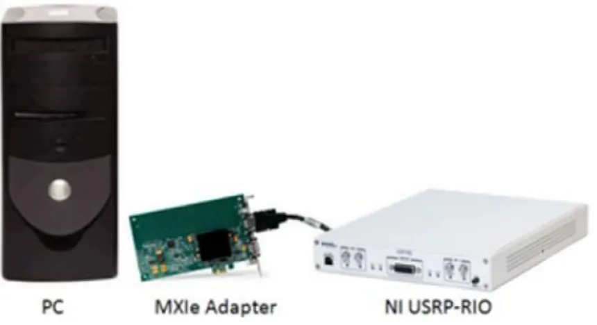
3.1.3.2 Multi-channel receiver: NI USRP-2955 ... 73
3.1.4 Antenna configurations ... 76
3.2 Low data traffic for PSL sensor ... 78
3.2.1 Acquisition campaign description ... 78
3.2.2 Relationship between data traffic conditions and performance ... 79
3.2.2.1 Accuracy of device-based AoA measurements ... 81
3.2.2.2 Accuracy of passive radar AoA measurements ... 85
3.2.3 Performance comparison of the two techniques ... 91
3.2.3.1 Passive Source Location performance ... 91
3.2.3.2 Passive Bistatic Radar performance ... 93
3.2.3.3 Techniques comparison and complementarity ... 95
3.3 High data traffic for PSL sensor ... 97
3.3.1 Acquisition campaign description ... 97
3.3.2 Performance comparison of the two techniques ... 98
3.3.2.1 Passive Source Location performance ... 98
3.3.2.2 Passive Bistatic Radar performance ... 100
3.3.2.3 Techniques comparison and complementarity ... 102
3.4 Summary ... 103
Chapter 4 Tracking techniques ... 106
4.1 Kalman Filter (KF) ... 106
4.2 Interacting Multiple Model (IMM) ... 107
Chapter 5 Interacting Multiple Model - Modified Innovation (IMM-MI) ... 110
5.1 Motion and Observation Models ... 111
5.2 Augmentation and Reduction ... 114
5.3 Sensor Fusion ... 115
5.4 State interaction ... 116
5.5 Filtering ... 117
5.6 Innovation Modification and Probability Update ... 118
5.6.1 Absence of PBR detections ... 120
5.6.2 Presence of PBR detections ... 121
7
Chapter 6 Tests on simulated target ... 123
6.1 Measurements generation ... 123
6.2 Setting of the employed methodologies ... 125
6.2.1 KF-NCV (Single Sensor) ... 125
6.2.2 KF-NCV (Sensor Fusion) ... 128
6.2.3 IMM (Single Sensor) ... 128
6.2.4 IMM (Sensor Fusion) ... 130
6.2.5 IMM-MI (Sensor Fusion) ... 131
6.3 Case study: Simulated Move-Stop-Move Target with changes of direction ... 132
6.4 Evaluation of the RMSE as a function of simulation time ... 133
6.5 Evaluation of the RMSE as a function of the Detection Probability for the PBR sensor ... 136
Chapter 7 Tests on experimental data ... 142
7.1.1 KF-NCV (Single Sensor) ... 146
7.1.2 KF-NCV (Sensor Fusion) ... 147
7.1.3 IMM (Single Sensor) ... 148
7.1.4 IMM (Sensor Fusion) ... 149
7.1.5 IMM-MI (Sensor Fusion) ... 151
7.1.6 Comparison of the analyzed methodologies in terms of positioning error ... 152
Chapter 8 Conclusion ... 155
BIBLIOGRAPHY ... 157
8
Chapter 1
Introduction
1.1 Background and State of the Art
In the recent years, great effort has been devoted to the localization of human targets and small objects in local area environments. The interest on this topic is motivated by the huge amount of possible applications that require the knowledge of the target position:
- for monitoring and surveillance applications in critical areas, such as ports or airports;
- as support in rescue missions inside buildings (for example in case of fire), where the capability of quickly and accurately coordinating the components of rescue teams is a key element for the success of the rescue operation, as discussed in [1];
- in medical applications focused on the improvement of quality of life for disabled people (for example, in [2] an application for blind persons is supposed, while in [3] an extensive review is performed on the use of Radio Frequency (RF) sensing for healthcare applications);
- in the offer of different kind of services (for museums, shops, hospital and universities).
In outdoor environments, this operation is obtained through the exploitation of satellite signals, using global navigation satellite systems as GPS, Glonass or Galileo. As well known, these signals have strong limitations indoor and require targets to cooperate in order for them to be detected and localized. For this reason, an alternative solution is to employ other RF signals already available, for localization aims. They have a wide coverage also in indoor areas and can be used to detect and localize non-cooperative targets. Depending on the requirements of the specific application, several waveforms can be exploited as, for example, FM [4]-[6], DVB-T [7]-[12] and Wi-Fi signals [13]-[20].
Different approaches can be considered to perform localization when exploiting these signals. In particular, these strategies can be discriminated based on whether an active device carried by the human target is required or not, and on the level of cooperation of the specific target. Obviously, all the classes of localization techniques have inherent advantages and drawbacks. A recent comprehensive review of such techniques is presented in [21], which compares the relative merits and issues, while a review of the only device-free localization strategies is reported in [22].
In particular, the expansion of the Fi networks in urban environments has led to the employment of Wi-Fi signals in several applications, thanks to the coverage that they offer in both indoor and outdoor environments. It is clear that this characteristic makes them especially suitable for short range localization and surveillance applications [16], as well as for extracting target characteristics as cross-range profiles, [23].
9
Based on the aforementioned classification of the localization techniques, a brief description of the main strategies for each class is now presented.
Cooperative localization
When the target voluntarily tries to be localized, we refer to cooperative localization. Several studies can be found in the technical literature, related to this case; one of the most used techniques is fingerprinting. It is of great interest the exploitation of Wi-Fi signals, when this strategy is used.
In many cases, the Received Signal Strength (RSS) is measured at different locations of the considered environment. The prints obtained in this way are stored into a dataset (offline measurements or ‘calibration stage’), and are used as a benchmark to evaluate target position (online measurements or ‘localization stage’). This stage is performed applying different strategies, e.g. K-Nearest Neighbor (K-NN), Support Vector Machine (SVM), etc. which are the preferred ones in this kind of studies.
Moreover, fingerprinting is not only defined based on signal strength, but also based on channel impulse response, [24]. This strategy leads to better performance, and it is particularly suitable to be applied when channel response can be easily inferred.
In other studies, use of Radio-Frequency Identification (RFID) technology has been proposed. This technology is often used in positioning systems where active cooperation from the user that needs to be localized can be exploited (as already mentioned in the example of rescue teams coordination, described in [1]). One of the main drawbacks of RFID technology is the need of a dedicated infrastructure, thus resulting in increased deployment costs.
All these strategies lead to good localization results (mainly with the application of advanced probabilistic methods), if particular conditions occur. Specifically, due to the need of active cooperation from the target, these strategies cannot be applied whether the object/person to be localized does not carry a mobile device or the Wi-Fi connection is disables. Moreover, obtainable accuracy strongly depends on actual operating conditions.
Partially cooperative localization
When the target provides involuntary contribution to positioning, we refer to partially cooperative localization. The target can be defined as system user, since it carries an active device and its transmissions are exploited. It is a non-cooperative localization, but the target, by carrying a device, provides a contribution to the definition of its position. We refer, in this case, to passive positioning: user does nothing to be voluntarily located, but localization occurs just as a consequence of carrying an emitting device. Even in this case Wi-Fi signals can be exploited, as the communications between Access Point (AP) and device when they are connected.
Specifically, detection of packets transmitted from the target (object/person) under exam is performed through multiple receiving antennas (typically 3 of 4, depending on the desired measurements and on the
10
capabilities provided by the receiving platform). Data collected by the antennas are processed by means of proper techniques to obtain an estimate of user position.
The techniques mainly used are Time of Arrival (ToA) estimation, Angle of Arrival (AoA) estimation and Time Difference of Arrival (TDoA) estimation.
These techniques allow the determination of the position of user carrying the mobile device; specifically, estimation is more reliable the more the target is stationary, since in this case an increased number of packets is available to perform the estimation. It would therefore be interesting evaluating the relationship between estimation reliability and number of available packets.
They are potentially characterized by low accuracy in position estimation, mainly in indoor scenarios, due to the difficulty in defining the propagation model for signals in complex environments (multipath, etc.). Nevertheless, different studies have been carried out aiming at removing this kind of problem, in most cases by jointly using AoA and ToA estimations, [25].
Main contributions in this area are related to scenarios with user voluntarily cooperating to be located, so great effort is requested with respect to the possibility to exploit only the communications occurring during usual Wi-Fi connection activities.
Non-cooperative localization
Finally, if there is no collaboration from the target, neither voluntary nor involuntary, and it is detected only due to its interaction with signals present in the environment, we refer to non-cooperative localization.
In this framework, interesting studies have been carried out by University of Utah, by exploiting Radio Tomographic Imaging (RTI) technique to localize a person not carrying a mobile device (this is the reason why this methodology is usually referred in technical literature as ‘device-free localization’). As described in [26], RTI is based on the principles of two different systems for the realization of images: radar systems and computed tomography, used for medical applications.
Another method to perform non-cooperative localization foresees the use of passive radars exploiting Wi-Fi signals as waveforms of opportunity. This topic has been widely addressed by our research group in the DIET Department at Sapienza University of Rome. The developed WiFi-based passive radar demonstrator performs the localization and tracking of moving targets, there including vehicles and human targets. Some interesting studies in this field are described in [14]-[17],[23] and [27].
1.2 Research challenges and selected approach
The localization of human targets and small objects in local area environments is one of the most attractive issues of the last years. As explained before, each strategy is characterized by inherent advantages and drawbacks. In particular, in some cases the main problem is the impossibility for the single technique to detect and localize a target in particular conditions. To face this problem, we decided to propose the joint use of different positioning techniques.
11
In addition to the achievement of important improvements in positioning accuracy, we are also interested in performing the localization for the entire observation time where the target stays in the area of interest.
To do that, two different techniques based on Wi-Fi signals have been considered in this work: firstly, the Passive Bistatic Radar (PBR) that exploits the AP as illuminator of opportunity is an interesting solution, especially for surveillance applications in local area environments, because it provides the position of non-cooperative targets, which do not carry an active device (the so called “device-free localization”), [17]. Secondly, supposing that the target has the possibility to transmit Wi-Fi signals (use of mobile devices for a human target), the Passive Source Location (PSL) that in contrast uses the device transmissions to define the position of the target, is another possible strategy to reach the same goal, [21]. Their concept is depicted in Figure 1.1.
As well known, the passive radar is very effective in detecting moving targets by using clutter cancellers. The extraction of stationary targets echoes is generally more complex and less effective, due to the background echoes cancellation stage performed during the processing. Moreover, due to the frequency bandwidth of the Wi-Fi waveforms, spanning from 11 to 20 MHz, the range resolution is not better than a few meters, which makes it difficult to discriminate closely spaced persons. In contrast, good Doppler frequency resolution is available, which provides good localization performance when the target is well separated in Doppler from the other targets and even allows to obtain cross-range profiles, [23].
As explained before, the use of Wi-Fi signals allows also exploiting the waveforms emitted directly by the device to localize them, [21].
The autonomous RF emissions of devices that attempt to connect to the Wi-Fi network allow us a different way to localize the human targets. As mentioned also in [21], to reach this purpose, many techniques have been investigated and applied. Largely used are position solutions based on the estimation of AoA, ToA and TDoA. As apparent, this only allows localizing human targets carrying an active Wi-Fi device. In addition, it could be potentially inaccurate for moving targets. On the other hand, it is an interesting solution for stationary targets localization and it allows the unambiguous association of the transmission to a specific target, based on the device MAC address, so that even very closely spaced persons can be discriminated.
Figure 1.1. Sketch of WiFi-based PBR and PSL approaches. Transmitted signal Device transmission Received echo TX (AP) RX RX
12
Our purpose is to compare the relative performance of this two localization techniques based on the IEEE 802.11 Standard, [28], and to verify their complementarity, aiming at their joint exploitation in a unified system, which exploits at the best the features of both the employed sensors.
Through the years, great interest is also devoted to the target tracking. This topic has still several open issues. In particular, one of the most interesting problems is the tracking of move-stop-move targets. In fact, despite the low complexity of the single motions, its management is very hard in practical applications. First of all, the detection of stationary targets is still a problem when the passive radar is exploited. Secondly, the similarity between the two types of motion could generate important ambiguities when particular techniques are employed.
The aforementioned problems increase when the examined target frequently and rapidly changes its motion status. This is the case, for example, of the smallest targets which can be found in local area environments, as persons or drones. In this case, the Kalman Filter (KF) and the classical Interacting Multiple Model (IMM) are not effective to reach this purpose.
In order to find a solution to this problem, in this thesis two novelties in common tracking strategies have been introduced:
1) Data Fusion techniques are applied in order to exploit the advantages of the two employed sensors and extend the time in which the examined target is localized.
2) A modified version of the IMM, that we called Interacting Multiple Model - Modified Innovation (IMM-MI) is devised with the purpose of compensating for the limitation of the existing techniques. Even this time the knowledge of the characteristics of the single sensors is exploited, in order to help the decision on the motion model that has to be used.
The research approach followed in this thesis to obtain these results is represented in Figure 1.2.
13
The first step is the characterization of the two sensors. In this phase, we focused on the analysis of the measurements that the specific sensor can exploit to estimate the target position and the derivation of the related positioning techniques. In particular, since the PBR has been extensively studied by our research group, greater attention was devoted to the characterization of the device-based sensor, for which innovative techniques for the estimation of the TDoA are also presented.
After the sensor descriptions, their performance is analyzed and compared. The inherent features of the two strategies and the results obtained from their comparison on experimental data have shown an interesting complementarity between them. This result opens the way to the development of appropriate sensor fusion techniques, which characterizes the final part of this thesis. The proposed strategy is then evaluated on both simulated and experimental data on a move-stop-move target, and its performance is compared with existing techniques (KF and IMM). Even the employment of sensor fusion techniques on classical tracker is tested. The results show that the use of more sensors provide better performance with respect to the use of single sensor versions. However, some problems still appear when the target changes its motion. The IMM-MI is a possible solution to these problems. In fact, it outperforms the other strategies, since it provides the best performance in terms of positioning accuracy, target motion recognition capability and percentage of acquisition time covered by this strategy.
1.3 Outline of the Thesis
With reference to the scheme presented in Figure 1.2 this thesis has been organized as follows.
Chapter 2. The two PBR and PSL sensors and the related localization strategies are described in detail. For
each sensor, the analysis has been divided in three main parts. Firstly, different techniques for the measurement extraction have been studied. In particular, a deepened analysis has been carried out for the TDoA estimation, for which innovative techniques are also proposed. Secondly, based on the measures studied in the first part of this Chapter, the relative positioning strategies are derived and compared in terms of localization accuracies. Finally, the processing schemes of the two sensors are presented and the main blocks are described.
Since the PBR has been extensively analyzed by our research group in the past, in Chapter 2 the main features of the passive radar are briefly summarized, giving more importance to the enhancement with respect to the previous system, while larger space has been dedicated to the PSL description.
Chapter 3. As the deepened knowledge of the two sensors is now available, the performance of the PBR
and PSL sensors in terms of localization accuracy is faced in this Chapter. In particular, the relationship between data traffic conditions and performance for the two strategies, and their performance comparison are evaluated on experimental data. Specifically, the comparison of the two localization strategies has been performed on two different data sets characterized by different network conditions.
14
Chapter 4. After the target localization, the tracking stage can be applied in order to improve the positioning
performance. Therefore, the main existing tracking algorithms, namely the KF and the IMM, are briefly presented, and the relative advantages and limitations are recalled.
Chapter 5. A new methodology for target tracking is proposed, which exploits the inherent differences
between the PSL and the PBR sensors, in order to develop a consistent and effective method for small target localization and tracking, especially for move-stop-move targets. The proposed strategy uses a modified version of the IMM approach together with Data Fusion techniques, that take into account the differences between the measurement’s accuracies of the employed sensors. In the modified version of the IMM method, the information related to the presence or absence of the PBR estimates is used to help the choice between the employed filters, through the modification of the Innovation.
Chapter 6. The proposed strategy is then compared with the KF and the IMM methods over a simulated
target. Specifically, the stop & go motion has been simulated, aiming at showing the capability of the proposed strategy to follow the target behavior, thanks to the possibility to exploit the knowledge of the characteristic of the employed sensors. In this analysis, for the KF and the IMM, both the single sensor and the sensor fusion versions are considered, in order to highlight the advantages of the joint use of two different sensors. Two analysis have been performed: 1) the evaluation of the Root Mean Square Error (RMSE) as a function of the simulation time, and 2) the evaluation of the RMSE as a function of the Detection Probability for the Passive Radar.
Chapter 7. The evaluation of the performance for the aforementioned techniques has finally been carried
out on experimental data, through the design of appropriate acquisition campaigns.
15
Chapter 2
Sensors description
Before starting with the detailed description of the two proposed sensors, it is convenient to briefly describe the main characteristics of the employed Wi-Fi signals.
2.1 IEEE 802.11 Standard and WiFi packets features
The IEEE 802.11 Standard, [28], defines the main characteristics of Wireless Local Area Networks (WLANs). It presents one Medium Access Control (MAC) and several Physical (PHY) layer specifications. In the last years, different versions of this standard have been developed. In particular, the IEEE 802.11a Standard uses the 5 GHz band, while 802.11b/g/n operate in the 2.4 GHz band. Different data rates can be used, thanks to the employment of different modulation and coding schemes.
In the 2.4 GHz band the spectrum is divided into 14 channels, spaced 5 MHz each other. Due to the Wi-Fi bandwidth, spanning from 11 to 20 MHz (or higher values in some cases), depending on the specific Standard version or modulation type, it is evident that the Wi-Fi channels are partially overlapped and so it is possible to have interference among transmissions occurred in consecutive channels. Moreover, multiple users can share the same channel, therefore they have to alternate the medium occupation (TDMA approach) in order to avoid contemporary transmissions. To reduce the risk of collisions, the Carrier Sense Multiple Access with Collision Avoidance (CDMA/CA) access mechanism is adopted.
As well known, the Wi-Fi communications use the packet switching approach to exchange information. The function of a specific packet is defined by the type/subtype field. There are three different packet types (management, control and data), and several subtypes for each of them, e.g. beacon, association request, authentication, etc.
To establish the connection between APs and devices, which is the primary operation before any communication activity, management packets are transmitted. There are two ways to perform the searching of stations in a given area: the passive and the active scanning techniques. In the first case, the AP periodically sends beacons in broadcast mode to announce its presence. The transmission rate and the operating channel are set previously. The latter foresee that a mobile station sends probe requests in broadcast mode on a single channel and waits for answers from the APs in proximity. If it does not receive any probe response, it switches to another channel and it repeats the same operation.
After that, the mobile station sends the authentication frame to the desired AP, after the reception of the AP answer, it transmits the association request and, when the association stage is completed, the data transfer
16
between AP and device can start. Even very short communications are therefore characterized by the exchange of many packets of different types, which have different features and frame formats. It is also important to notice that the packet length varies according to its subtype. This is related to the differences among the frame formats of different packets. In addition, it also depends on the dimension of the payload in data packets.
These considerations confirm that the exploitation of the huge amount of Wi-Fi signals exchanged during common connection or communication activities represents an attractive solution for localization applications.
2.2 Passive Bistatic Radar (PBR)
The Passive Radar is one of the most attractive solution for the localization of different types of target. It works as a common radar, but its main feature is the bistatic form. In fact, the Passive Radar exploits the signals emitted by transmitters of opportunity, namely it does not use its own waveform, but pre-existent transmissions devised for other communication purposes. This means that receiver and transmitter are located in different places.
Among the advantages of this technique, we can mention the low costs of realization and maintenance (due to the lack of the transmitter), the possibility to avoid electromagnetic disturbances, the low impact on the environment, and so on. On the other hand, the impossibility to properly design and control the transmitted waveform makes the processing much more complicated (reference reconstruction, etc.) and the performance can decrease if proper techniques are not employed.
In particular, as explained in the Introduction, for short-range applications Wi-Fi signals are particularly suitable, thanks to the coverage that they have reached in recent years in local area environments. For this reason, in this thesis we focus on this typology of signals. The specific transmitter of opportunity is the Access Point, whose signals emitted for communication purposes in this case are used for the localization of human targets and small objects. As explained above, the Wi-Fi Standard established that the information is not transmitted with a continuous wave, but it is divided in packets. This means that a pulsed shape characterizes the transmissions exploited by the PBR. Following this consideration, in this work the terms pulse and packet are used as synonyms. In particular, the specific packets (beacons) that the AP periodically sends in broadcast mode to announce its presence in a specific area, represent an interesting choice for the design of the described passive radar: the possibility to exploit a constant Pulse Repetition Time (PRT), due to the definition of a constant Beacon Interval (BI), which is defined as the time spacing between consecutive beacons, encourages the use of these signals. Typical beacon transmissions are shown in Figure 2.1.
17
In the next sections, the main parameters measurable by the Passive Radar are presented together with their combination to perform the positioning in the XY-plane.
2.2.1 Measurement extraction
The PBR sensor can provide different measurements. Each measure is estimated on the specific target detection, namely after the applications of all the operations summarized in the processing scheme that will be described in detail in Section 2.2.3.
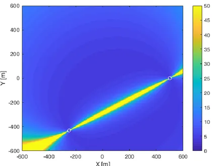
A single surveillance antenna can estimate both the bistatic range and the bistatic Doppler frequency (which is directly connected to the bistatic velocity) of a target. With a couple of closely spaced antennas, it is possible to estimate even the Angle of Arrival (AoA) of the received target echo. A sketch of the considered geometry with the relevant parameters in shown in Figure 2.2, where the line defined by the AoA, and the ellipse defined by the bistatic range are displayed.
Figure 2.1. Example of a sequence of Wi-Fi packets.
18
Specifically, the bistatic velocity of the target is obtained from the Doppler frequency, 𝑓𝐷, measured on the
received target echo. As it is well known, the relationship between Doppler frequency and velocity is the following
where 𝜆 is the wavelength related to the Wi-Fi channel where the transmitter, in our case the Access Point, is transmitting.
The bistatic range is defined as the sum of two contributions: i) the distance between transmitter (AP) and target and ii) the distance between target and receiver
where 𝑅𝑇𝑋,𝑡𝑎𝑟𝑔𝑒𝑡 and 𝑅𝑡𝑎𝑟𝑔𝑒𝑡,𝑅𝑋 are the two contributions described above.
Therefore, we obtain
where (𝑥𝑇𝑋, 𝑦𝑇𝑋) are the coordinates of the transmitter, (𝑥𝑅𝑋, 𝑦𝑅𝑋) are the coordinates of the receiver, while
(𝑥𝑢, 𝑦𝑢) are the coordinates of the target, which have to be estimated.
In particular, the bistatic range is directly connected to time of arrival, 𝜏, through the following relation
where 𝑐 is the speed of light.
Combining the equations (2.3) and (2.4), we obtain
As it is clear from (2.5), in this way we have only one equation in two unknowns (𝑥𝑢 and 𝑦𝑢).
For the localization in the XY-plane, it is therefore necessary to add a further equation that is provided by the employment of an additional receiver.
As mentioned above, if the second receiver is very close to the first one, it is possible to estimate also the AoA, 𝜃̂. As shown in Figure 2.3, this angle is linked to the phase difference between the signals received by the two surveillance antennas, 𝛥𝜑̂ , through the relation
where 𝜆 represents the wavelength related to the Wi-Fi channel on which the device is transmitting, while 𝑑 is the distance between the antenna elements, as defined above.
𝑣𝑏𝑖𝑠 = 𝑓𝐷· 𝜆 (2.1) 𝑅𝑏𝑖𝑠 = 𝑅𝑇𝑋,𝑡𝑎𝑟𝑔𝑒𝑡+ 𝑅𝑡𝑎𝑟𝑔𝑒𝑡,𝑅𝑋 (2.2) 𝑅𝑏𝑖𝑠= √(x𝑇𝑋− xu)2+ (y𝑇𝑋− yu)2+ √(x𝑅𝑋− xu)2+ (y𝑅𝑋− yu)2 (2.3) 𝑅𝑏𝑖𝑠 = 𝑐 · 𝜏 (2.4) √(x𝑇𝑋− xu)2+ (y𝑇𝑋− yu)2+ √(x𝑅𝑋− xu)2+ (y𝑅𝑋− yu)2= 𝑐 · 𝜏 (2.5) 𝛥𝜑̂ =2𝜋𝑑 𝜆 sin 𝜃̂ (2.6)
19 From (2.6), it can be easily derived
All parameters in the equation (2.7) are known, except for the phase difference which, instead, has to be estimated from the received target echoes. In this case, the following expression applies
where 𝑥1 and 𝑥2 are the samples in the bi-dimensional Cross-Correlation Functions (2D-CCF) corresponding
to the location of the specific target detection, for the two receivers exploited for the angle estimation.
2.2.2 Positioning techniques
After the definition of the measures that can be used for the PBR sensor, it is important to have an idea of the possible strategies to obtain the target localization in the XY plane.
The positioning can be performed in different ways, also depending on the number of receiving nodes available and the number of antennas contained in each node.
As explained in the previous section, for the Passive Bistatic Radar, the bistatic range and the angle of arrival can be exploited for the target localization.
The considered combinations of bistatic range and AoA for target localization are summarized in Table 1. 𝜃̂ = 𝑎𝑟𝑐𝑠𝑖𝑛 (𝜆 ⋅ 𝛥𝜑̂
2𝜋𝑑 ) (2.7)
𝛥𝜑̂ = arg (𝑥2 𝑥1
) (2.8)
20
Table 1. Measurement combinations for target localization with the PBR sensor.
Number of nodes PBR sensor
1 Receiving Node (2 Antennas) 1 Range + 1 AoA 2 Receiving Nodes (max 4 Antennas) 2 Ranges 1 AoA + 2 Ranges
In this table, when two measures of angle are used, four surveillance antennas are employed to acquire the echoes scattered by the target.
The positioning techniques for the PBR sensor are extensively discussed in [17]. In particular, the treatment is divided into two blocks:
1) The target localization using the minimum number of measures. 2) The target localization using multiple measurements.
The following combinations were analyzed for the first case.
A) Two bistatic range measurements provided by two receiving nodes after the detection stage.
B) Two bistatic range measurements obtained from two receiving nodes after a range/Doppler tracking stage.
C) A range measurement and an AoA measurement provided by a single receiving node.
Instead, for the second case, two bistatic range measurements and one AoA measurement estimated by two nodes were exploited. Each of the three measurements defined a specific equation where the unknowns were the coordinates of the target in the XY-plane, i.e. (𝑥𝑢, 𝑦𝑢). This means that the system was overdetermined,
therefore the Least Square (LS) solution and the Maximum Likelihood (ML) solution were used for the 2D localization of the target.
In the following, we briefly summarize the main results reported in [17], where this study has been extensively discussed.
The system of equations when two measurements of range and one of AoA are exploited is the following
where (𝑥𝑇𝑋, 𝑦𝑇𝑋) are the coordinates of the transmitter, (𝑥𝑅𝑋, 𝑦𝑅𝑋) are the coordinates of the receiver, (𝑥𝑢, 𝑦𝑢)
are the coordinates of the target, which have to be estimated, 𝑅̂𝑏𝑖𝑠1 and 𝑅̂𝑏𝑖𝑠2 are the bistatic ranges measured
{ 𝑅̂𝑏𝑖𝑠1= √(x𝑇𝑋− xu)2+ (y𝑇𝑋− yu)2+ √(x𝑅𝑋1− xu) 2 + (y𝑅𝑋1− yu) 2 𝑅̂𝑏𝑖𝑠2= √(x𝑇𝑋− xu)2+ (y𝑇𝑋− yu)2+ √(x𝑅𝑋2− xu) 2 + (y𝑅𝑋2− yu) 2 𝜃̂ = tan−1(xu yu ) (2.9)
21
by the two nodes, while 𝜃̂ is the angle of arrival estimated by the receiver containing two closely spaced antennas.
The LS solution of the system in (2.9) is
where 𝐮 is the vector containing the target coordinates, 𝐮0 is the target tentative position used for the
first-order Taylor series approximation, 𝐇 is the matrix of the direction cosines, 𝐦 is the representation with the matrix notation of the known terms 𝑅̂𝑏𝑖𝑠1, 𝑅̂𝑏𝑖𝑠2 and 𝜃̂, namely
and 𝐦0 is its expression calculated in 𝐮0.
The corresponding positioning error over the XY-plane is given by
where 𝚺𝐌 indicates the covariance matrix of the measurement errors defined as
and 𝜎𝑅21, 𝜎𝑅22 and 𝜎𝜃2 are the variances of the errors on 𝑅𝑏𝑖𝑠1, 𝑅𝑏𝑖𝑠2 and𝜃, respectively.
For the ML solution, the target position can be expressed as
The results reported in [17] have shown that the ML produced better results with respect to LS approach, since the ML provides the possibility to weigh the measurements according to their accuracy, therefore it relies mainly on the angular information.
The comparison of all the methodologies has shown that the localization can be performed by using only range measurements, but before the localization a tracking stage in the bistatic range/Doppler plane has to be applied. In addition, it has been demonstrated that the use of the angular information provides an improvement in performance.
According to the aforementioned results, in the next analysis we will use one bistatic range measurement and one AoA measurement to perform the target localization in the XY-plane. This choice allows i) increasing the achievable positioning accuracy with respect to the use of only range measurements, thanks to the exploitation of an additional measurement of AoA, and ii) reducing the processing time avoiding the employment of iterative methods. 𝐮 = (𝐇T𝐇)−1𝐇T(𝐦 − 𝐦 0) + 𝐮0 (2.10) 𝐦 = [𝑅̂𝑏𝑖𝑠1 𝑅̂𝑏𝑖𝑠2 𝜃̂] 𝑇 (2.11)
𝚺
𝒖𝐿𝑆= (𝐇
T𝐇)−1𝐇T𝚺 𝐌H(HTH)−1 (2.12)𝚺
𝑴= [
𝜎
𝑅210
0
0
𝜎
𝑅220
0
0
𝜎
𝜃2]
(2.13) 𝐮 = (𝐇T𝚺𝐌−1𝐇) −1 𝐇T𝚺𝐌−1(𝐦 − 𝐦0) + 𝐮0 (2.14)22
2.2.3 Processing scheme
The passive radar demonstrator developed at Sapienza University of Rome ([16]-[17]) has been applied. The generic processing scheme is sketched in Figure 2.4.
After the acquisition of the Wi-Fi signals through the available surveillance antennas, the first step is the packet extraction and their subsequent identification based on the source MAC address written in each packet. In this way the signals emitted by the AP can be discriminated and used as transmissions of opportunity for the Passive Radar.
The processing scheme presented in Figure 2.4 is the most generic representation when a quad-channels receiver is employed. However, a basic distinction can be made with respect to the number of channels actually dedicated to the acquisition of surveillance signals.
In particular, we are interested in considering two different situations, namely 1) The exploitation of the minimum number of receiving channels; 2) The exploitation of all the four receiving channels.
With reference to the first point, we can exploit three receiving channels for the acquisition of the signals of interest. In particular, two channels are occupied by the two surveillance antennas, while the third one can be dedicated to the acquisition of a clean copy of the reference signal, directly extracted by the Access Point. This choice provides the advantage to know exactly the signals emitted by the transmitter of opportunity, producing an improvement in performance. For this reason, the Reference reconstruction block in Figure 2.4 can be discarded and the subsequent operation can be performed exploiting the real reference signal.
For the second case, all the receiving channels are connected to the surveillance antennas. This provides on one hand the possibility to exploit more information, through the estimation of additional measurements (for example two AoA measurements) but, on the other hand, it disables the reference signal acquisition. This means
23
that such signal must be reconstructed with further post-processing operations, since this is necessary to perform the target localization with the passive radar system.
After these preliminary steps, the processing continues with the evaluation of the 2D-CCF, obtained by cross-correlating the surveillance signals with the reference signal (real or reconstructed) on a pulse by pulse basis. Thereafter, the obtained results are coherently integrated over a set of consecutive pulses. This requires to be repeated for all Doppler frequencies of interest, thus providing the 2D output as a function of both bistatic range and bistatic Doppler frequency.
As shown in [29], the Ambiguity Function (AF) of the Wi-Fi signals is characterized by high sidelobes in both range and Doppler dimensions. Therefore, proper techniques for the Range and Doppler sidelobes control are applied. In particular, the knowledge of the modulation of the beacons periodically transmitted by the AP (DSSS) allowed to devise suitable weighting networks. For the range sidelobes control, the two weighting networks proposed in [30] are used. The first one is called Barker Weighting Network (BWN) and is necessary to reduce the sidelobes within time delays of 1μs that are due to the 11-chip Barker code which characterized this signal. The second one is used to control the sidelobes due to the cyclical repetition of the Barker code. The doppler sidelobes reduction has been devised in [31] and uses well-known linear programming algorithms.
The processing scheme includes the clutter/multipath cancellation stage for the disturbance removal. In particular, the Sliding Extensive Cancellation Algorithm (ECA-S) is used, [32].
After that, the range/Doppler maps are evaluated and the CFAR threshold is applied; when the two-out-of-two criterion is exploited, target detection is declared only for the targets that exceed the threshold on both the receiving channels. Thereafter, the tracking of the detected targets is performed on the Range/Doppler plane. As demonstrated in [17], this tracking stage increases the positioning accuracy when the localization in the XY-plane is performed.
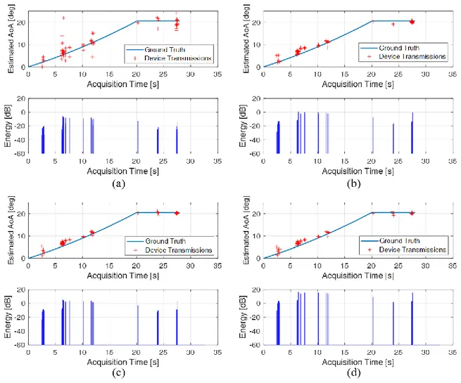
For the plots of the selected tracks, both the filtered bistatic range and the angle of arrival are estimated.
2.3 Passive Source Location (PSL)
The PSL sensor can estimate the target position through the combination of Time Difference of Arrival (TDoA) and AoA measurements. Specifically, the localization can be performed by exploiting only AoA measurements, only TDoA measurements or their combination. In Figure 2.5, a sketch of the above-mentioned measurements is shown with reference to a typical geometry with two receiving nodes. In the case shown in Figure 2.5(a), only three antennas are necessary to perform the target localization in the XY-plane, while when two measurements of AoA are considered, each node needs at least two antennas, as displayed in Figure 2.5(b).
24
2.3.1 Measurement extraction
2.3.1.1 Techniques for Time Difference of Arrival (TDoA) estimation
The TDoA between two signals received by two different surveillance antennas provides a measurement related to the target position. In particular, it defines the hyperbola on which the target is located.
As mentioned above, to achieve a more accurate localization of a target, it is necessary to choose conveniently the technique for TDoA estimation that yields better performance in terms of positioning accuracy and processing time. To this purpose, different strategies have been investigated.
Before starting to describe the approach followed for this study and the proposed techniques, it is necessary to introduce the main strategies that can be applied when the TDoA measure has to be estimated. There are two ways to define the TDoA, through the exploitation of two separated antennas:
• By neglecting the typology of the signal;
• By exploiting the a priori knowledge of the signal available, namely its modulation format (we will use the Wi-Fi emissions of the target (mobile device or drone), that can be modulated in different ways defined into the IEEE 802.11 standard, [28]).
In the first case, we would use the data received by two antennas, made available to a “Master” sensor (e.g. ‘RX2/3’ node in Figure 2.5(a)) that will be able to realize the operations necessary for the TDoA estimation on the two received signals. As apparent, this implies the need to transfer data at the original data rate, from a sensor (e.g. ‘RX1’ node in Figure 2.5(a)) to the “Master” sensor, therefore a dedicated infrastructure must be realized.
In contrast, in the second case, the a priori knowledge of the modulation format of the received signal allows the exploitation of its known parts (usually the preamble) for the comparison of the signal received by the
(a) (b)
25
antenna and a clean copy of this known portion of signal, pre-recorded in the receiving nodes. In this way, each receiving node estimates the delay of the signal in input with respect to the reference one (Time of Arrival) and then transmits only the estimated value, and the difference of these values (TDoA) can be defined later.
As mentioned above, both these strategies have inherent advantages and drawbacks. Firstly, the second approach is interesting because it provides the possibility to avoid the transfer of the entire signal to obtain the estimation of the measure of interest; in addition, the reduction of the used packets dimensions (limitation to a shorter portion of the signal containing the preamble) allows to reduce the elaboration time but, on the other hand, it could introduce a deterioration of the estimation accuracy, due to the exploitation of less samples. However, this strategy needs additional pre-processing operations, which provide the information about the typology of the received signal, in order to compare it with the correct preamble associated to that specific standard.
In this first part of the study, we decided to totally free ourselves from the necessity to know the characteristics of the received signals (if we exclude the information of the bandwidth and the carrier frequency), and so we examine in depth the first strategy, but it is important to highlight that the same techniques can be extended also to the other case.
In particular, the analysis has been performed on real data, namely signals actually transmitted by a Wi-Fi transmitter, but in favorable conditions, that is:
• The estimation is performed on the Reference signal, namely the packets directly acquired from the Access Point (AP), therefore the signal is clean (high Signal-to-Noise Ratio, SNR).
• A fixed length (1500 samples) is considered for the employed packets.
• We deliberately inject white Gaussian noise to the Reference signal to degrade the SNR, in order to emulate the signal received by the antennas.
• In order to simulate the signal received by the second surveillance antenna, the Reference signal is duplicated and additive noise is injected even to it; a delay of a fraction of sample is generated and applied to this Reference copy, so that a cleaner performance evaluation can be obtained.
• It is important to understand that the noise realizations applied to the two “surveillance” signals are independent one another and they are generated with respect to a specific noise power, defined by the desired SNR. In particular, we analyze 9 different values of SNR (from -5 dBs to 35 dBs, with steps of 5 dBs).
Different strategies have been proposed in literature, [33]-[40]. In the following Sections, the considered techniques for TDoA estimation are described. The basic idea is briefly explained and the principal formulas are derived. In addition, we present the evaluation of the performance in terms of accuracy. The whole discussion is faced taking also into account the possibility to reduce the elaboration time.
26
2.3.1.1.1 Cross-Correlation and Oversampling Method (CCF-OVS)
The first technique that we analyze exploits the simple cross-correlation between the signals of which we want to evaluate the time difference of arrival. Without further modifications, this strategy allows to estimate the TDoA with a resolution defined by the sampling time, and so fractional delay cannot be estimated. To do that, it is therefore necessary to oversample the curve obtained through the cross-correlation operation, by using an oversampling factor that allows to reach the desired resolution.
The main steps of this method are the following:
1) Calculation of the Cross-Correlation (over single packets) between the signals received by the two antennas, that is 𝑅𝑠1𝑠2(𝜏) = 1 𝑁∑ 𝑠1(𝑘𝑇) ∙ 𝑠2(𝑘𝑇 + 𝜏) 𝑁 𝑘=1 (2.15)
where T represents the sampling time, whereas 𝑠1 and 𝑠2 are the signals received by the two antennas.
2) Coarse estimation of the Cross-Correlation peak, through the following expression
3) Oversampling of a small portion of this correlation (10 samples) around its peak.
4) Determination of the time difference of arrival after oversampling (fine estimation), applying again the equation (2.16) on the new curve.
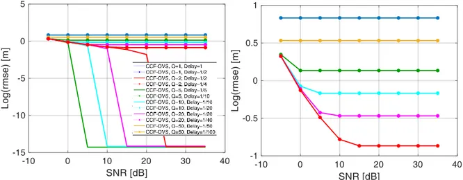
In Figure 2.6, the performance of the Cross-Correlation and Oversampling (CCF-OVS) method in terms of accuracy has been shown. In particular, we reported the Root Mean Square Error (RMSE) on the distance resulting from the TDoA estimation with respect to the Signal-to-Noise Ratio (SNR), for different oversampling factors.
For each oversampling factor, we have considered two different relative delays between the signals received by the surveillance antennas: the best case (solid line in the figure), when the delay corresponds to the new sample after oversampling (in fact, in this case, there are not errors due to the available resolution), and the worst case (indicated with stars in the same plot), that is when the delay is exactly in the mid-point of two consecutive samples of the signals (in this second case, the CCF-OVS method estimates a value of TDoA that corresponds to one of the two adjacent samples, defining an error equal to half sample of the oversampled signal). This behavior is evident in Figure 2.6 (where Q represents the oversampling factor, whereas Delay indicates the actual delay in samples between the two signals) and specifically by observing the limit value reached in the cases [Q=1, Delay=1/2] and [Q=2, Delay=1/4], that is exactly the distance related to half sample and 1/4 of sample, respectively, regardless the SNR. On the other hand, for the best cases (solid lines) the errors decrease rapidly to zero, even with low values of SNR.
𝛥𝜏̂ = argmax
27
In addition, it is possible to notice that, as expected, the performance increases when the oversampling factor increases.
In order to see in detail the behavior of the curves, we have reported in Figure 2.7 the same results shown in Figure 2.6, but in semilogarithmic scale. In particular, in the figure on the right we have reported only the worst cases.
This technique leads to good results, especially when higher oversampling factors are used, because they allow to reach higher accuracy. Nevertheless, even the computational cost increases when the oversampling factor increases, therefore it is necessary to find a tradeoff between these two components.
Alternatively, it is possible to study other strategies characterized by a lower computational cost.
Figure 2.6. Performance of the CCF-OVS method for different oversampling factors and delays.
28
2.3.1.1.2 Cross-Correlation and Fast Parabolic Interpolation Method (CCF-FPI)
A possible solution that allows to reduce the computational cost is the implementation of the Fast Parabolic Interpolation (FPI), as described in [33].
This technique is based on the assumption that the main lobe of the cross-correlation, containing the peak, can be approximated with a parabola; therefore, the research of the peak corresponding to the TDoA can be easily and accurately performed by searching the apex of this parabola, avoiding in this way the increasing of the elaboration time due to the oversampling operation (especially if a high factor is used) of the previous strategy.
In particular, the following steps are used:
1) Calculation of the Cross-Correlation (over single packet) between the signals received by the two surveillance antennas, as in (2.15).
2) Search of the peak of the Cross-Correlation (coarse estimation) through the formula (2.16).
3) Extraction of three samples around the peak, namely the sample related to the peak, the sample before it, and the sample after the peak
where 𝜏𝑃 is the instant related to the peak of the correlation, T is the sampling time and Q is the
oversampling factor.
4) Definition of the parabola passing for the three points
finding the coefficients a, b, c through the resolution of the system of equations consisting of the three parabolas determined by the points defined in (2.17), from which we obtain:
5) Calculation of the apex of the parabola (fine estimation) defined in (2.18), after having replaced the values in (2.19), (2.20) and (2.21), by using the known formula:
𝑥 = 𝑅𝑠1𝑠2(𝜏𝑃− 𝑇 𝑄), 𝑦 = 𝑅𝑠1𝑠2(𝜏𝑃+ 𝑇 𝑄), 𝑧 = 𝑅𝑠1𝑠2(𝜏𝑃) (2.17) 𝑔(𝜏) = 𝑎𝜏2+ 𝑏𝜏 + 𝑐 (2.18) 𝑎 =𝑥 + 𝑦 − 2𝑧 2 ∙ 𝑄2 𝑇2 (2.19) 𝑏 = −(𝑥 + 𝑦 − 2𝑧) ∙𝑄 2 𝑇2∙ 𝜏𝑃+ (𝑦 − 𝑥) 2 ∙ 𝑄 𝑇 (2.20) 𝑐 = 𝑧 +𝑥 + 𝑦 − 2𝑧 2 ∙ 𝑄2 𝑇2∙ 𝜏𝑃2− (𝑦 − 𝑥) 2 ∙ 𝑄 𝑇∙ 𝜏𝑃 (2.21)
29 𝛥𝜏̂ = − 𝑏
2𝑎 (2.22)
It is also possible, before point 3), to add an oversampling with a factor Q=2, that increase the estimation accuracy.
It is evident that the simple calculation of the numerical values necessary for the determination of the vertex of the parabola requires less elaboration efforts with respect to an oversampling characterized by a high Q.
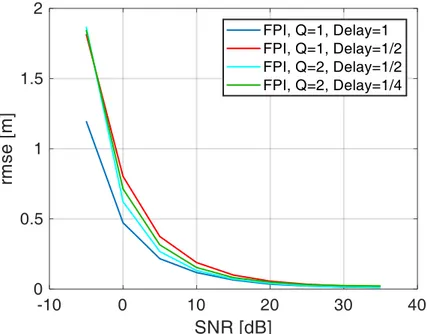
In Figure 2.8, we have reported the results obtained with the CCF-FPI method. We perform the same analysis carried out for the CCF-OVS method, namely the observation of the effect on the best and the worst cases for the delay, when a low oversampling (Q=2) is used or not (Q=1).
In this case, it can be noticed a general improvement of the performance in terms of estimation accuracy, as well as processing times.
2.3.1.1.3 Average Square Difference Function and FPI Method (ASDF-FPI)
In spite of performance improvement, the main problem for the processing times is determined by the calculation of the cross-correlation function.
Therefore, in [33], another type of strategy has been defined, with the purpose of avoiding the evaluation of the correlation. This methodology, instead of evaluating the product and sum which defines the cross-correlation, is based on the calculation of the sum of the differences of the values of the two signals. Therefore, replacing the product with the difference, even the computational cost should improve. This time it is the minimum of this function that has to be found, because it represents the point where the two signals are aligned, and so the TDoA to be found. After this operation, the FPI is applied also this time, in order to perform the “fine estimation” of the delay.
Figure 2.8. Performance of the CCF-FPI method for different oversampling factors and delays.
30 The main steps are the following:
1) Calculation of the Average Square Difference Function (ASDF), over single packet, between the signals received by the two surveillance antennas, that is
𝑅𝑠1𝑠2(𝜏) = 1 𝑁∑ |𝑠1(𝑘𝑇)−𝑠2(𝑘𝑇 + 𝜏)| 2 𝑁 𝑘=1 (2.23)
2) Search of the minimum of the ASDF of the signals (coarse estimation), as 𝛥𝜏̂ = argmin
𝛥𝜏 {𝑅𝑠1𝑠2} (2.24)
At this point, we can apply the steps and the formulas for the FPI. 3) Extraction of three samples around the minimum, (2.17).
4) Definition of the parabola passing through the three points, by the formulas (2.18), (2.19), (2.20) and (2.21).
5) Calculation of the apex of the parabola, (2.22).
Even this time, before the point 3), it is possible to add an oversampling with Q=2, that improve the estimation accuracy.
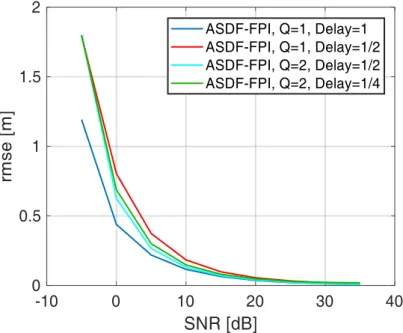
In Figure 2.9, we show the results for the ASDF-FPI method, for the same cases analyzed with the CCF-FPI method.
Figure 2.9. Performance of the ASDF-FPI method for different oversampling factors and delays.
31
It can be noticed that these results are comparable with those shown in Figure 2.8 for the CCF-FPI. In fact, the accuracy seams to depend principally on the way that is used to find the peak of the curve.
2.3.1.1.4 CCF + Slope-based Method
The slope-based method exploits the phase variation generated by a delay in the signal. In fact, a delay in time corresponds to a phase shift in frequency domain:
𝑥(𝑡 − 𝜏) → 𝑋(𝑓) ∙ 𝑒𝐹 −𝑗2𝜋𝑓𝜏 (2.25)
As apparent, this phase shift is linear in frequency and the line that describes its trend has slope equal to 2πτ. In particular, instead of estimating the ToA of each single signal through the comparison with a reference signal (as reported in literature, [34]-[35]), in this case it is directly estimated the Time Difference of Arrival (TDoA) between two surveillance signals. Moreover, in contrast to the strategies adopted in [34] and [35], in our approach the features of the OFDM signal were not directly exploited; in this way, these techniques can be applied over a generic signal, regardless the modulation format. In detail, the strategy to obtain this measurement is based on the estimation of the ratio of the spectra of the received signals (or equivalently, on the product of a spectrum and the complex conjugate of the other one), whose phase is represented by the difference of the phases of the two signals. As can be easily understood from (2.25), the slope of this new phase is linked to the relative delay between the two signals, namely 𝛥𝜏, which represents the TDoA we are looking for, thanks to the equation
𝛥𝜏 = − 𝛥𝛷
2𝜋 ∙ 𝛥𝑓 (2.26)
where the “slope” is 𝛥𝛷/𝛥𝑓 (or -2π𝛥𝜏, as explained before).
This method has been applied on both OFDM and DSSS signals. In the first case, simulated signals have been used. These signals have been generated by a generator of Wi-Fi “HT Format” signals, which uses OFDM modulation. In the second case, real data have been used. In particular, we have used the clean signal transmitted by the Access Point (AP).
In both cases, we applied additive noise and a delay (fraction of a sample) in order to emulate the signal received by a surveillance antenna. In order to make the performance analysis simpler, one signal has been delayed, while to the other one a null delay has been applied. In addition, before performing the ratio of the spectra, for both the typologies of signal, the frequency bands where the spectrum has too low values (lateral bands for DSSS and lateral + central bands for OFDM), have been eliminated.
In the following sections, we reported only the results obtained on DSSS signals, because it is more useful for the comparison with the other techniques that we have studied.
32
During the study, different issues related to the slope-based method arose. Some problems are already known and faced in literature, while other issues are due to the operating conditions where we worked, as for example, the additive noise level applied to the signals and the choice of the relative delay between the received signals.
In particular, two are the criticalities found during the analysis. The proposed solutions are then presented. 1) Non oversampled CCF before slope-based method (CCF-slope method)
First of all, we have to keep in mind that in the calculation of the phase of the ratio of the spectra, the use of the Matlab 'unwrap' function causes problems for low values of SNR: in fact, for values of SNR lower than about 20 dB, the phase has jumps of 2π, if calculated in this way. Nevertheless, this function is necessary if the relative delay between the two signals is greater than one sample.
This situation has also been highlighted in [34], where hypothetical solutions have also been described. In our work, however, we have decided to address the problem in a different way.
In fact, to overcome this problem, a first step of cross-correlation between the two signals (CCF) was applied in the initial phase of the estimation. Since no oversampling has been carried out for the estimation of this time, this methodology allows to estimate integer samples of delay between the two signals, as discussed in Section 2.1. This will then be compensated in frequency in the relative signal. In this way, the residual delay to be estimated with the slope method will always be a fraction of the sample. Consequently, there will be no more problems in estimating the phase as the use of unwraps is no longer necessary.
2) Iterative Slope-based Method
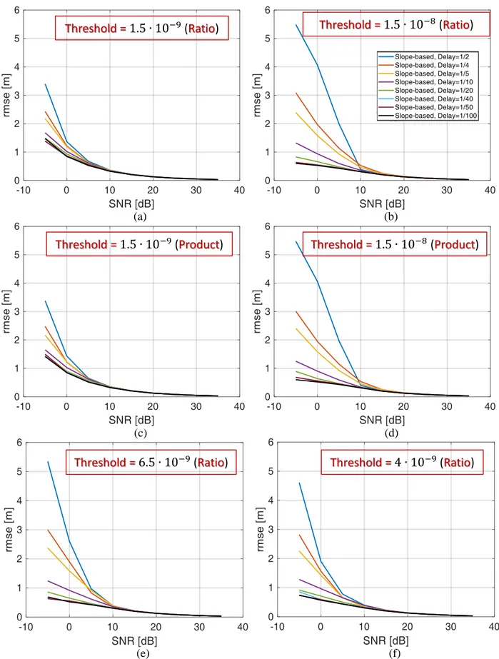
At this point it is sufficient to analyze the performance of the slope-based method for delays less than a sample, leaving to the CCF method to compensate for delays that are multiple of a sample. The analyses were conducted on a limited number of samples of the starting signals; in this case 1500 samples were used.
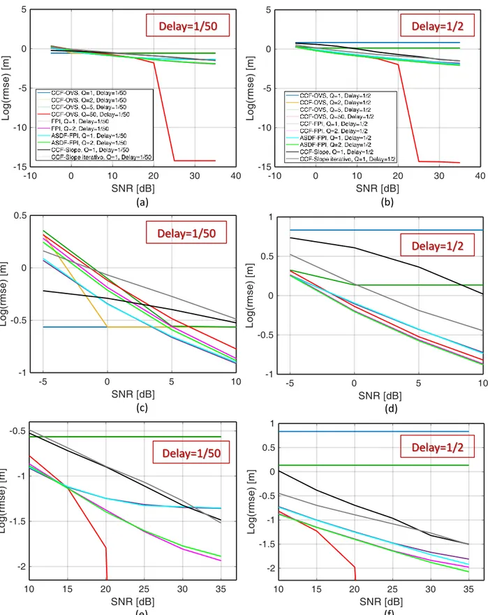
In Figure 2.10, we reported the Root Mean Square Error (RMSE) as a function of the signal-to-noise ratio (SNR). This figure shows that the trend of the obtained curves seems to be dependent on the relative delay between the two signals.
33
This behavior is not acceptable for our purposes and it is also interesting and necessary to understand the reason for this phenomenon. To do this, the phase of the ratio of the spectra of the starting signals has been analyzed in detail, each time obtained for a different SNR and for a different delay. As a consequence, being for us useful only the information related to the average slope of the phase, the latter has been approximated with a straight line (linear fitting) defined by the relative slope (angular coefficient), and its evolution has been observed as the noise increases.
To simplify the analysis, the phases (in blue) and the straight lines defined by the relative slopes (in red) are reported here (Figure 2.11) for only two cases which could be interesting for our study, i.e. the extreme cases of relative delay equal to half a sample and one fiftieth of a sample.
Figure 2.10. Rmse vs SNR of the slope-based method for different values of delay to be estimated.
34
Delay = 1/50, No Additive Noise Delay = 1/2, No Additive Noise
Delay = 1/50, SNR = 35 dB Delay = 1/2, SNR = 35 dB
Delay = 1/50, SNR = 10 dB Delay = 1/2, SNR = 10 dB
Delay = 1/50, SNR = -5 dB Delay = 1/2, SNR = -5 dB