Technical Report CoSBi 04/2006
Membrane Systems with Peripheral
Proteins: Transport and Evolution
Matteo Cavaliere
The Microsoft Research – University of Trento Centre for Computational and Systems Biology
Sean Sedwards
The Microsoft Research – University of Trento Centre for Computational and Systems Biology
This is a preliminary version of a paper that will appear in
Proceedings of MeCBIC06, Electronic Notes in Theoretical Computer Science, 171:2, 37–53, 2007.
Abstract
Transport of substances and communication between compartments are fun-damental biological processes, often mediated by the presence of opportune and complementary proteins attached to the surfaces of membranes. Within compart-ments, substances are acted upon by local biochemical rules.
Inspired by this behaviour we present a model based on membrane systems, with objects attached to the sides of the membranes and floating objects that can move between the regions of the system. Moreover, in each region there are evolution rules that rewrite the transported objects, mimicking chemical reactions. We first analyse the system, showing that interesting qualitative properties can be decided (like reachability of configurations) and then present a simulator based on a stochastic version of the introduced model and show how it can be used to simulate relevant quantitative biological processes.
1
Introduction and Motivations
Membrane systems are models of computation inspired by the structure and the function of biological cells. The model was introduced in 1998 by Gh. P˘aun and since then many results have been obtained, mostly concerning the computational power of the model (for an updated bibliography the reader can consult the web-page [23]). More recently, membrane systems have been applied to systems biology and several models have been proposed for simulating biological processes (e.g., see the monograph dedicated to membrane systems applications, [8]).
In the original definition, membrane systems are composed of an hierarchical nesting of membranes that enclose regions in which floating objects exist. Each region can have associated rules for evolving these objects (called evolution rules, modelling the biochem-ical reactions present in cell regions), and/or rules for moving objects across membranes (called symport/antiport rules, modelling some kind of transport rules present in cells). Recently, inspired by brane calculus, [4], a model of a membrane system, having objects attached to the membranes, has been introduced in [5]. Other models bridging brane cal-culus and membrane systems have been proposed in [14, 17]. A more general approach, considering both free floating objects and objects attached to the membranes has been proposed and investigated in [3]. The idea of these models is that membrane operations are moderated by the objects (proteins) attached to the membranes. However, in these models objects were associated to an atomic membrane which has no concept of inner or outer surface. In reality, many biological processes are driven and controlled by the presence, on the opportune side of a membrane, of certain specific proteins. For instance, receptor-mediated endocytosis, exocytosis and budding in eukaryotic cells are processes where the presence of proteins on the internal and external surface of a membrane is crucial (see e.g., [1]).
These processes are, for instance, used by eukaryotic cells to take up macromolecules and deliver them to digestive enzymes stored in lysosomes inside the cells. In general, all the compartments of a cell are in constant communication, with molecules being passed
from a donor compartment to a target compartment by means of numerous membrane-enclosed transport packages, or transport vesicles. Once transported to the correct com-partment the substances are then processed by means of local biochemical reactions (see e.g., [1]).
Motivated by this, we introduce a model combining some basic features found in biological cells: (i) evolution of objects (molecules) by means of multiset rewriting rules associated with specific regions of the systems (the rules model biochemical reactions); (ii) transport of objects across the regions of the system by means of rules associated with the membranes of the system and involving proteins attached to the membranes (in one or possibly both the two sides) and (iii) rules that take care of the attachment/de-attachment of objects to/from the sides of the membranes. Moreover, since we want to distinguish the functioning of different regions, we also associate to each membrane a unique identifier (a label).
In this paper we present a preliminary qualitative investigation of the model when the evolution is based on a sort of free parallelism: we prove that in this case several interesting problems, like configuration reachability, can be decided. We also introduce a stochastic variant of the model (i.e., where each rule has an associated rate) that underlies an implemented simulator which we have used to model interesting biological cellular processes.
We wish to comment that the model presented follows the philosophy of the evolution-communication model introduced in [6], where the system evolves by evolution of the objects and transport of objects by means of symport/antiport rules, that are essentially synchronized exchanges of objects. However, in our case the transport of objects may depend on the presence of particular proteins attached to the internal and external sur-faces of the membranes. Therefore this paper can be seen as a bridge between membrane systems and projective brane calculus, [9], where, in the framework of process algebra, directed actions associated to membranes have been considered.
2
Formal Language Preliminaries
We will briefly recall the main notions and results of the formal language theory used in this paper. For more details the reader can consult standard books, such as [12], [22], [10], and the respective chapters of the handbook [21].
Given a set A, we denote by |A| its cardinality. The empty set is denoted by ∅.
As usual, an alphabet V is a finite set of symbols. By V∗ we denote the set of all strings over V . The empty string is denoted by λ.
The length of a string w ∈ V∗ is denoted by |w|, while the number of occurrences of a ∈ V in w is denoted by |w|a. The notation P erm(x) indicates the set of all strings
that can be obtained as a permutation of the string x.
For x, y ∈ V∗ we define their shuffle by xξy = {x1y1· · · xnyn | x = x1· · · xn, y =
y1· · · yn, xi, yi ∈ V∗, 1 ≤ i ≤ n, n ≥ 1}. The operation can be extended in a natural way
Denoting by REG the family of regular languages, the following result holds (see e.g., [21]) (proved in a constructive way).
Theorem 2.1 L1, L2 ∈ REG, then L1ξL2 ∈ REG
A multiset over a set V is a map M : V → N, where M (a) denotes the multiplicity of the symbol a ∈ V in the multiset M . This fact can also be indicated in the forms (a, M (a)) or aM (a), for all a ∈ V . If the set V is finite, e.g. V = {a
1, . . . , an}, then the multiset M
can be explicitly described as {(a1, M (a1)), (a2, M (a2)), . . . , (an, M (an))}. The support
of a multiset M is the set supp(M ) = {a ∈ V | M (a) > 0}. A multiset is empty (so finite) when its support is empty (also finite).
A compact notation can be used for finite multisets: if M = {(a1, M (a1)), (a2, M (a2)),
. . . , (an, M (an))} is a multiset of finite support, then the string w = a M (a1) 1 a M (a2) 2 . . . a M (an) n
(and all its possible permutations) precisely identify the symbols in M and their multi-plicities. Hence, given a string w ∈ V∗, we can assume that it identifies a finite multiset over V defined by M (w) = {(a, |w|a) | a ∈ V }.
In this paper we make use of the notion of a matrix grammar.
A matrix grammar with appearance checking (ac) is a construct G = (N, T, S, M, F ), where N, T are disjoint alphabets of non-terminal and terminal symbols, S ∈ N is the axiom, M is a finite set of matrices, which are sequences of context-free rules of the form (A1 → x1, . . . , An → xn), n ≥ 1, (with Ai ∈ N, xi ∈ (N ∪ T )∗, in all cases), and F is a
set of occurrences of rules in M .
For w, z ∈ (N ∪ T )∗ we write w =⇒ z if there is a matrix (A1 → x1, . . . , An → xn)
in M and strings wi ∈ (N ∪ T )∗, 1 ≤ i ≤ n + 1, such that w = w1, z = wn+1, and, for all
1 ≤ i ≤ n, either
(i) wi = w0iAiw00i, wi+1= wi0xiwi00, for some wi0, w00i ∈ (N ∪ T )∗
or
(ii) wi = wi+1, Ai does not appear in wi, and the rule Ai → xi appears in F .
The rules of a matrix are applied in order, possibly skipping the rules in F if they cannot be applied (one says that these rules are applied in appearance checking mode).
The family of languages generated by matrix grammars with appearance checking is denoted by M ATac.
G is called a matrix grammar without appearance checking if and only if F = ∅. In this case, the generated family of languages is denoted by M AT .
If we denote by CF , and RE the family of context-free and recursively enumerable languages, respectively, then the following results hold:
Theorem 2.2
• CF ⊂ M AT ⊂ RE • M AT ⊂ M ATac = RE
A matrix grammar is called pure if there is no distinction between terminals and non-terminals. The language generated by a pure matrix grammar is composed of all the sentential forms. The family of languages generated by pure matrix grammars without appearance checking is denoted by pM AT . A proof of this can be found, for example, in [10].
Theorem 2.3 pM AT ⊂ M AT
In what follows we assume the reader to be familiar with the basic notions of membrane systems, for instance, as presented in the introductory guide [20].
3
Membrane Operations with Peripheral Proteins
As is usual in the membrane systems field, a membrane is represented by a pair of square brackets, [ ]. To each topological side of a membrane we associate multisets u and v (over a particular alphabet V ) and this is denoted by [ u]v. We say that the membrane
is marked by u and v; v is called the external marking and u the internal marking; in general, we refer to them as markings of the membrane. The objects of the alphabet V are called proteins or, simply, objects. An objects is called free if it is not attached to the sides of a membrane, so is not part of a marking.
Each membrane encloses a region and the contents of a region can consist of free objects and/or other membranes (we also say that the region contains free objects and/or other membranes).
Moreover, each membrane has an associated label that is written as a superscript of the membrane. If a membrane is named by the label i we can call it membrane i. Each membrane encloses a unique region, so we also say region i to identify the region enclosed by membrane i. The set of all labels is denoted by Lab.
For instance, in the system [ abb [ aaaa ab]1b bba]2ab, the external membrane, labelled by
2, is marked by bba (internal marking) and by ab (external marking). The contents of the region enclosed by the external membrane is composed of the free objects a, b, b and the membrane [ aaaaab]1b.
We consider rules that model the attachment of objects to the sides of the membranes. These rules extend the definition given in [3].
attach : [ au]iv → [ua]iv, a[u]iv → [u]iva
de − attach : [ ua]iv → [au]iv, [u]iva → [u]iva
with a ∈ V , u, v ∈ V∗ and i ∈ Lab.
The semantics of the attachment rules is as follows. For the first case, the rule is applicable to the membrane i if the membrane is marked by multisets containing the multisets u and v, on the appropriate sides, and region i contains the object a. In the second case, the rule is applicable to membrane i if it is marked by multisets containing the multisets u and v, as before, and is contained in a region that contains the object a.
When either rule is executed, the object a is added to the appropriate marking in the way specified. The objects not involved in the application of a rule are left unchanged in their original positions.
The semantics of the de-attachment rules is similar, with the difference that the attached object a is detached from the specified marking and added to the contents of either the internal or external region.
We now consider rules associated to the membranes that control the passage of objects across the membranes.
movein : a[ u]iv → [ au]iv
moveout : [ au]iv → a[ u]iv
with a ∈ V , u, v ∈ V∗ and i ∈ Lab.
The semantics of the rules is as follows. In the first case, the rule is applicable to membrane i if it is marked by multisets containing the multisets u and v, on the appropriate sides, and the membrane is contained in a region containing the object a. When the rule is executed the object a is removed from the contents of the region surrounding membrane i and added to the contents of region i.
In the second case the semantics is similar, but here the object a is moved from region i to its surrounding region.
The rules of attach, de-attach, movein, moveout are generally called membrane rules
over the alphabet V and the set of labels Lab.
We also introduce evolution rules that involve objects but not membranes. These can be considered to model the biochemical reactions that take place inside the compartments of the cell. They are evolution rules over the alphabet V and set of labels Lab and they follow the definition that can be found in evolution-communication P systems [6].
evol : [u → v]i
with u ∈ V+, v ∈ V∗ and i ∈ Lab. The evolution rule is called cooperative (coo) if |u| > 1,
otherwise the rule is called non-cooperative (ncoo).
The semantics of the rule is as follows. The rule is applied to region i if the region contains a multiset of free objects that includes the multiset u. When the rule is executed the objects specified by u are subtracted from the contents of region i and the objects specified by v are added to the contents of the region i.
4
Membrane Systems with Peripheral Proteins
In this section we define membrane systems having membranes marked with multisets of proteins on both sides of the membrane, free objects and using the operations introduced in Section 3.
Formally, a membrane system with peripheral proteins (in short, a Ppp system) and n
membranes, is a construct
Π = (V, µ, (u1, v1) . . . , (un, vn), w1, . . . , wn, R, Rm)
• V is a finite, non-empty alphabet of objects (proteins).
• µ is a membrane structure with n ≥ 1 membranes, injectively labelled by 1, 2, · · · , n. • (u1, v1), · · · , (un, vn) ∈ V∗ × V∗ are the markings associated, at the beginning of
any evolution, to the membranes 1, 2, · · · , n, respectively. They are called initial markings of Π; the first element of each pair specifies the internal marking, while the second one specifies the external marking.
• w1, · · · , wn specify the multisets of free objects contained in regions 1, 2, · · · , n,
respectively, at the beginning of any evolution and they are called initial contents of the regions.
• R is a finite set of evolution rules over V and the set of labels Lab = {1, . . . , n}. • Rm is finite set of membrane rules over the alphabet V and set of labels Lab =
{1, . . . , n}.
A configuration of Π consists of a membrane structure, the markings (internal and external) of the membranes and the multisets of free objects present inside the regions. In what follows, configurations are denoted by writing the markings as subscripts (in-ternal and ex(in-ternal) of the parentheses which identify the membranes, the labels of the membranes are written as superscripts and the contents of the regions as string, e.g.,
[ [ aa]1ab [aaaaa]2b [ b ]3bb a ]4a
We suppose a standard labelling: 0 is the label of the environment that surrounds the entire system Π; 1 is the label of the skin membrane that separates Π from the environment.
The initial configuration consists of the membrane structure µ, the initial markings of the membranes and the initial contents of the regions; the environment is empty at the beginning of the evolution.
We assume the existence of a clock which marks the timing of steps (single transitions) for the whole system.
A single transition of Π from a configuration to a new one is performed by applying an arbitrary number of membrane and evolution rules. This implies that, in one step, no rule, one rule, or as many as rules as desired may be applied in a non-deterministic way (i.e., so-called free parallelism) and all rules have equal precedence.
A sequence of transitions, starting from the initial configuration, is called an evolution. An evolution is said to be halting if it halts, that is, if it reaches a halting configuration, i.e., a configuration where no rule can be applied anywhere in the system.
A configuration of a Ppp system Π that can be reached by a sequence of transitions,
reachable marking for Π if there exists a reachable configuration of Π which contains at least one membrane marked internally by u and externally by v. We denote by C(Π) the set of all possible configurations of Π, by CR(Π) the set of all reachable configurations of
Π, and by MR(Π) the set of all reachable markings of Π.
Moreover we denote by Ppp,m(memrul, α), α ∈ {coo, ncoo} the class of membrane
systems with peripheral proteins, membrane rules, evolution rules of type α and m mem-branes (m is changed to ∗ if it is unbounded). We omit memrul or α from the notation if
the corresponding type of rules is not allowed. We also denote by VΠ the alphabet V of
the system Π. The notion of free parallelism we use here is similar to the one introduced in ([19], Chapter 3.4).
5
Reachability of Configurations and Markings
A natural question with possible biological implications concerns whether or not a system can evolve to a particular specified configuration. Hence it would be useful to construct models having such qualitative properties, to be decidable.
In our case, we can prove that it is possible to decide, for an arbitrary membrane system with peripheral proteins and an arbitrary configuration, whether or not such a configuration is reachable. A proof can be demonstrated by showing that all the reachable configurations of a system Π can be produced by a pure matrix grammar without ap-pearance checking. Moreover, we also prove that the reachability of an arbitrary marking can be decided.
Lemma 5.1 It is decidable whether or not, for any P system Π from Ppp,1(coo) and any configuration C of Π, C ∈ CR(Π)
Proof Let Π = (V, µ = [ ]1, (u1, v1), w1, R). We first notice that each configuration C
of Π is essentially the contents of the unique region and therefore, being a multiset, it can be represented by a string wC, as described in Section 2 (every permutation of the
string wC represents the same contents, so the same configuration C). We construct a
pure matrix grammar G without appearance checking such that L(G) contains all and only the strings representing the configurations in CR(Π).
The grammar G = (N, S, M ) is defined in the following way. N = V ∪ V#, with V# = {v# | v ∈ V }. We add to M the following matrices. (S → w
1) and, for each rule
[x → y]1 ∈ R, the matrix (x1 → x # 1, x2 → x # 2, · · · , xk → x # k, x # 1 → λ, x # 2 → λ, · · · , x # k → y1y2· · · yq)
where x = x1x2· · · xk and y = y1y2· · · yq. Each application of a matrix simulates the
application of an evolution rule inside the unique region of the system. The markings are not involved in the evolution of the system since membrane rules are not allowed. It is immediate that, for each string w in L(G) (i.e., all the sentential forms generated by G) there is an evolution of Π, starting from the initial configuration, that reaches the configuration represented by w. Moreover it is easy to see that it is true also the reverse since the evolution of Π is based on free parallelism: for each reachable configuration
C0 of Π there exists a derivation of G that generates a string representing C0. In fact it is immediate to see that L(G) contains all the strings representing configurations of Π reached by applying at each step a single evolution rule. In case a configuration C0 is reached by applying more than an unique evolution rule in a single step, then such single step can be simulated in G by applying an opportune sequence of matrices (because the evolution of Π is based on free parallelism).
Therefore to check whether or not an arbitrary configuration C of Π can be reached, we only need to check if any of the strings representing C is in L(G). This can be done since there is only a finite number of strings representing C and the membership problem for pure matrix grammars without appearance checking is decidable (see, e.g.,
[10]); therefore the Lemma follows. 2
Theorem 5.1 It is decidable whether or not, for any P system Π from Ppp,∗(memrul, coo)
and any configuration C of Π, C ∈ CR(Π)
Sketch Proof The main idea of the proof is that the problem can be reduced to check whether or not a configuration of a system from Ppp,1(coo) is reachable, and this is
decidable (Lemma 5.1).
Suppose Π = (V, µ, (u1, v1) . . . , (un, vn), w1, . . . , wn, R, Rm). By cont(i) we denote the
la-bel of the region surrounding membrane i (we recall that 0 is the lala-bel of the environment and 1 is the label of the skin membrane).
We construct Π = (V , [ ]1, (λ, λ), w1, R) from Ppp,1(coo) in the following way.
We define V =S i∈{1,··· ,n}(V 0 i ∪ V 00 i ) ∪ S i∈{0,1,··· ,n}Vi with Vi = {ai | a ∈ V }, V 0 i = {a 0 i | a ∈ V }, Vi00 = {a00i | a ∈ V }.
We use the morphisms hi, h0i, h 00
i, defined as follows.
• hi : V → Vi defined by hi(a) = ai, a ∈ V , for i ∈ {0, 1, · · · , n}
• h0 i : V → V 0 i defined by h 0 i(a) = a 0 i, a ∈ V , for i ∈ {1, · · · , n} • h00 i : V → V 00 i defined by h 00 i(a) = a 00 i, a ∈ V , for i ∈ {1, · · · , n}
We define w1 as the string h1(w1) · · · hn(wn)h01(u1) · · · h0n(un)h001(v1) · · · h00n(vn).
For each rule movein, a[ u]iv → [ a u]iv ∈ Rm, i ∈ {1, · · · , n} we add to R the following
rules: [ akh0i(u)h 00
i(v) → aih0i(u)h 00
i(v)]1, with k = cont(i).
In the same way all the other rules present in R∪Rmcan be translated in the evolution rules for R.
Hence, given a configuration C of Π, one can construct the configuration C of Π having a unique region in the following way.
For each occurrence of free object a contained in region i (the environment if i = 0) in C, i ∈ {0, 1, · · · , n} we add the object hi(a) in region 1 of C. For each occurrence of
object a present in the internal marking of membrane i in C, i ∈ {1, · · · , n} we add the object h0i(a) to region 1 of C and finally for each occurrence of object a present in the
external marking of membrane i, i ∈ {1, · · · , n} we add the object h00i(a) to region 1 of C .
Now we can decide (Lemma 5.1) whether or not C ∈ CR(Π).
From the way Π has been constructed it follows that: • if C ∈ CR(Π) then C ∈ CR(Π)
• if C /∈ CR(Π) then C /∈ CR(Π)
and from this the Theorem follows.
Corollary 5.1.a It is decidable whether or not, for any P system Π from Ppp,n(memrul, coo), n ≥
1 and any pair of multisets (u, v) over VΠ, (u, v) ∈ MR(Π).
Proof Given Π from Ppp,n(memrul, coo) and with alphabet of objects V , one can
con-struct Π = (V , µ = [ ]1, (λ, λ), w1, R) from Ppp,1(coo) in the way described by Theorem
5.1.
Therefore, using Π one can construct the grammar G as described by Lemma 5.1 such that L(G) contains all and only the strings representing the configurations in CR(Π).
Now to check whether or not an arbitrary (u, v) ∈ MR(Π) one needs to check whether
or not there exists an i ∈ {1, · · · , n} such that
(P erm(h0i(u))ξ(V )∗) ∩ L(G) 6= ∅ and (P erm(h00i(v))ξ(V )∗) ∩ L(G) 6= ∅, where h0i and h00i are morphisms from V to Vi0 and to Vi00, respectively, defined as in Theorem 5.1, and ξ denotes the shuffle operation.
The permutation and shuffle operation are used to construct all possible strings rep-resenting a configuration of Π containing the membrane i is marked by u internally and v externally.
The languages (P erm(h0i(u))ξ(V )∗) ∩ L(G) and (P erm(h00i(v))ξ(V )∗) ∩ L(G) can be generated by matrix grammars without appearance checking (see, Theorem 2.1 and e.g., [10]) and the emptiness problem for this class of grammars is decidable (see, e.g., [10]).
Therefore the Corollary follows. 2
6
Stochastic Simulation of Yeast G-protein Cycle
Having defined a qualitative model, we wish to use it to examine quantitative properties of biological systems using a simulator.
Deterministic simulations are useful to describe reactions between large numbers of chemical objects, however they may not accurately represent the dynamical behaviour of small quantities of reactants. In this latter case a discrete stochastic simulation is more appropriate and, moreover, approximates the deterministic approach when the quantities are increased [11]. Hence we have created a simulator [24] based on the presented model, which assumes discrete molecular interactions and uses the Gillespie algorithm [11] to stochastically choose at each step which single rule to apply (in one of the regions) and to
calculate its stochastic time delay. Thus the more general free parallel theoretical model is here reduced to a specific sequential one.
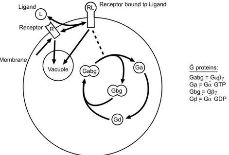
To demonstrate the simulator we model the G-protein mating response in yeast sac-charomyces cerevisiae, based on experimental rates provided by [13]. The G-protein transduction pathway involves membrane proteins and the transport of substances be-tween regions and is a mechanism by which organisms detect and respond to environ-mental signals. It is extensively studied and many pharmaceutical agents are aimed at components of the G-protein cycle in humans. Figure 1 shows the relationships between the various reactants and regions modelled in the simulation, Figure 2 is the simulation script and Figure 3 shows the results of the simulation.
Vacuole L
Ligand
R Receptor
RL Receptor bound to Ligand
Membrane Débora Gabg Gbg Ga Gd G-proteins: Gabg = Gabg Ga = Ga-GTP Gbg = Gbg Gd = Ga-GDP
Figure 1: Model of saccharomyces cerevisiae mating response.
A brief description of the process is that the yeast cell receives a pheromone signal (L) which binds to receptor R, integral to the cell membrane. The receptor-ligand dimer then catalyses the reaction that converts the inactive G-protein Gabg to the active Ga. A competing sequence of reactions converts Ga to Gabg via Gd in combination with Gbg. The bound and unbound receptor (RL and R, respectively) are degraded by transport into a vacuole via the cytoplasm.
7
Prospects
We have introduced a model of membrane systems with objects attached to both sides of the membranes. In addition, the model is equipped with operations that can rewrite floating objects and move objects between regions depending on the attached objects. We have proved that when the system works in a free parallelism mode (i.e., allowing an arbitrary number of rules to be applied at each step) many useful properties can be decided (for instance, reachability of a configuration or of a certain protein marking).
// Saccharomyces cerevisiae G-protein mating response molecule L,R,RL,Gd,Gbg,Gabg,Ga rule g cycle { || 4-> |R| |R| + L 3.32e-18-> |RL| |RL| 0.011-> |R| + L |RL| 4.1e-3-> RL + || |R| 4.1e-4-> R + ||
Gabg + |RL| 1.0e-5-> Ga, Gbg + |RL| Gd + Gbg 1-> Gabg
Ga 0.11-> Gd }
rule vac rule {
|| + R 4.1e-4-> R + || || + RL 4.1e-3-> RL + || }
compartment vacuole [vac rule]
compartment cell [vacuole, 3000 Gd, 3000 Gbg, 7000 Gabg, g cycle : ... |10000 R|] system cell, 6.022e17 L
evolve 0-600000
plot cell[Gd,Gbg,Gabg,Ga:|R,RL|]
Figure 2: Simulation script of G-protein cycle using data from [13].
In the second part of the paper we have presented a simulator that implements a stochastic variant of the introduced model. The simulator has an intuitive syntax and can be used to model biological processes where the transport of objects across membranes is coupled with the processing/decay of substances within the regions. As an example we have presented the simulation of saccharomyces cerevisiae heterotrimeric G-protein cycle.
Several different research directions may now be pursued. The model may be further developed, for example, to include evolution based on maximal parallel semantics, as commonly used in P systems. In that case it is most likely that many properties would not be decidable; an interesting problem is then to find (sub)classes (using restricted evolution and/or transport rules, say) where interesting properties are still decidable. Additionally, other bio-inspired operations may be introduced, such as fission and fusion of regions, all still dependent on the objects attached to the membranes, along the lines of the research found in [17].
Another direction of research is the application of the existing model. The imple-mented stochastic software can be used to simulate interesting biological processes where the rˆole of surface proteins and transport of substances is crucial (as in drug-resistance, see e.g.,[16]).
10000 molecules 8000 6000 4000 2000 0 0 100 200 300 400 500 600 seconds Gabg Gbg, Ga R RL
Figure 3: Simulation results (continuous curves) and experimental data (points with error bars, [13]) corresponding to simulated Ga. Note that Gd decays rapidly and is not visible at this scale.
References
[1] B. Alberts, Essential Cell Biology. An Introduction to the Molecular Biology of the Cell. Garland Publ. Inc., New York, London, 1998.
[2] N. Busi, R. Gorrieri, On the Computational Power of Brane Calculi. Proceedings Third Workshop on Computational Methods in Systems Biology. Edinburgh, 2005.
[3] R. Brijder, M. Cavaliere, A. Riscos-N´u˜nez, G. Rozenberg, D. Sburlan, Membrane Systems with
Marked Membranes. Submitted.
[4] L. Cardelli, Brane Calculi. Interactions of Biological Membranes. Proceedings Computational
Meth-ods in System Biology 2004 (V. Danos, V. Sch¨achter, eds.), Lecture Notes in Computer Science,
3082, Springer-Verlag, Berlin, 2005, pp. 257–278.
[5] L. Cardelli, Gh. P˘aun, An Universality Result for a (Mem)Brane Calculus Based on Mate/Drip
Operations. Proceedings of the ESF Exploratory Workshop on Cellular Computing (Complexity
Aspects), (M.A. Guti´errez-Naranjo, Gh. P˘aun, M.J. P´erez-Jim´enez, eds.), F´enix Ed., Seville, Spain,
pp. 75–94. Also at http://www.gcn.us.es/.
[6] M. Cavaliere, Evolution-Communication P Systems. Proceedings International Workshop Membrane
Computing, (Gh. P˘aun, G. Rozenberg, A. Salomaa, C. Zandron eds.), Lecture Notes in Computer
Science, 2597, Springer-Verlag, Berlin, 2003, pp. 134–145.
[7] M. Cavaliere, D. Sburlan, Time-Independent P Systems. Membrane Computing, 5th International
Workshop, WMC2004 (G. Mauri, Gh. P˘aun, M.J. P´erez-Jim´enez, G. Rozenberg, A. Salomaa, eds.),
Lecture Notes in Computer Science, 3365, Springer-Verlag, Berlin, 2005, pp. 239–258.
[8] G. Ciobanu, Gh. P˘aun, M.J. P´erez-Jim´enez, eds., Applications of Membrane Computing.
[9] V. Danos, S. Pradalier, Projective Brane Calculus. Proceedings Computational Methods in System
Biology 2004 (V. Danos, V. Sch¨achter, eds.), Lecture Notes in Computer Science, 3082,
Springer-Verlag, Berlin, 2005, pp. 134–148.
[10] J. Dassow, Gh. P˘aun, Regulated Rewriting in Formal Language Theory. Springer-Verlag, Berlin,
1989.
[11] D. T. Gillespie, Exact Stochastic Simulation of Coupled Chemical Reactions, Journal of Physical Chemistry, 81, 25, 1977.
[12] J.E. Hopcroft, J.D. Ullman, Introduction to Automata Theory, Languages, and Computation. Addison-Wesley, 1979.
[13] T.-M. Yi, H. Kitano, M. I. Simon, A quantitative characterization of the yeast heterotrimeric G protein cycle, Proceedings of the National Academy of Science, 100, 19, 2003.
[14] S.N. Krishna, Universality Results for P Systems based on Brane Calculi Operations. Theoretical Computer Science, to appear.
[15] H. Lodish, A. Berk, S.L. Zipursky, P. Matsudaira, D. Baltimore, J. Darnell, Molecular Cell Biology, Freeman, Fifth Edition.
[16] K. H. Lundstrom, G Protein Coupled Receptors in Drug Discovery, Taylor & Francis, 2005.
[17] A. P˘aun, B. Popa, P Systems with Proteins on Membranes and Membrane Division. Proceedings
Tenth International Conference in Developments in Language Theory, DLT06, Lecture Notes in Computer Science, Springer-Verlag, to appear.
[18] Gh. P˘aun, Computing with Membranes. Journal of Computer and System Sciences, 61, 1 (2000),
pp. 108–143. First circulated as TUCS Research Report No 28, 1998.
[19] Gh. P˘aun, Membrane Computing – An Introduction. Springer-Verlag, Berlin, 2002.
[20] Gh. P˘aun, G. Rozenberg, A Guide to Membrane Computing. Theoretical Computer Science, 287-1
(2002), pp. 73–100.
[21] G. Rozenberg, A. Salomaa, eds., Handbook of Formal Languages. Springer-Verlag, Berlin, 1997. [22] A. Salomaa, Formal Languages. Academic Press, New York, 1973.
[23] http://ppage.psystems.eu
[24] http://www.cosbi.eu/rpty_soft_cytosim.php Revised 30/9/09
A
Appendix - The Simulator Syntax
An example of the basic syntax of the simulator is shown in the following script:
// Lotka autocatalytic reactions [Journal Am Ch Soc, 1920] molecule X,Y1,Y2,Z
rule r1 X + Y1 0.0002-> 2Y1 + X rule r2 Y1 + Y2 0.01-> 2Y2 rule r3 Y2 10-> Z
system 100000 X, 1000 Y1, 1000 Y2, r1,r2,r3 evolve 0-50000000
plot Y1,Y2
The reacting species are first listed in the type definition beginning with the keyword
molecule.
The behaviour of the reactants is then defined using rule definitions comprising the keyword rule followed by a rule identifier and the rewriting rule itself. Note that rules are user-defined types which may be instantiated more than once. The value preceding the implication symbol (->) is the average reaction rate.
It is also possible to define a rule as a group of rules. E.g.,
rule lotka {
r1 X + Y1 0.0002-> 2Y1 + X rule r2 Y1 + Y2 0.01-> 2Y2 rule r3 Y2 10-> Z
}
uses the single identifierlotka to define the behaviour described by r1, r2and r3 in the
previous example. Such groups are convenient to describe a subsystem of behaviour. The system is instantiated using thesystemkeyword followed by a list of constituents, in the above case comprising numbers of molecules and rules.
The number of reactions to simulate is specified using the evolve keyword followed by the range of data points to record. The simulation will always proceed from zero to the maximum value, however data will only be recorded from the minimum given.
The species to be observed are defined using the plot keyword followed by a list of reactants.
Enclosed regions, subsequently referred to as compartments, may be defined using the keywordcompartmentfollowed by an identifier and a list of contents and rules, all enclosed by square brackets. For example,
compartment c1 [100 X, 100 Y1, r1, r2]
instantiates a compartment having the labelc1containing 100X, 100Y1and rules r1and r2. Compartments may contain other compartments, so the following is possible given the previous definition:
Compartments contain a notional membrane which surrounds them and to which may be attached reactants. The compartment syntax is thus extended using the symbol ||
to represent the membrane. Hence,
compartment c3 [100 X, c2 : 10 Y2||10 Y1]
has the meaning that the compartment c3 contains 100 X, compartment c2 and the membrane surrounding c3 has 10 Y2 attached to its inner surface and 10 Y1 attached to its outer surface. Note that the list of floating contents and rules appears on the left of the definition and is separated from the membrane contents by a :. The rule syntax is correspondingly extended, so
rule r4 X + Y2|| 0.1-> Y2|| + X
means that if one X exists within the compartment and one Y2 exists attached to the inner surface of the membrane, then the X will be transported outside the compartment
and the state of the membrane will be unaffected. Hence the + is non-commutative:
the left side represents the internal part of the compartment and the right hand side is external. Similarly, the left side of the || symbol represents the internal surface and the
right hand side represents the external surface of the membrane. Reactants integral to the membrane (not specifically mentioned in the previous text) may be defined by listing them between the vertical bars, so
rule r5 X + |Y2| 0.1-> |Y2| + X
represents exocytosis where Y2 must exist integral to the membrane for the reaction to proceed.
To plot the contents of a specific compartment theplotstatement uses syntax similar
to that used in the compartment definition. E.g.,
plot X, c3[X,Y1 : Y1|Y2|]
records the number of free-floating X in the system environment and also the contents of compartment c3. Specifically, it records the number of free-floating Xand Y1 inc3 as well as the number of Y1 attached to the inner surface and the number of Y2 integral to
the membrane.
The simulator is available for free download at
![Figure 2: Simulation script of G-protein cycle using data from [13].](https://thumb-eu.123doks.com/thumbv2/123dokorg/2954746.24633/12.892.125.669.171.615/figure-simulation-script-g-protein-cycle-using-data.webp)
![Figure 3: Simulation results (continuous curves) and experimental data (points with error bars, [13]) corresponding to simulated Ga](https://thumb-eu.123doks.com/thumbv2/123dokorg/2954746.24633/13.892.205.693.162.511/figure-simulation-results-continuous-curves-experimental-corresponding-simulated.webp)
