Investigation of petabyte-scale data transfer performances with PhEDEx for the CMS experiment

(1)

Alma Mater Studiorum · Università di Bologna

Scuola di Scienze Corso di Laurea in Fisica

Investigation of Petabyte-scale data

transfer performances with PhEDEx

for the CMS experiment

Relatore:

Prof. Daniele Bonacorsi

Presentata da:

Tommaso Diotalevi

Sessione II

(2)

(3)

Quo usque tandem abutere, Catilina, patientia nostra? [Cicerone, Oratio ad Catilinam I]

(4)

(5)

Sommario

PhEDEx, il sistema di gestione dei trasferimenti di CMS, durante il primo Run di LHC ha trasferito all’incirca 150 PB ed attualmente trasferisce circa 2.5 PB di dati alla settimana attraverso la Worldwide LHC Computing Grid (WLCG). Questo sistema è stato progettato per completare ogni trasferimento richiesto dall’utente a spese del tempo necessario per il suo completamento. Dopo svariati anni di operazioni con tale strumento, sono stati raccolti dati relativi alle latenze di trasferimento ed immagazzinati in log files contenenti informazioni utili per l’analisi. A questo punto, partendo dall’analisi di una ampia mole di trasferimenti in CMS, è stata effettuata una suddivisione di queste latenze ponendo particolare attenzione nei confronti dei fattori che contribuiscono al tempo di completamento del trasferimento.

L’analisi presentata in questa tesi permetterà di equipaggiare PhEDEx con un insieme di utili strumenti in modo tale da identificare proattivamente queste latenze e adottare le opportune tattiche per minimizzare l’impatto sugli utenti finali.

Il Capitolo 1 fornisce una panoramica di LHC, con maggiore attenzione all’esperimento

CMS.

Il Capitolo 2 descrive le basi del CMS Computing Model, il sistema di gestione

dei dati e le relative infrastrutture.

Il Capitolo 3 offre una visione d’insieme sul problema delle latenze di

trasferi-mento e ne descrive una suddivisione di diverse categorie.

Il Capitolo 4 analizza i dati prodotti dal sistema di monitoraggio di PhEDEx.

(8)

(9)

Abstract

PhEDEx, the CMS transfer management system, during the first LHC Run has moved about 150 PB and currently it is moving about 2.5 PB of data per week over the Worldwide LHC Computing Grid (WLGC). It was designed to complete each transfer required by users at the expense of the waiting time necessary for its completion. For this reason, after several years of operations, data regarding transfer latencies has been collected and stored into log files containing useful analyzable informations. Then, starting from the analysis of several typical CMS transfer workflows, a categorization of such latencies has been made with a focus on the different factors that contribute to the transfer completion time. The analysis presented in this thesis will provide the necessary information for equipping PhEDEx in the future with a set of new tools in order to proactively identify and fix any latency issues.

Chapter 1 provides a global view of CMS experiment at LHC.

Chapter 2 describes the basics of the CMS computing Model, with a focus on the

data management system and related infrastructures.

Chapter 3 offers an overview of the transfer latency issue in CMS computing

oper-ations and describes a categorization of such latencies in different categories.

Chapter 4 gives an analysis of latency data produced by the PhEDEx monitoring

system.

(10)

(11)

Chapter 1 High energy physics at LHC

1.1 A general view of the Large Hadron Collider

The Large Hadron Collider (LHC) [1,2] is part of the CERN accelerator complex (see Figure1.1) [3], in Geneva, and it is the most powerful particle accelerator ever built. The particle beam is injected and accelerated by each element of a chain of accelerators, with a progressive increase of energy until the beam injection into LHC, where particles are accelerated up to 13 TeV (by LHC design, its nominal center-of-mass energy).

The LHC basically consists of a circular 27 km circumference ring, divided into eight independent sectors, designed to accelerate protons and heavy ions. These particles travel on two separated beams on opposite directions and in extreme vacuum conditions (see Section 1.1.1). Beams are controlled by superconductive electromagnets (see Section 1.1.2) , keeping them in their trajectory and bringing them to regime.

Some of the main LHC parameters are shown in Table1.1.

Figure 1.1: The accelerators chain at CERN. 1

(12)

2 CHAPTER 1. HIGH ENERGY PHYSICS AT LHC Table 1.1: Main technical parameters of LHC.

Quantity value

Circumference (m) 26 659

Magnets working temperature (K) 1.9

Number of magnets 9593

Number of principal dipoles 1232

Number of principal quadrupoles 392

Number of radio-frequency cavities per beam 8

Nominal energy, protons (TeV) 7

Nominal energy, ions (TeV/nucleon) 2.76 Magnetic field maximum intensity (T) 8.33 Project luminosity (cm−2s−1) 10 × 1034 Number of proton packages per beam 2808 Number of proton per package (outgoing) 1.1 × 1011 Minimum distance between packages (m) ∼7

Number of rotations per second 11 245

Number of collisions per second (millions) 600

1.1.1 The vacuum system

The LHC vacuum system [4] is, with more than 104 kilometers of vacuum ducts, one of the most advanced in the world. Basically it has two functions: the first is to avoid collisions between beam particles and air molecules inside the ducts, recreating an extreme vacuum condition (10−13_atm_{), as empty as interstellar space;} the other reason is to cancel heat exchange between components who needs low temperatures in order to work properly and maximize the efficiency.

The vacuum system is made out of three independent parts: • an isolated vacuum system for cryomagnets;

• an isolated vacuum system for Helium distribution line; • a vacuum system for beams.

1.1.2 Electromagnets

Electromagnets [5] are designed to guide beams along their path, modifying single particles trajectories as well as align them in order to increase collision probability. There are more than fifty different kind of magnets in LHC, amounting to approx-imately 9600 magnets. Main dipoles, the bigger ones, generate a magnetic field with a maximum intensity of 8.3 T. Electromagnets require a current of 11 850 A in conditions of superconductivity in order to reset energy losses due to resistance. This happens thanks to a system of liquid helium distribution that keeps magnets at a temperature of about 1.9 K. At this incredibly low temperatures, below that required to operate in conditions of superconductivity, helium became also super-fluid: this means an high thermal conductivity used consequently as a refrigeration system for magnets.

(13)

1.2. LHC DETECTORS 3

1.1.3 Radiofrequency cavities

Radiofrequecy cavities [1] [2] [6] are metallic chambers in which electromagnetic field is applied. Their primary purpose is to separate protons in packages and to focus them at the collision point, in order to guarantee an high luminosity and thus a large number of collisions.

Particles, passing through the cavity, feel the overall force due to electromagnetic fields and push them forwards along the accelerator. In this scenario, the ideally timed proton, with exactly the right energy, will see zero accelerating voltage when LHC is at nominal energy while protons with slightly different energies will be accelerated or decelerated sorting particle beams into "bunches". LHC has eight cavities per beam: each of which furnishes 2 MV at 400 MHz. The cavities work at 4.5 K and are grouped into four cryo-modules.

At regime conditions, each proton beam is divided into 2808 bunches, each con-taining about 1011 _{protons. Away from the collision point, the bunches are a few} cm long and 1 mm wide, and are compressed up to 16 nm near the latter. At full luminosity, packages are separated in time by 25 ns, thus resulting in about 600 million collisions per second.

1.2 LHC detectors

Along the LHC circumference, the particles collide in four beam intersection points, in which the four main LHC experiments are built. Each experiment has its own detector, designed and built to gather the fragments of the large number of collisions and reconstruct all physical processes that generated them.

In particular, the four major experiments installed at LHC are: • A Large Ion Collider Experiment (ALICE)

• A Toroidal LHC ApparatuS (ATLAS) • Compact Muon Solenoid (CMS) • Large Hadron Collider beauty (LHCb)

In addition, there are secondary experiments, among which: • Large Hadron Collider forward (LHCf)

• TOTal Elastic and diffractive cross section Measurement (TOTEM)

In the following sections, the LHC detectors are briefly introduced, with a major focus on the CMS experiment.

1.2.1 ALICE

ALICE [7, 8] is a detector specialized in heavy ions collisions. It is designed to study the physics of strongly interacting matter at extreme energy densities, where

(14)

4 CHAPTER 1. HIGH ENERGY PHYSICS AT LHC a phase of matter called "quark-gluon plasma" forms. At these conditions, similar to those just after the Big Bang, quark confinement no longer applies: studying the quark-gluon plasma as it expands and cools allows to gain insight on the origin of the Universe. Some ALICE specifications are illustrated in Table1.2.

The collaboration counts more than 1000 scientists from over 100 physics institutes in 30 countries (updated to October 2014)

Table 1.2: ALICE detector specifications: Dimensions length: 26 m, height: 16 m, width: 16 m

Weight 10 000 tons

Design central barrel plus single arm forward muon spectometer Cost of materials 115 MCHF

Location St. Genis-Pouilly, France

1.2.2 ATLAS

ATLAS [9, 10], is one of the two general-purpose detectors at LHC. Although its similarities with the CMS experiment regarding scientific goals, they have subdetectors based on different technology choices, and the design of the magnets is also different. Some specs are illustrated below in Table 1.3.

It is located in a cavern 100m underground near the main CERN site. About 3000 scientists from 174 institutes in 38 countries work on the ATLAS experiment (updated to February 2012).

Table 1.3: ATLAS detector specifications:

Dimensions length: 46 m, height: 25 m, width: 25 m

Weight 7000 tons

Design barrel plus andcaps Cost of materials 540 MCHF

Location Meyrin, Switzerland

1.2.3 CMS

CMS [11, 12], as well as ATLAS, is a general-purpose detector at LHC. Is built around a huge solenoid magnet with a cylindrical form able to reach a 4 T magnetic field. Its main characteristics are illustrated in Table1.4. In the next chapter, CMS will be discussed more specifically.

(15)

1.2. LHC DETECTORS 5

Table 1.4: CMS detector specifications:

weight 12 500 tons

Design barrel plus end caps Cost of materials 500 MCHF

Location Cessy, France

1.2.4 LHCb

The LHCb [13,14] experiment is specialized in investigating the slight differences between matter and antimatter by studying the quark bottom. Instead of ATLAS or CMS, LHCb uses a series of subdetectors to detect mainly forward particles: the first one is mounted near the collision point while the others are placed serially over a length of 20 meters.

Some specifications are illustrated below in Table1.5. About 700 scientists from 66 different institutes and universities work on LHCb experiment (updated to October 2013).

Table 1.5: LHCb detector specifications:

Height 5600 tons

Design forward spectometer with planar detectors Cost of materials 75 MCHF

Location Ferney-Voltaire, France

1.2.5 Other LHC experiments

Aside from ALICE, ATLAS, CMS and LHCb, a few details on LHC smaller experiments, LHCf and TOTEM, are given in the following. LHCf [15, 16] is a small experiment which uses particles thrown forward by p-p collisions as a source to simulate high energy cosmic rays. LHCf is made up of two detectors which sit along the LHC beamline, at 140 m either side of ATLAS collision point. They only weights 40 kg and measures (30 x 80 x 10) cm.

LHCf experiment involves about 30 scientists from 9 institutes in 5 countries (updated to November 2012).

TOTEM [17,18] experiment is designed to explore protons cross-section as they emerge from collisions at small angles. Detectors are spread across half a kilometre around the CMS interaction point in special vacuum chambers called "roman pots" connected to beam ducts, in order to reveal particles produced during the collision. TOTEM has almost 3000 kg of equipment and 26 "roman pot" detectors. It involves about 100 scientists from 16 institutes in 8 countries (updated to August 2014)

(16)

6 CHAPTER 1. HIGH ENERGY PHYSICS AT LHC

(a) Section view. (b) View along the plane perpendicular to beam direction.

Figure 1.2: Compact Muon Solenoid

1.3 The CMS experiment

The CMS main purpose is to explore the p-p physics at the TeV scale, including precision measurements of the Standard Model, as well as search for new physics. Its cylindrical concept is built on several layers and each one of them is dedicated to the detection of a specific type of particle.

About 4300 people including physicists, engineers, technicians and students work actively on CMS experiment (updated to February 2014)

1.3.1 The CMS detector: concept and structure

As mentioned above, the CMS detector is made up of different layers, as illustrated in Figure1.2. Each of them is designed to trace and measure the physical properties and paths of different kinds of subatomic particles. Furthermore, this structure is surrounded by a huge solenoid based on superconductive technologies, operating at 4.4 K and generating a 4 T magnetic field.

The first and inner layer of the CMS detector is called Tracker [12, pp. 26-89]: made entirely of silicon, is able to reconstruct the paths of high-energy muons, electrons and hadrons as well as observe tracks coming from the decay of very short-lived particles with a resolution of 10 nm.

The second layer consists of two calorimeters, the Electromagnetic Calorimeter (ECAL) [12, pp. 90-121] and the Hadron Calorimeter (HCAL) [12, pp. 122-155] arranged serially. The former measures the energy deposited by photons and electrons, while the latter measures the energy deposited by hadrons.

Unlike the Tracker, which does not interfere with passing particles, the calorimeters are designed to decelerate and stop them.

In the end, a superconductive coil alternated with muon detectors [12, pp. 162-246] are able to track muon particles, escaped from calorimeters. The lack of energy and momentum from collisions is assigned to the electrically neutral and weakly-interacting neutrinos.

(17)

1.3. THE CMS EXPERIMENT 7 Tracker

The Tracker is a crucial component in the CMS design as it measures particles momentum through their path: the greater is their curvature radius across the magnetic field, the greater is their momentum. As stated above, the Tracker is able to reconstruct muons, electrons and hadrons path as well as tracks produced by short-lived particles decay, such as quark beauty. It has a low degree of interference with particles and a high resistance to radiations. Located in the inner part of the detector, it receives the greatest amount of particles. Interference with particles occur only in few areas of the Tracker with a resolution of about 10 nm.

This layer (Figure 1.3a) is entirely made of silicon: internally there are three levels of pixel detectors, after that particles pass through 10 layer of strip detectors, until a 130 cm radius from the beam pipe.

The pixel detector, Figure 1.3b, contains about 65 millions of pixels, with three levels of respectively 4, 7 e 11 cm radius. The flux of particles at this radius is maximum: at 8 cm is about 106 _{particles/cm·sec. Each level is divided into small} units, each one containing a silicon sensor of 150 nm × 150 nm. When a charged particle goes through one of this units, the amount of energy releases an electron with the consequent creation of an hole. This signal is than received by a chip which amplifies it. It is possible, in the end, to reconstruct a 3-D image using bi-dimensional layers for each level.

The power absorption must remain at minimum, because each pixel absorbs about 50µW with an amount of power not irrelevant; for this reason pixels are installed in low temperature pipes.

Strip detectors, instead, consist of ten levels divided into four internal barriers and six external barriers. This section of the Tracker contains 10 million detector strips divided into 15 200 modules, scanned by 80 000 chips. Each module is made up of three elements: a set of sensors, a support structure and the electronics necessary to acquire data. Sensors have an high response and a good spacial resolution, allowing to receive many particles in a restricted space; they simply detect electrical currents generated by interacting particles and send collected data. Also this section of the detector is maintained at low temperature (−20◦_C_{), in order to "isolate" silicon} structure damages due to radiations.

Calorimeters

In the CMS experiment there are two types of calorimeters that measure the energy of electrons, photons and hadrons.

Electrons and protons are detected and stopped by the electromagnetic calorimeter (ECAL). This measurement happens inside a strong magnetic field, with an high level of radiation and in 25 ns from one collision to another. This calorimeter is built with lead tungstate P bW O4, and it is able to produce light in relation to particles energy. This material is essentially an high density crystal so that light production occur quickly and in a well defined manner allowing a rapid, precise and very effective detection thanks to special photo-detectors designed to work in high magnetic field condition.

(18)

8 CHAPTER 1. HIGH ENERGY PHYSICS AT LHC

(a) Tracker layers from a point of view perpendicular to beams.

(b) CMS Silicon pixel detector.

Figure 1.3: Graphical depiction of the CMS Tracker subdetector.

"endcaps" (see Figure 1.4a) creating a layer between the Tracker and the other calorimeter.

Hadrons are instead detected by the hadron calorimeter (HCAL) specifically built for measuring strong-interacting particles; it also provides tools for an indirect measurement of non-interacting particles like neutrinos. During hadrons’ decay, new particles can be produced which may leave no sign to any detector at CMS. To avoid that, HCAL is hermetic i.e. it captures each particle coming from the collision point, allowing detection of "invisible" particles, through the violation of momentum and energy conservation. The hadron calorimeter is made up with a series of layer highly absorbent and each time a particle produced from various decays crosses a layer, a blue-violet light is emitted. This light is than absorbed by optic cables of about 1 mm diameter, shifting wavelength into the green region of the electromagnetic spectrum and finally converted to digital data. The optic sum of light produced along the path of the particle it’s a measure of its own energy, and is performed by specifically designed photo-diodes. Unlike ECAL, HCAL has two more sections called "forward sections", located at the ends of CMS, designed to detect particles moving with a low scattering angle. These sections are built with different materials, with the aim of making them more resistant to radiations since they receive much of the beam energy.

Muons detector

Muons detector are placed outside the solenoid because muons are highly penetrant and may not be stopped from the previous calorimeters. Their momentum is measured by recreating trajectories along four muons stations interspersed with ferromagnets ("return yoke"), shown in red in Figure 1.4b, and synchronizing data with those obtained from the Tracker. There are 1400 muons chambers: 250 "drift tubes" (DTs) and 540 "cathode strip chambers" (CSCs) tracing particles positions and acting at the same time as a trigger, while 610 "resistive plate chambers" (RPCs)

(19)

1.3. THE CMS EXPERIMENT 9

(a) ECAL layout showing crystal’s modules. (b) A muon, in the plane perpen-dicular to beams, leaving a curve trajectory into the four muon stations.

Figure 1.4: The Electromagnetic CALorimeter and the muons detectors.

form a further trigger system which decides quickly if save or delete acquired data.

1.3.2 Trigger and Data Acquisition

When CMS is at regime, there are about a billion interactions p-p each second inside the detector. The time lapse from one collision to the next one is just 25 ns so data are stored in pipelines able to withhold and process information coming from simultaneous interactions. To avoid confusion, the detector is designed with an excellent temporal resolution and a great signal synchronization from different channels (about 1 million).

The trigger system [12, pp. 247-282] is organized in two levels. The first one is hardware-based, completely automated and extremely rapid in data selection. It selects physical interesting data, e.g. an high value of energy or an unusual combination of interacting particles. This trigger acts asynchronously in the signal reception phase and reduces acquired data up to a few hundreds of events per second. Subsequently they are stored in special servers for later analysis.

Next layer is software-based, acting after the reconstruction of events and analyzing them in a related farm, where data are processed and come out with a frequency of about 100 Hz.

(20)

(21)

Chapter 2 The CMS Computing Model

The collisions between protons (or heavy ions) are called "events" and they constitute the base granularity of the computing models of each LHC detector. The collision rate p-p (about 109_Hz_{) is approximately equivalent to an amount of 1 PB} per second of RAW data. This huge stream of data is initially skimmed through a trigger system, as described in Section 1.3.2, which reduces this amount down to a few hundreds of megabytes per second. At this rate, storage systems at the CERN Computing Center are able to save and archive this data stream.

Including physics simulations and data directly from detectors, LHC handles about 15 PBof data each year. Beyond that, each user of LHC (from different nations) must exploit this data, without being physically at CERN [19]. Requirements for this kind of computing system are:

• to handle an huge amount of data effectively;

• to allow access to data for thousands of users all around the world;

• to have enough resources for storage and treatment of RAW data (namely, CPU e storage);

These challenges apply to all stages of data handling, i.e. RAW data collection and archival, but also scheduled processing activities like production of simulated data with Monte Carlo techniques, data reprocessing, etc. Moreover the computing environment must be able to handle analysis processes, in the so called chaotic user analysis.

To address these challenges, the Worldwide LHC Computing Grid [20] (WLCG) was launched: each experiment has its own layer of applications, that sits on top of a middleware layer, provided by Grid projects in Asia, Europe and America (EGEE [21], EGI [22], OSG [23]).

Each experiment must adopt a proper Computing Model that consists of hardware and software resources, and mechanisms to make them work together coherently, in order to allow harvesting, distribution and analysis of this huge amount of data and the management of interactions between these components in real time. In addition to middleware projects mentioned above, each HEP experiment develops its own software designed to perform specific functions of that particular experiment (the so-called "application layer"). These applications must act coherently (and together

(22)

12 CHAPTER 2. THE CMS COMPUTING MODEL with other experiments or Virtual Organizations) in computing centers all around the world.

The CMS Computing Model [24, 25], of particular interest within this thesis, is described in the following sections, with particular attention to computing resources and a particular sector of the overall model: the Data Management.

2.1 CMS Computing Resources

Computing infrastructures through which Grid services operate are hierarchically classified into Tiers according to the MONARC model [26]: they are computing centers with storage capacity, CPU power and network connectivity that run different set of services for the LHC experiments (thus also resulting in different computing capacity). Each Tier is associated with a number: the lower the number, the greater its variety and demand in terms of storage, CPU and network. Additionally, also the required availability of the Tier is greater as the number decreases (starting with 24h/7 with Tier-0 and Tier-1, and going to 8h/5 at the Tier-2 level). This particular classification of Tiers is such that - depending on the national resources and strategic choices - a Tier-1 may support only one or more LHC experiments (e.g. the US Fermilab Tier-1 supports only the CMS experiment, while the Italian INFN-CNAF Tier-1 supports all four LHC experiments). Even the case of a center offering Tier-1 and Tier-2 functionality to a given experiment is allowed in the model (e.g. the France IN2P3 hosts a Tier-1 and a Tier-2 for CMS).

The CMS computing model on WLCG exploits the following resources: • 1 Tier-0 Centre at CERN (T0);

• CMS Analysis Facility at CERN (CMS-CAF);

• 8 Tier-1 (T1), considering also the T1 functions conducted at CERN; • 52 Tier-2 (T2) among which, only a smaller fraction - about 40-45 - are

operational on a stable basis at all times (i.e. not in downtime or affected by hardware or software issues).

It is worth noting that in WLCG also the concept of Tier-3 (T3) exist: nevertheless, such centers do not sign any Memorandum of Understanding and they not guarantee any level of services. Usually Tier-3 structures are dedicated entirelly to user analysis and support for local communities of physicists. The majority of users mostly rely on T2s and T3s resources for distributed analysis, while T1s and the T0 are mainly dedicated to "scheduled" processing activities.

2.1.1 CMS Tiers

In the previous sections we introduced the WLCG Tier levels. Now we present the specific roles of CMS Tiers.

(23)

2.1. CMS COMPUTING RESOURCES 13

Figure 2.1: Exemplified Tiers structure of the CMS computing model [19].

Tier-0 and CMS-CAF

The Tier-0 and the CMS-CERN Analysis Facility (CAF) are located at CERN. Since 2012, the T0 computing capacity at CERN has been extended with the Wigner Research Center for Physics at Budapest: apart from the augmented resources, the CERN+Wigner solution offers a greater availability of T0 services in case of technical problem on one side of the infrastructure. The main role of Tier-0 for CMS is to receive RAW data from the CMS detector and store them on tape, to sort them into data streams and to start a first ("prompt") reconstruction of events. The CMS T0 hence classifies these data into 50 primary datasets and makes them available to be transferred to T1s. The latter is called the hot copy, while a backup cold copy is always stored at CERN. From T0 to T1, the data transfer throughput is fundamental: for this purpose a network infrastructure on optical fiber has been built, the LHC Optical Private Network (LHCOPN) [27], allowing performances as high as 120 Gbps.

The CMS-CAF provides support to low latencies activities and an asynchronous rapid access to RAW data , such as detector diagnostic, trigger performance services, calibrations etc...

Tier-1

Eight Tier-1 are located around the world (CERN, Germany, Italy, France, Spain, England, USA and Russia). The T1s perform several crucial roles: they accept data from the T0, they transfer such data to the T2s upon need, they offer custodiality of large volume of this data on tapes, they perform data re-reconstrucion, Monte Carlo simulations, etc. To perform such functions, the T1s must be equipped with remarkable CPU power, large volume of performant disk storage, an ample tape capacity and excellent network connections not only with the CERN T0 but also with T2s (typically more than 10 Gbps).

(24)

14 CHAPTER 2. THE CMS COMPUTING MODEL Tier-2

The 52 Tier-2 are 50%-50% devoted to Monte Carlo production and data analysis. To perform such functions, the T2s do not need tape space but excel in high-performance disk storage (used as caches for most interesting data for analysis) and CPU power, plus good network connections with the T1s (10 Gbps or more) and also with other centers, such other T2s and T3s worldwide.

2.2 CMS Data Model and Simulation Model

Data reconstruction workflow in CMS, through different stages of processing, consists of transforming information from RAW data to physical interesting formats for analysis. Typically, both on "prompt" reconstruction at T0 and subsequent re-processing of data over time at T1, a similar application is executed producing more outputs which are "skimmed" into specific data-sets containing interesting events for particular types of analysis. The final stage is therefore made of derived data, which contains all the useful information for analysts. Simulation reconstruction workflow instead is based on a few steps: first a kinematics on the Monte Carlo events generator, then a simulation of the detector’s response to generated interactions and finally the reconstruction where the single interaction is combined with pile-up events, for a real simulation of bunch crossing. This last step, adding events from previous and next collisions, may require a few hundreds minimum-bias events, making it very challenging in terms of I/O computing resources.

In the CMS data model, the ultimate reference formats for physics analysts are called AOD and AODSIM for real data and simulated data respectively. More information on intermediate formats can be found in2.1. It is worth noting that CMS is currently introducing a new data format, called MiniAOD, which physics-wide contains the same information of the AOD but whose size is smaller than AODs, thus optimizing the disk/tape space utilization at Tiers. As this format is not yet in production, it will not be discussed further.

Table 2.1: CMS acquired data main formats

RAW Raw Data as they came out of the detec-tor.

ESD or RECO Event Summary Data, they contain all in-formation after reconstruction, including RAW content.

AOD Analysis Object Data, they contain the reconstructed information on the physics object that are mostly used during the analysis.

AODSIM Simulated Analysis Object Data, same as above but for Monte Carlo simulations.

(25)

2.3. CMS COMPUTING SERVICES AND OPERATIONS 15

2.2.1 CMS data organization

RAW data from CMS, are processed into "groups of data" called datasets. They represent a coherent set defined by criteria applied during its processing and contain also information on its processing history. Their dimension can vary, usually in a range of 0.1-100 TB. The datasets are internally organized in "fileblocks", which in turn are made of "files" (a fileblock may have 10-1000 files). Despite the dataset is a clean logical unit for a physics user, and despite the file systems of course deal with files, the building block of the CMS data management system is the fileblock (e.g. data transfers are organized and monitored on a fileblock basis).

Figure 2.2: Data stream, MC and detector data, across Tiers [28, p. 13].

2.3 CMS computing services and operations

The original CMS Computing Model is data-driven: the jobs go where data is, and no data is moved in response to job submission. In the overall Model, two main areas can be identified: the first is the CMS Workload Management System [29], which takes care of everything related to the job submission and job management on the computing resources, and the second is the CMS Data Management System [30], which takes care of the data handling and access on the CMS resources. They are discussed in the following sections.

Regarding data location, instead, there isn’t a central catalog for storing information of each file at CMS: the latter corresponds to a Logical File Name (LFN) and the existence or location of one file is known through a mapping (made and stored from grid central services) of this LFN with sites containing replicas of it. A further local mapping of LFN is carried by an internal catalog, the Trivial File Catalog (TFC), with the Physical File Name (PFN).

2.3.1 CMS Workload Management System

The Workload Management System (WMS) is based on grid middleware as well as on CMS-developed tools and solutions maintained by CMS. The WMS solutions

(26)

16 CHAPTER 2. THE CMS COMPUTING MODEL take care of the job management as a whole, i.e. including both the scheduled processing (e.g. simulations) and the distributed analysis.

2.3.2 CMS Data Management System

The CMS Data Management System (DMS) is supported by both Grid and CMS services. Its purpose is to guarantee an infrastructure and tools for finding, accessing and transferring all kinds of data obtained at CMS. DMS main tasks are: • preserve a data bookkeeping catalog which describes data content in physical

terms;

• preserve a data location catalog which holds in memory location and number of data replicas;

• handle data placement and data transfer.

These tasks are executed by these principal components:

• PhEDEx [31, 32], the data transfer and location system. It handles data transport through CMS sites and tracks existing data and their location. This system will be analyzed later in this thesis.

• DBS [33], the Data Bookkeeping Service, a catalog of Monte Carlo simula-tions and experiment metadata. It records existing data, origin information, relations between datasets and files, in order to find a particular subset of events inside a dataset on a total amount of about 200 000 datasets and more than 40 millions of files.

• DAS, the Data Aggregation System [34], created to furnish users with a coherent and uniform interface for data management recorded on multiple sources.

All of this components are designed and implemented separately. They interact among them and with Grid users as web services.

2.4 PhEDEx

PhEDEx, standing for Physics Experiment Data Export, handles CMS transfers via Grid in a secure, reliable and scalable way. It is based on an Oracle database cluster [35] located at CERN, the Transfer Management Database (TMDB): it contains information about data replicas location and active tasks. It has two interfaces: a website [36], through which users may require datasets or fileblock transfer interactively and a web data service [37] made for PhEDEx interactions between other Data Management components. When a request is made through one of the interfaces, PhEDEx connects to TMDB for metadata and rewrites results once the task is completed.

TMDB is designed to minimize locking contention between different agents and demons executed by PhEDEx in parallel and is made to optimize cache use, avoiding

(27)

2.5. THE CMS REMOTE ANALYSIS BUILDER 17 coherence problems on the inside. Agents that are executed centrally at CERN perform most of data routing work, calculating the less expensive path in terms of performance. This happens considering the performance of the network links used to connect destination site with the origin one, based on successful transfers between them in a certain time window.

Once the route is chosen, download agents receive necessary metadata from TMDB and start the transfer using specific plugins depending on Grid middleware. Every transfer success or data deletion is independently verified for each fileblock and, in case of failure, other agents are activated trying to complete the request. Per-formance data are constantly recorded on TMDB and can be displayed through PhEDEx dashboard.

However it is still common to observe transfer workflows that do not reach full completion due e.g. to a fraction of stuck files which require manual intervention [38]. A deeper study of this kind of situations is the focus of this thesis, and will be discussed in the next chapters.

2.5 The CMS Remote Analysis Builder

The CMS Remote Analysis Builder (CRAB) [39, 40] is a tool developed for distributed analysis [41] in CMS. It creates, submits and monitors CMS analysis jobs over the Grid. It is designed to relate with every Grid component, allowing full system autonomy and maximizing physicists analysis work. CRAB furnishes access to acquired data for each user regardless their geographical location. Data analysis at CMS is, as previously mentioned, data-location driven; it means that user analysis is done where data is stored. The CRAB steps for distributed analysis are:

1. Locally execute analysis codes on samples in order to test their workflow correctness;

2. Select the amount of data required for analysis;

3. Start analysis: CRAB transfers the code into destination site and it returns the result as well as job’s log.

Actually CMS is in a transition phase between version 2 and the new version 3 which implements a series of code optimization and new features. A first version of CRAB 3 [42] is already used by some CMS analysts, although most of them are still using CRAB 2: the migration towards version 3 will boost in 2015 and early 2016, at the start of Run 2. The CRAB3 architecture and workflow will be briefly described in the following. CRAB workflow steps from user’s job submission to the publication of results are:

1. CRAB client submits user’s request to CRAB server;

2. CRAB server places the request into Task (Oracle) Database (Task DB); 3. A CRAB server subcomponent called Task Worker always monitors over Task

(28)

18 CHAPTER 2. THE CMS COMPUTING MODEL

Figure 2.3: CRAB3 exemplified architecture [43].

4. When Task Worker receives new requests it forwards to a submission infras-tructure (GlideInWMS);

5. GlideInWMS finds available Worker Nodes and puts jobs inside;

6. Once the Worker Node finishes the job, it copies output files into the temporary storage of the site;

7. AsyncStageOut service transfers output files from temporary storage into a permanent one and publishes it into DBS.

CRAB 3 simplified architecture is shown at Figure2.3.

2.6 CMS Computing as a fully-connected mesh

CMS Computing Model since its creation has undergone a deep transformation. Initially it was very hierarchic, based on MONARC: each Tier-2 was connected to only one "regional" Tier-1 albeit with a certain flexibility [28, p. 20]. This idea is shown in Figure 2.1, where each T1 is connected only with a few T2 number. The initial network topology (Figure 2.4) provided :

• Unidirectional data-flow from Tier-0 to Tiers-1;

• A data-flow between Tier-1 and one between each Tier-1 and its connected Tier-2;

• Each Tier-2 is connected with only one Tier-1 with incoming CMS data and outgoing Monte Carlo simulations ready for Grid distribution;

(29)

2.6. CMS COMPUTING AS A FULLY-CONNECTED MESH 19

Figure 2.4: Original network topology of CMS Computing System. [44]

The amount of bi-dimensional links in such a model is a few hundreds.

During Run-1, however, data transfer flexibility has become an important part of the Computing Model, with a more dynamic architecture. As shown in Figure 2.5, links between Tier-2 were not irrelevant at all; they have opened the chance of accessing data quickly without passing through T1 sites; so more flexibility implies a much optimized use of resources and a quick way to process workflows.

A further evolution already started in Run-1 consists of reading data remotely, without copying them on a local drive allowing a much clearer data access [45, pp. 39-48]. The evolution of such a fully-connected mesh finds in bandwidth availability its strength. Now the set of transferred data at CMS reaches over 1 PB per week and most of the links are far from being saturated. Links number between Tier-2 has been increased until the current network topology [44, 46] (Figure 2.6); Tier-0 is directly connected with each Tier-1 and also most part of Tier-2, with about 60 link. Tier-1 and Tier-2 are almost all connected between them, bi-directionally, with about 100-120 link per site. The total amount of connection is about 2000. A better use of this network will increase analysis speed and capacity [44,46]. Right now, performance is based on: dataset completion time, failure rate of a certain

(30)

20 CHAPTER 2. THE CMS COMPUTING MODEL

Figure 2.5: Total transferred volume percentage during 2010 [24].

(31)

2.6. CMS COMPUTING AS A FULLY-CONNECTED MESH 21

(32)

(33)

Chapter 3 Reducing latencies in CMS transfers

PhEDEx is a reliable and scalable dataset replication system based on a central database running at CERN and a set of highly specialized, loosely coupled, stateless software agents distributed at sites (as stated in section2.4).

Figure 3.1: The CMS PhEDEx web interface.

Once logged in with a valid Grid certificate, the CMS PhEDEx web interface (Figure

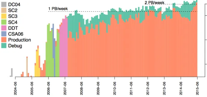
3.1) make possible a wide set of actions, e.g. transfer subscription, monitoring of the transfer progresses and latencies, health controls of the software agents, etc... Originally PhEDEx was designed to perform transfers of massive volumes of data among WLCG computing. During Run-1 PhEDEx moved 150 PB and currently it is moving about 2.5 PB of data per week among 60 sites (Figure 3.2 and 3.3) [Cap 1, 38].

While the desired level of throughput has been successfully achieved, it is still common to observe transfer workflows that not reach full completion in a timely

(34)

24 CHAPTER 3. REDUCING LATENCIES IN CMS TRANSFERS

Figure 3.2: Overall data volume moved by PhEDEx since 2004. Note the logarithmic scale.

Figure 3.3: Cumulative transfer volume managed by PhEDEx among all Tiers in a 30 days period around September 2015. Each color represent a Tier-X to Tier-Y connection. Lower data volumes are even hardly visible as the total of active links is more then 2650.

(35)

3.1. CAN PHEDEX BE IMPROVED? 25 manner due to a small fraction of stuck files that require manual intervention. This chapter will provide a general view of the latency issue in CMS transfers while actual analysis will be addressed in Chapter 4.

3.1 Can PhEDEx be improved?

The PhEDEx design aims at providing the highest possible transfer completion rate, although possible infrastructural unreliabilities, through fail-over tactics and automatic retrial. This particular choice however does not minimize the waiting time of individual users for the completion of their jobs.

For this reason, during several years of operations, a large set of data concerning latencies observed in all transfers between Tiers has been collected: their study allows a categorization of such latencies in order to attack them appropriately at the development level so to ultimately improve the system and increase its overall preformances.

3.1.1 Instrumenting PhEDEx to collect latency data

Data produced from the CMS experiment are collected into datasets which regroup similar physical information coming from particle collisions e.g. the final state of 4 muons events. Nevertheless the atomic unit for transfer operations in PhEDEx is the file block: an arbitrary group of O(100-1000) files in the same dataset. Initially all information were block-level organized and PhEDEx didn’t record states of individual files: for this particular reason, in 2012, this system was instrumented to detect latency issues with historical monitoring tables, containing file-level informations, and equipped with useful tools to retrieve monitoring data for further analysis.

The first agent, called BlockAllocator, that is responsible for monitoring subscrip-tions, records the timestamps of the main events related to block completion i.e. the time when the block was subscribed and the time when the last file in the block was replicated at destination. The difference between these timestamps can be defined as the total latency for the entire block as experienced by users including manual intervention.

The second agent, called FilePump, that is responsible for collecting the results of transfer tasks, records a summary of each file history inside the block such as the time when the file was first activated for routing or the number of transfer attempts needed for the file to arrive at destination, as well as the source node of the first and last transfer attempts.

For performance reasons, after the transfer is complete, these live tables are stored into historical log tables: file-level statistics in t_log_file_latency (usually deleted after 30 days) and block-level statistics into t_log_block_latency (permanently recorded) [Cap 2,38]. Those tables are integrated with additional events related to block completion such as:

• the time when the first file was routed for transfer;

(36)

26 CHAPTER 3. REDUCING LATENCIES IN CMS TRANSFERS • the time when 25%/50%/75%/95% of the files inside the block were replicated

at destination;

• the time when the last file of the block was successfully replicated at destina-tion;

• the total number of attempts needed to transfer all files in the block; • the source node for the majority of files in the block.

3.1.2 Cleaning data for latency analysis

Since 2012 the total amount of records collected about latencies has reached about 3 million block subscriptions. However before starting the analytics work presented in Chapter 4, this set of data has been cleaned and processed in order to remove uninteresting data and define useful observables. First of all there are ill data, i.e. records with missing or inconsistent data, mostly issued from test transfers and representing only the 5% of the total amount. There are also about 780000 that took place in blocks still open and growing in size. Furthermore 62000 transfer entries which have been suspended during their execution: these particular entries were removed because their treatment may render the whole process uselessly complex although being well-defined targets. It has been defined also a cutoff of 3 hours on the transfer time: seen the typical time scale of data transfers at CMS, if a transfer takes less than 3 hours from subscription to the completion we can, arbitrarily but sensibly, argue that it is not a candidate for having latency problems [Cap 3, 38]. Roughly 960000 items has been removed by this cutoff.

Although the total amount of subscriptions was nearly about 3 million, this cleaning procedure has allowed to remove about 2 million transfers, leaving a cleaner yet enough populated sample.

3.1.3 The "skew" variables

In order to determine the evidence of a latency effect, new variables have been introduced called "skew" variables. These variables show the transfer rate ratio between a small portion of time (such as the last 5% or the first 25%) and the X percent from the beginning or to the end of a transfer.

More precisely:

• Skew x variables:

SkewX = transfer rate of the

LAST 5 percent of the files transfer rate of the FIRST X percent of the files ·

X

5 (3.1) where X = 25, 50, 75, 95;

• Skew Last X variables:

SkewLastX = transfer rate of the LAST 5 percent of the files transfer rate of the LAST X percent of the files ·

X

5 (3.2) where X = 25, 50, 75;

(37)

3.1. CAN PHEDEX BE IMPROVED? 27 • Reverse Skew X variables:

RSkewX =

transfer rate of the FIRST 25 percent of the files transfer rate of the FIRST X percent of the files ·

X

25 (3.3) where X = 50, 75, 95;

• Reverse Skew Last X variables: RSkewLastX = transfer rate of the

FIRST 25 percent of the files transfer rate of the LAST X percent of the files ·

X

25 (3.4) where X = 5, 25, 50, 75.

On a transfer ideally running at a constant rate all these variable would have value 1. Skew variables that significantly differs from unity can be considered a good hint of a transfer with latency issues. These considerations have led to a further data cleaning: only block with more than 5 files, a size larger than 300 GB and defined values for all the "skew" variables were left, being big enough to have a "bulk" and a "tail" [Cap 3, 38].

The analysis presented in Chapter 4 has been performed using roughly 42000 transfers entries which are the result of this skimming process.

3.1.4 Types of latency

Transfers may be affected by latency issues in different ways. In this work, attention has been put on these particular types of latency: late stuck (already referred to as transfer "tail") and early stuck.

Late Stuck

Late stuck files are present when one or few files take much longer to get transferred than the rest of the block. In figure3.4, sample plots of the number of files at destination as a function of time are shown. Different patterns and temporal scales in block completion are clearly visible [47]. Figure 4.32a shows a normal transfer trend: in this scenario, block completion is gradual from its subscription until the end in a reasonable time. Figure 4.32b, instead, shows a transfer with a final "tail": unlike the previous image, the last 5% (in red) requires a longer time than the rest of the block to complete, and probably only a manual intervention allowed its actual completion.

This type of latency can be observed by selecting transfers in which the time needed for moving the last 5% of bytes is larger than a given threshold δ. To prevent very large blocks from being included even if they have no real latency issues we may add to δ an offset which depends from the size of the block and a reference speed parameter v. In formulas

∆Tlast5% > δ + S

20v (3.5)

where ∆Tlast5% is the time of the last 5% of replicas and S the size of the block. Sensible values used for the parameters are v = 5MB/s and δ = 10h [Cap 4,38]. The CMS data production and processing tasks over WLCG may occasionally

(38)

28 CHAPTER 3. REDUCING LATENCIES IN CMS TRANSFERS

(a) Percentage of files at destination as a function of time since subscription, for a block transferred with perfect transfer quality

(b) Percentage of files at destination as a function of time since subscrip-tion, for a block with a few perma-nently stuck files ("transfer tail")

Figure 3.4: Comparison between a block with perfect transfer quality (a) and a block with stuck files (b). More details on the differences among the two plot, in particular the red segment, are presented in the text below.

produce corrupted outputs. This happens when one or a few files in a datablock are missing or resulting from a non-handled failure during storage or they have wrong size/checksum. PhEDEx has been designed to deal with such data corruption events and is able to detect them (thanks to internal checking mechanisms and pre/post validation scripts) and tag the corresponding transfers as failing. Moreover PhEDEx tries to minimize the impact of the corrupted files on the data placement operations by re-queuing them while it keeps on transferring the rest of the data. As the transfers of the corrupted files keep on failing systematically, PhEDEx suspends them for a longer time and creating consequently a transfer "tail".

Reasons of such latency are heterogeneous but mostly due to storage problems, which explains why only a few files are affected from this issue. These late stuck can have a very important impact on CMS operations: in fact, transferred data is often useless to CMS analysts until its completion. Therefore it is quite important to find the stuck files and fix the underlying problem as soon as possible. Usually a manual intervention is required, consisting of either replacing the file or, if there is not any uncorrupted data, announcing it as lost [Cap 5,38].

Among other analysis, chapter 4 will provide a study of these tails, showing the impact of these missing/corrupt files clearly visible at the last few percentages of the whole block transfer.

Early Stuck

Early stuck latency affects those blocks that begin with serious performance issues and start flowing properly only after some time, presumably once such issues have been fixed.

This type of latency can be observed by selecting transfers in which the time for the first replica is larger than a given threshold δ. To prevent very large blocks from being included even if they have no real latency issues we may add to δ an offset which depends from the average size of the files and the reference rate parameter v.

(39)

3.1. CAN PHEDEX BE IMPROVED? 29 In formulas

∆T1st> δ + hSi

v (3.6)

where ∆T1st is the time of the first replica and hSi the size in the datablock. The same values of v and δ shown above can be used [Cap 4,38].

Early stuck situation, if not promptly identified, leads to serious consequences: only a quick problem identification, attach and fix can avoid to pile up delays and additional work load [Cap 4, 38]. The solution for this latency is not straight-forward: it may require admin intervention at the source or destination site, or even an involvement by central operators.

(40)

(41)

Chapter 4 Analysis of latency data

In this chapter the analysis made to investigate the PhEDEx performances will be described. Studying this data has allowed to observe different patterns and trends depending on the type of latency that we have previously introduced and described (see Section 3.1.4). In particular, the definitions used for the different latency types (see eq. 3.5 and3.6) represent the starting point of the entire analysis. Such definitions have been discussed and decided within a group of PhEDEx developers and operators with we started a collaboration, and also contributed together with a paper presented at the Conference on Computing for High Energy Physics 2015 (CHEP 2015)[38]).

The goal of our analysis is manifold: in the first place we want to verify if the definitions stated above are well suited to select samples with a certain degree of purity; secondly, we want to identify characteristic markers that reduce the variability and hence suggest either real-time monitoring action to be adopted by PhEDEx developers (e.g. new features, code improvements or refinements).

4.1 Data collection and elaboration

Initially data were collected inside a .csv file of enormous dimensions produced by the PhEDEx monitoring system (described in detail in Section 3.1.1) that required a lot of time in order to be compiled and executed. After an optimization work, this .csv file has been reduced to roughly 3 million entries (skimmed using the procedure described in Section 3.1.2) and information were better organized. We elaborated these data interactively using a R1 _{script through an user interface} called RStudio [48] (see Figure 4.1): using my laptop the compilation time required about half an hour.

Plots and histograms produced have been divided depending on the latency type i.e. Early Stuck and Late Stuck. At last, for the sake of clarity, another particular type of latency called "Stuck Other", untreated in Chapter 3, will be briefly explained.

Initially we noticed a particularity in the definition of the latencies typologies: 1_{R is a GNU programming language and software environment for statistical computing and}

graphics created by Ross Ihaka and Robert Gentleman at the University of Auckland.

(42)

32 CHAPTER 4. ANALYSIS OF LATENCY DATA

Figure 4.1: RStudio user interface [48] used for the analysis of the .csv file produced by PhEDEx.

they are not independent i.e. some overlap exists between them. Table4.1shows an interesting detail: the sum of the three categories is greater than the sample itself; this implies a double-counting of some entries or rather a correlation between differ-ent latency typologies. In fact, looking at Table4.2we can notice (in red) an overlap of stuckLate latencies in the stuckEarly subset (about 10% of double-counting). So far, we have considered these categories as independent for the time being, in order to quickly attack the problem and gain more insight. We acknowledge this may not be optimal, and we foresee to expand the analysis in the near future.

In the next session, we will present the analysis and discuss key points of the Early Stuck and Late Stuck, separately.

Table 4.1: Count of the different typologies of latencies (stuckEarly, stuckLate, stuckOther). csvData represent the entire sample, data represent the sample after the skimming process, see text for more detail.

4.2 Early Stuck Analysis

The Early Stuck kind of latency - defined in Section3.1.4 - affects those blocks whose transfer begins with serious performance issues and start flowing properly

(43)

4.2. EARLY STUCK ANALYSIS 33

Table 4.2: Overlap between stuckEarly, stuckLate, stuckOther.

only after some time.

A typical trend of a block with Early Stuck issues is shown in Figure4.2: we can notice from the axis scales, that the first 25% in fact has a transfer rate of about 5 orders of magnitude smaller than the last 25%. Despite this plot seems obvious and easy to understand, it was never done before and may offer some useful information to PhEDEx operators when a transfer presents itself as an Early Stuck; having a chance to produce this plot in real time during CMS data transfers would allow to spot and promptly address data subscriptions that show illness since the very beginning, thus allowing PhEDEx operators to intervene and fix.

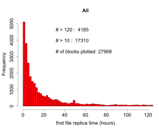
Another aspect to investigate in detail is shown in Figure 4.3: this histogram shows the time for the first file replica to appear at destination starting from the time when the subscription was inserted. We can notice a decreasing smooth trend with a maximum in the first hours, as expected.

However there are some particularities:

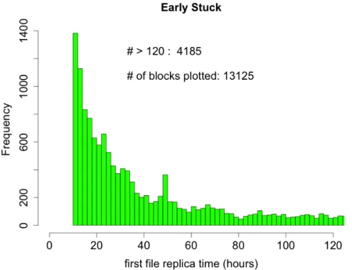
• using as lower limit for Early Stuck latencies δ = 10h in 3.6(see Figure4.4 to observe the cutoff) we assume as "problematic" nearly the 54% of the sample meaning that this type is predominant compared to the other stuck. This fact represent a problem because, if verified by further studies, means that latency issues for half the time occur at the very beginning of the transfer process thus making monitoring plots strongly recommended;

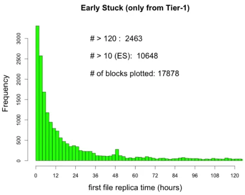
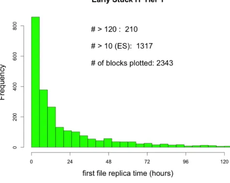
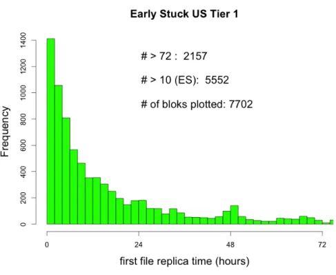
• there is a peak clearly visible in the 48h time interval (see Figure 4.5). This 48h peak originally made us presume that it was mainly due to Tier-2 centers: in fact, differently from Tier 1 sites, they do not work 24h/7 but only 8h/5 and e.g. a problematic subscription with latency issues made on Friday afternoon may not be solved until Monday morning causing a peak at roughly 48 hours. Instead Figure 4.6 and Figure 4.7 shows quite the opposite i.e. the 2 days peak is caused by Tiers 1. A plausible explanation of this phenomenon must be sought on the storage mechanisms of a Tier 1: custodial data, in fact, are stored on tapes that may require a tape robot related delay in order to retrieve the particular one that hosts the data requested for transfer. These delays apparently accumulate in a temporal windows of 48h, and create the peak as of Figure 4.6.

Another aspect to investigate in detail is shown in Figure 4.8: this plot shows a zoom on the first 24 hours in the transfer of the first file replica in a block. Each bin represent 1 hour, i.e. collects all the blocks whose transfer starts within 1

(44)

34 CHAPTER 4. ANALYSIS OF LATENCY DATA hour. A smooth behavior for increasing values of the first file replica time can be observed, with the exception of the increasing second bin which is analyzed in detail on Figure4.9: this plot shows an increasing trend until the maximum located at about 30 minutes from job subscription. This is an indirect measurement of the actual PhEDEx infrastructure latency in starting a transfer task: the transfer are managed by the specific "FileDownload" software agent, which is stateless and queries the PhEDEx TMDB (see Section 2.4) to get information on the work to be done. These agents have a default cycle of roughly 20 minutes before rechecking and reactivating themselves, which means that it is highly probable that within subscription and the first file replica a time larger than 1 hour passes, explaining the behavior we indeed observe.

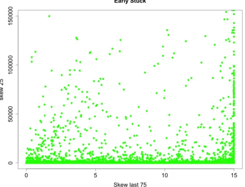
In Chapter 3, Section 3.1.3, we have introduced the "skew" variables: unlike the variables used for the previous investigations, these are by far more versa-tile and allow a wider scale latency investigation, but at the cost of sacrifying the simplicity of understanding and a certain level of intuitiveness. Many are the possible combination of these variables but not every single one of them is important to our goal: we have selected two of the most significant ones, and a bidimensional plot is shown in Figure4.10: this plot shows SkewLast75 vs Skew25 in transfers with Early Stuck latency. Recalling equations3.1 and3.2 the explanation is quite simple: files in the block are initially stuck causing a low first 25% rate and producing high values of Skew25 (according to eq. 3.1), however the remain-ing 75% is quite fast which produces low values of SkewLast75 (accordremain-ing to eq. 3.2). As data transfers having a given class of sites as sources and/or destination, as well as sources/destination being in specific nations may be affected by specific issues, a more in-depth analysis was performed in two directions: the first aimed at selecting only CMS Tier 1 (Tier 2) as source sites; the second aimed at distinguish-ing the transfers comdistinguish-ing from the same Tier level but in different nations. Both investigations, separately, are presented and the results discussed in the following paragraphs.

Tier 1 as sources

We already introduced the Figure 4.6 which we now discuss further. The trend is quite smooth, with no exception, decreasing from a maximum at just few hours. It is indeed known that in most cases a T1 outbound transfer should start quickly for several reason (for more detail of Tier 1 facilities see Section2.1.1). First a Tier 1 has plenty of tape server/drives resources, so actions may happen fluidly in parallel. Secondly a delay in exporting a file may come from the lack of a commissioned source-destination link, which is very rare for a Tier 1 as all outbound links have commissioned in advance.

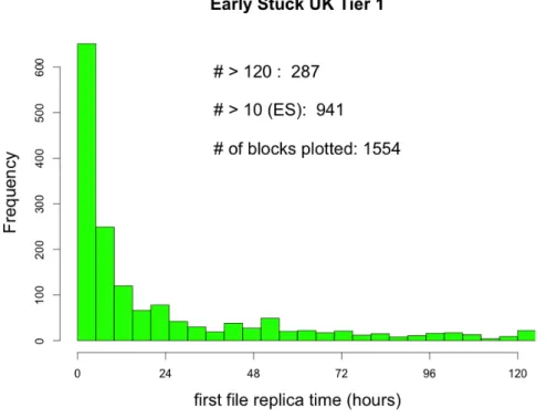
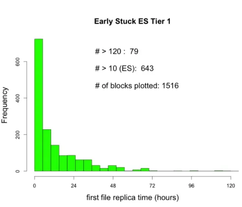
A further investigation was made by separating the different Tier 1 by nation: the results are displayed in Figure4.11 (Italian Tier 1),4.12 and4.13 (American Tier 1), 4.14 (German Tier 1), 4.15 (British Tier 1), 4.16 (French Tier 1), 4.17

(45)

Figure 4.2: Transfer rate of the first 25% of the block vs rate of the last 25% for transfers suffering from a latency of the Early Stuck type according to eq. 3.6.

(46)

Figure 4.4: Time for the first file replica at the destination site for Early Stuck transfer (with more than 10h waiting time).

(47)

Figure 4.6: Time for the first file replica to appear at the destination site, when the source site is a Tier 1.

Figure 4.7: Time for the first file replica to appear at the destination site, when the source site is a Tier 2.

(48)

Figure 4.8: First day zoom for the transfer of the first file replica at the destination site, for all data in the .csv file.

Figure 4.9: First 5 hours zoom for the transfer of the first file replica at the destination site, for all data in the .csv file.

(49)

Figure 4.10: Skew25 vs SkewLast75 as defined in eq. 3.1 and3.2, for transfers tagged as being Early Stuck according to eq. 3.6.

the PhEDEx site "T1_CH_CERN" (see Section2.1.1) as it is collocated with the Tier 0 and it is definitely a peculiar Tier 1 site, making a direct comparison with other off-CERN national centers not appropriate. Some comments specific to each are provided in the following:

1. Italian Tier 1 (Figure 4.11): smooth curve as expected with no particular exceptions;

2. American Tier 1 (Figure 4.12 and 4.13): larger data traffic (as known, as the US Tier 1 alone is about 40% of the CMS Tier 1 resources), smooth curve as expected with a massive initial activity (depicted in detail in the 3-day zoom plot);

3. German Tier 1 (Figure 4.14): smooth curve as expected as the US and IT trend;

4. British Tier 1 (Figure4.15): smooth curve with a slight final increase probably caused by some some tendency to accumulate backlog (a further analysis would be needed to understand if this is related to their specific storage solution, and this goes beyond the scope of this thesis);

5. French Tier 1 (Figure 4.16): smooth curve as expected, but exporting a definitely smaller data volume ;

6. Spanish Tier 1 (Figure 4.17): same considerations as the French Tier 1. Table 4.3, at last, shows the fraction of Early Stuck entries divided by nation from Tier 1 sources.

(50)

Figure 4.11: Time for the first file replica from IT Tier 1 source.

(51)

Figure 4.13: Time for the first file replica from US Tier 1 source (3-day zoom).

(52)

Figure 4.15: Time for the first file replica from UK Tier 1 source.

(53)

Figure 4.17: Time for the first file replica from ES Tier 1 source.

Table 4.3: Fraction of early stuck files and relative percentage for Tier 1 divided by nation.

(54)

44 CHAPTER 4. ANALYSIS OF LATENCY DATA Tier 2 as sources

We already introduced the Figure4.7which we now discuss further. While Tiers 1 are only 8 all around the world, Tiers 2 are more than 50 with quite a spread in location, size, service quality and performances. The most important thing is that within the first 2 days, most transfers just start, and only the queues remain to be dealt with. Nevertheless the curve showed in Figure 4.7 cannot be so relevant as it was for the Tiers 1.

For this reason, the corresponding results are shown on a more detailed study for each nation of interest (Figures 4.18, 4.19, 4.20, 4.21, 4.22, 4.23, 4.25,4.26). Table 4.4 shows the fraction of early stuck entries divided by nation from Tier 2 sources. An individual analysis is not necessary being very similar from each other. However some plots (RU Tier 2 4.19, US Tier 2 4.20, UK Tier 2 4.21) show a singular peak in the 72 hours area: this might be the convolution of the 48h scenario previously stated probably caused by a mix of time zone and human response.

Figure 4.18: Time for the first file replica from IT Tier 2 sources.

4.3 Late Stuck analysis

This other kind of latency has already been defined in Section3.1.4: it happens when one or few files take much longer to get transferred than the rest of the block. Figure 4.27 represent the typical trend of a block with a late stuck latency. The first 95% of the block, in fact, is transferred with a rate that is roughly 3 order of magnitude higher than the last 5%. In principle, if the transfer rate were flat, one would expect to see a bisector line.

(55)

4.3. LATE STUCK ANALYSIS 45

Figure 4.19: Time for the first file replica from RU Tier 2 sources.

(56)

Figure 4.21: Time for the first file replica from UK Tier 2 sources.

(57)

4.3. LATE STUCK ANALYSIS 47

Figure 4.23: Time for the first file replica from FR Tier 2 sources.

(58)

Figure 4.25: Time for the first file replica from CH Tier 2 sources.

Investigation of petabyte-scale data transfer performances with PhEDEx for the CMS experiment

Alma Mater Studiorum · Università di Bologna