Performance Analysis
and Numerical Results
5.1. Cramer-Rao Bound
In order to understand the theoretical limit on RSTD estimation, the Cramer-Rao Bound (CRB) is computed. The CRB represents the minimum achievable mean square error (MSE) for an unbiased estimator (the MSE is the variance for an unbiased estimator). As shown in chapter 4, the proposed estimator without channel estimation is biased and, even if the bias compensation is applied, a residual bias can still remain due to channel estimation error. Clearly, if the estimator is biased, its MSE performance cannot reach the CRB. Anyway, the CRB is useful to see what is the gap between the performance of the proposed estimator and best achievable performance. As mentioned in chapter 4, the UE knows the PRS timing of the reference cell after having received the OTDOA assistance data and, hence, in order to perform a RSTD estimation it has to measure the time of arrival of PRSs transmitted by a neighbour cell. For this reason, the RSTD estimation error (considering one PRS occasion), corresponds to the time of arrival estimation error, as shown in the following expression:
85 ̂
( ̂ ) ( ) ̂
where is the RSTD error, is the time of arrival error, ̂ is the estimated RSTD for the oth PRS occasion, is the correct RSTD value, ̂ is the estimated time of arrival of PRSs transmitted by the neighbour
cell c, is the correct time of arrival of PRSs transmitted by the neighbour
cell c and is the correct time of arrival of PRSs transmitted by the reference cell. Since , we will compute the CRB for the time of arrival estimation. For the CRB computation, we will consider a time-invariant multipath channel experienced by the transmitted signal, in the realistic case where the UE does not have any a priori knowledge of the channel. We compute the CRB considering the RSTD estimation performed after 1 PRS occasion.
The transmitted OFDM baseband signal can be expressed as:
∑ ∑
where is the kth subcarrier frequency, { }, is the number of used subcarriers (e.g. for 10 MHz bandwidth the DFT size is N=1024, but only =600 subcarriers are used), is the number of PRS OFDM symbols within an occasion, is the OFDM symbol duration, is the set of subcarriers used for PRS transmission within the th PRS OFDM symbol ( subcarriers), is the time domain pulse with energy and is the QPSK PRS modulation symbol transmitted on the kth subcarrier within the th PRS OFDM symbol. The use of the CP is assumed [18].
86
The power of the transmitted baseband signal is
where /6 is the number of subcarriers used for PRS transmission for one OFDM symbol, according to the PRS mapping (see chapter 3).
Assuming the subcarrier spacing =1/T is smaller than the channel coherence bandwidth (as mentioned in chapter 4, this approximately means < 10.6 ms), so that each subcarrier experiences a flat frequency domain channel, the received baseband signal in the case of absence of interference can be modeled as [18]:
with ∑ ∑
where is the propagation delay, is complex AWGN with power spectral density for each component and is the complex channel coefficient at frequency . approximately represents the delay of the shortest path (in particular, this approximation is quite accurate in the presence of the LOS), hence the time of arrival to be estimated. The UE has to estimate from the observation of , assuming a sufficiently long observation interval such that comprises the whole received signal.
Considering the generic th
OFDM symbol, the power of the received baseband signal is ∑ | | , hence it depends on the complex channel coefficients at
87
the equal-spaced subcarriers frequencies where PRSs are transmitted. Assuming a normalized channel frequency response (∑ | | ), considering that, in general, some subcarriers are attenuated (| | <1) and other subcarriers are amplified (| | >1), we can approximate the power of the received baseband signal as
.
The Fourier transform of is:
∑ ∑
where is the Fourier transform of the pulse . The received signal depends on
the unknown channel parameters that are collected in a (2 +1)-length vector
defined as follows:
[ ] where and are -length vectors collecting amplitudes and phases of the complex channel coefficients at subcarriers used respectively:
[
]
[
]
Let us define a U-dimensional vector containing the indexes of the subcarriers used for PRS transmission among all PRS OFDM symbols:
88
We will use the following notation to refer to channel parameters at subcarriers used for PRS transmission:
where is the kth element of , with 1 ≤ k ≤ U. Then, we define
as the PRS OFDM symbols that use the subcarrier frequency and as the PRS OFDM symbols that use the subcarrier frequency .
The CRB is computed as [18]:
[ ]
where is the (2 +1) x (2 +1) Fisher information matrix, whose element on the
roth row and the coth column (1 ≤ ro, co ≤ 2 +1) is [18]: [ ] { ∫ }
89
where is the roth element of and is the partial derivative of with respect to computed for the effective values of the elements of
corresponding to the experienced channel. We use { } to denote the real part of and { } to denote the imaginary part of .
From and , after some analytical computations, it is possible to find that the Fisher information matrix can be written as:
[
]
where is the transpose of M. The Fisher information matrix is formed by six elements: is a scalar defined as
{∑ ∑ ∑ ∑ }
and are two 1 x vectors whose cth elements (1 ≤ c ≤ ) are
[ ] { ∑ ∑ ∑ } [ ] { ∑ ∑ ∑ }
90
, and are three x matrixes whose elements on the rth row and the cth
column (1 ≤ r, c ≤ ) are [ ] { ∑ ∑ } [ ] { ∑ ∑ } [ ] { ∑ ∑ } with ∫ ∫ ∫
91
for q=0, 1, 2. We can observe that , is the skewness of the spectrum | | and is the mean-squared bandwidth of [18].
Assuming that is the unique unknown parameter while the other channel parameters are known, the CRB is (this approach is called conditional bounding [18]).
Considering the time domain pulse , whose Fourier transform is , the bandwidth of the transmitted signal is infinite, resulting in a unrealistic case. In this case we can easily verify that can be theoretically estimated without error, since the CRB tend to zero (the mean-squared bandwidth tend to infinity). In order to have a finite bandwidth signal, we approximate with its main lobe that carries the main part of the energy of the signal (a value of about 90.3% of the total energy can be found numerically). With this approximation, i.e. , the two-sided bandwidth of the baseband signal is ( +2)/T. Introducing this approximation and, in general, if a finite bandwidth is considered, the theoretical orthogonality among subcarriers is lost, i.e. .
After some analytical computations, we can find the following expressions for the integrals :
| |
{ [ ] [ ]
92 { [ ] [ ] [ ]} { [ ] [ ] [ ]} { [ ] [ ] [ ]} { [ ] [ ] [ ]} { { [| |] [| |] [| |]} { } { [ ] [ ] [ ]}
93 { [ ] [ ] [ ]} where { | |
and are the sine integral and cosine integral functions defined as [19]
∫ and ∫ is [19]
94
with the natural logarithm of and the Euler-Mascheroni constant ( = 0.5772156…). The resolution of the integrals leads to integrals of functions with singular points within the integration interval. In order to find a solution of these ill-defined integrals, the Cauchy principal value has been considered [19].
5.2. Estimation Performance
5.2.1. General Assumptions
We consider the bandwidth B=10 MHz with a sampling frequency =15.36 MHz ( =1/ 65.1 ns), corresponding to N=1024, =72, =600 and U=500. We consider a scenario with three cells, one reference cell and two neighbour cells, whose configuration parameters are shown in table 5.1. The parameters of the cells have been chosen such that: PRSs are effectively transmitted, since they are not mapped into REs reserved for PBCH, PSS and SSS (see sections 1.3.4 and 1.3.5); PRSs of different cells are not overlapping, avoiding inter-cell interference. Considering different PRS configuration indexes, the PRS time differences of arrival contain also time offsets due to different PRS transmission times of the cells. The UE can measure the RSTDs without these time offsets because it knows the PRS configuration indexes received within the OTDOA assistance data. For each neighbour cell, we consider the maximum search window size according to the LPP [10], i.e. =3069 samples ( 0.2 ms). This means that the number of steps considered within the search window during the coarse timing is ⌈ ⌉=43. Considering that the fine timing
resolution (maximum timing error that can be estimated) is N/2=512 samples (see section 4.3.2), we can conclude that the coarse timing step is required.
95
Tab. 5.1 – Cells configuration parameters.
reference cell neighbour cell 1 neighbour cell 2 physical layer cell
identity 0 1 2
2 7 18
1 1 1
PRS muting
sequence 1111111111111111 1111111111111111 1111111111111111 search window size - 3069 samples ( 0.2 ms) 3069 samples ( 0.2 ms)
RSTD - 56 samples ( 3.65 µs) ( 5.73 µs) 88 samples
We consider the AWGN scenario and multipath channel scenarios in the cases of time-invariant channel and time-variant channel. In the ideal case of AWGN, since there is no multipath channel, we will not consider the bias compensation. The numerical results are obtained by averaging over 100 independent channel realizations where the RSTD estimation is performed after 16 PRS occasions and by averaging 1600 independent channel realizations where the RSTD estimation is performed after 1 PRS occasion. The results have been obtained using the Intel® Matlab LTE-A Link Level Simulator.
In a real scenario, the RSTD measurements are affected by different types of error. The main sources of error are [13]: eNodeBs synchronization error; UE frequency instability; RSTD measurement quantization error; estimator error; multipath propagation error. The simulations have been performed assuming that the first two errors do not occur. Furthermore, we have considered RSTD values that are multiples of the sampling time, avoiding the quantization error. We will consider the last two types of error that are those affecting more heavily the estimation.
96
5.2.2. Numerical Results
We will show results about one RSTD estimation, hence considering one of the two neighbour cells, since the two RSTD measurements are characterized by the same performances. The RSTD results are expressed in terms of the range difference error, which is computed as the RSTD error multiplied by the speed of light c. We will show performance of RSTD measurements using 1 PRS occasion and using 16 PRS occasions.
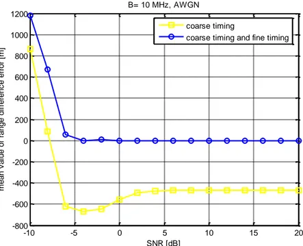
Firstly, we make a comparison between the coarse timing, i.e. the RSTD computed by means of the coarse timing step only, and the coarse timing plus the fine timing. Figure 5.1 shows the mean value of the range difference error for coarse timing and for coarse timing plus fine timing, in the case of AWGN. As we can easily understand, the mean value of the range difference error is the same for the cases of 1 and 16 PRS occasions, since the RSTD estimation using 16 PRS occasions consists of the average of the RSTD measures performed for each occasion.
We can observe that the coarse timing works for SNR> 4 dB, obtaining a mean error whose value is the minimum achievable one, due to the CP step size used. In particular, this minimum error (depending on the search window position and on the PRS time of arrival of the considered neighbor cell) is about 469 m, corresponding to a timing error of 24 samples (smaller than the CP length). After fine timing, the mean error is zero for SNR> -4 dB. The fine timing works also for small SNR values where the coarse timing performances are affected by the noise (the residual timing error after coarse timing can be bigger than the CP length). We note that the estimator is not biased, because of the absence of a multipath channel.
97
Fig. 5.1 – Mean value of range difference error using coarse timing and using coarse timing
plus fine timing (AWGN).
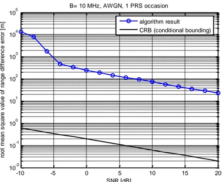
Still considering the AWGN case, let us compare the root mean square value of the range difference error (RMSE) for 1 PRS occasion with the maximum achievable performances represented by the CRB (figure 5.2). In the ideal AWGN case, since there is no multipath channel, the CRB has been computed following the conditional bounding approach, as in [13]. We can see that for SNR> -4 dB the RMSE obtained is parallel to the CRB, but with a big performance gap (the RMSE is about 1000 times bigger than the best achievable one). At a SNR value of 20 dB, the RMSE obtained is about 24 m. The algorithm performance does not reach the CRB because we have not considered the ML estimator [18]. Furthermore, it is important to note that the proposed algorithm uses six PRS OFDM symbols within a subframe, even if eight PRS OFDM symbols are available (see sections 4.3.1 and 4.3.2). The fact that only some of the all PRSs transmitted are use is another explanation for the gap between
-10 -5 0 5 10 15 20 -800 -600 -400 -200 0 200 400 600 800 1000 1200 SNR [dB] m e a n v a lu e o f ra n g e d if fe re n c e e rr o r [m ] B= 10 MHz, AWGN coarse timing
98
the algorithm performance and the CRB (computed considering all PRS OFDM symbols).
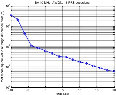
Figure 5.3 shows the RMSE in the case of 16 PRS occasions and AWGN. Averaging the estimates performed for each occasion, the RMSE is greatly reduced, obtaining a value of 6 m at SNR=20 dB.
Fig. 5.2 – Root mean square value of the range difference error for 1 PRS occasion and the
CRB (AWGN). -10 -5 0 5 10 15 20 10-2 10-1 100 101 102 103 104 105 SNR [dB] ro o t m e a n s q u a re v a lu e o f ra n g e d if fe re n c e e rr o r [m ] B= 10 MHz, AWGN, 1 PRS occasion algorithm result CRB (conditional bounding)
99
Fig. 5.3 – Root mean square value of the range difference error for 16 PRS occasion
(AWGN).
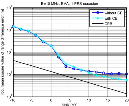
Let us consider a realistic scenario, that is the case of multipath channel. Figure 5.4 shows the RMSE obtained and the CRB in the case of 1 PRS occasion and EVA channel model. Two types of results are shown: the results obtained with the synchronization algorithm without bias compensation (without CE) and the results obtained with bias compensation (with CE). Without bias compensation, we can see that a floor exists due to the bias introduced by the multipath channel, resulting in a RMSE of about 100 m at SNR= 20 dB. After bias compensation the RMSE is reduced, but a floor still remains, due to the channel estimation error. For 4 dB ≤SNR≤ 12 dB, the RMSE curve is almost parallel to the CRB, with a performance gap of 8.5 dB in terms of SNR. For SNR values larger than 12 dB, the gap increases due to the floor. At SNR= 20 dB, RMSE 60 m.
-10 -5 0 5 10 15 20 100 101 102 103 104 SNR [dB] ro o t m e a n s q u a re v a lu e o f ra n g e d if fe re n c e e rr o r [m ] B= 10 MHz, AWGN, 16 PRS occasions
100
Fig. 5.4 – Root mean square value of the range difference error for 1 PRS occasion and the
CRB (EVA).
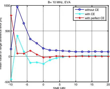
Figure 5.5 shows the mean value of the range difference error for EVA channel. This figure shows also results obtained with bias compensation in case perfect channel estimation is available (with perfect CE). We can observe that without bias compensation the estimator is biased due to the multipath channel, resulting in a mean error of about 90 m for SNR> 6 dB. If bias compensation is performed, the bias is greatly reduced. The channel estimation works from a sufficiently high SNR value, namely about 6 dB, obtaining an almost constant and small mean error. However, even at lower SNR values, the channel estimation improves performances. At SNR= 20 dB, the mean error is about 10 m. In the case of perfect channel estimation, the bias is almost compensated, obtaining a mean error of about 3 m at SNR=20 dB. The small residual bias that still remains also after perfect channel estimation is due to the fact that bias compensation is based on the approximated relation between the timing error caused by the multipath channel and the CPDG parameter (see section 4.4).
-10 -5 0 5 10 15 20 101 102 103 104 105 SNR [dB] ro o t m e a n s q u a re v a lu e o f ra n g e d if fe re n c e e rr o r [m ] B=10 MHz, EVA, 1 PRS occasion without CE with CE CRB
101
Fig. 5.5 – Mean value of range difference error (EVA).
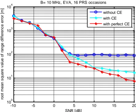
Figure 5.6 shows the RMSE obtained considering 16 PRS occasions. We can see that without bias compensation a clear floor appears, resulting in a RMSE of about 90 m for SNR≥ 6 dB. With CE the performance are greatly improved (RMSE 17 m at SNR= 20 dB), but a floor still remains. If perfect channel estimation is performed, the bias is almost compensated and the floor does not appear anymore. At SNR= 20 dB, the RMSE is about 7.5 m.
-10 -5 0 5 10 15 20 -500 0 500 1000 SNR [dB] B= 10 MHz, EVA m e a n v a lu e o f ra n g e d if fe re n c e e rr o r [m ] without CE with CE with perfect CE
102
Fig. 5.6 – Root mean square value of the range difference error for 16 PRS occasions (EVA).
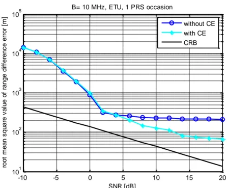
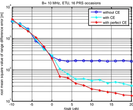
Figures 5.7, 5.8 and 5.9 show the results of the three previous figures for ETU, a more frequency selective channel model. As we can see from figure 5.7, a floor occurs in the case without bias compensation, resulting in a RMSE of about 220 m at SNR= 20 dB. This RMSE value is bigger than the correspondent RMSE value obtained for EVA channel because of the bigger bias introduced by the ETU channel. With bias compensation, although a floor remains, the RMSE is reduced. For 4 dB ≤SNR≤ 8 dB, the RMSE curve is almost parallel to the CRB, with a performance gap of 8.5 dB in terms of SNR. For SNR values larger than 8 dB, the gap increases due to the floor. At SNR= 20 dB, RMSE 70 m. Figure 5.8 shows that at SNR= 20 dB the ME values are about 185 m, 27 m and 12 m for the cases without CE, with CE and with perfect CE respectively. From figure 5.9, at SNR= 20 dB, we can see a RMSE of about 190 m without bias compensation, while with bias compensation the RMSE value is reduced to 30 m and if perfect channel estimation is performed the value is further reduced to
-10 -5 0 5 10 15 20 100 101 102 103 104 SNR [dB] ro o t m e a n s q u a re v a lu e o f ra n g e d if fe re n c e e rr o r [m ] B= 10 MHz, EVA, 16 PRS occasions without CE with CE with perfect CE
103
15 m. We can observe that, considering the complete synchronization algorithm (with bias compensation), the performances are worse than the case of EVA. Also in the case of perfect channel estimation, the ETU performances are worse than the EVA performances. In particular, comparing figures 5.6 and 5.9, we can see that after perfect channel estimation for EVA the bias is almost compensated and the floor does not occur, while for ETU a floor still remains. In fact for ETU the first samples of the OFDM symbol of interest are affected by ISI, because the CIR duration is larger than the CP length: the CP length (not considering the first OFDM symbol of a slot) is about 4.7 µs (see section 1.3.1), while the ETU maximum excess tap delay is 5 µs (see table 4.1). As mentioned in section 4.4, in general, after the first fine timing step, due to the multipath channel and interference (considering a sufficiently high SNR value), the few first samples of the OFDM symbol of interest are lost and few samples of the next OFDM symbol are detected, leading to interference of an undesired OFDM symbol. The number of samples lost is usually bigger for ETU, because of the larger error caused by the more frequency selective channel, although, anyway, the number of samples lost is small (see section 4.4). For ETU, in addition, the CIR duration can be longer than the CP length plus the few first samples lost (whose number depends on the particular channel realization), hence the first detected samples can be affected by ISI. Applying the second fine timing step, the resulting bias is caused by the multipath channel and a consistent amount of ISI. If perfect channel estimation is performed, the channel effect is compensated, while the ISI effect still remains.
104
Fig. 5.7 – Root mean square value of the range difference error for 1 PRS occasion and the
CRB (ETU).
Fig. 5.8 – Mean value of range difference error (ETU).
-10 -5 0 5 10 15 20 101 102 103 104 105 SNR [dB] ro o t m e a n s q u a re v a lu e o f ra n g e d if fe re n c e e rr o r [m ] B= 10 MHz, ETU, 1 PRS occasion without CE with CE CRB -10 -5 0 5 10 15 20 -600 -400 -200 0 200 400 600 800 SNR [dB] m e a n v a lu e o f ra n g e d if fe re n c e e rr o r [m ] B= 10 MHz, ETU without CE with CE with perfect CE
105
Fig. 5.9 – Root mean square value of the range difference error for 16 PRS occasions (ETU).
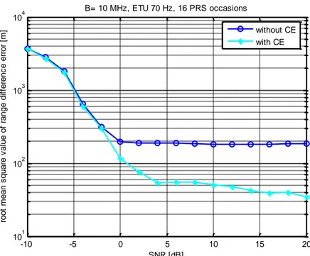
Now, we analyse the more realistic case of a time-variant channel, considering a maximum Doppler frequency of 70 Hz, that meets the assumptions made in section 4.3 when defining the synchronization algorithm ( ≤358.1 Hz). Figures 5.10 and 5.11 show the mean error and the RMSE for ETU channel with =70 Hz (ETU 70 Hz), considering 16 PRS occasions. We can see that this time-variant channel does not affect the algorithm performance, since we have results similar to those obtained considering a time-invariant channel.
-10 -5 0 5 10 15 20 101 102 103 104 SNR [dB] ro o t m e a n s q u a re v a lu e o f ra n g e d if fe re n c e e rr o r [m ] B= 10 MHz, ETU, 16 PRS occasions without CE with CE with perfect CE
106
Fig. 5.10 – Mean value of range difference error (ETU 70 Hz).
Fig. 5.11 – Root mean square value of the range difference error for 16 PRS occasions
(ETU 70 Hz). -10 -5 0 5 10 15 20 -200 0 200 400 600 800 1000 1200 1400 SNR [dB] m e a n v a lu e o f ra n g e d if fe re n c e e rr o r [m ] B= 10 MHz, ETU 70 Hz without CE with CE -10 -5 0 5 10 15 20 101 102 103 104 SNR [dB] ro o t m e a n s q u a re v a lu e o f ra n g e d if fe re n c e e rr o r [m ] B= 10 MHz, ETU 70 Hz, 16 PRS occasions without CE with CE
107
5.3. UE Localization Accuracy
5.3.1. General Assumptions
We will use the RSTD measurements obtained through the proposed synchronization algorithm applied to two neighbour cells to perform hyperbolic lateration and estimate the two-dimensional UE position. We will maintain the same assumptions made in section 5.2.1. In order to estimate the UE position, we need to know the positions of the base stations of the reference cell (base station 0) and the two neighbour cells (base stations 1 and 2). The assumed positions of the base stations and the position of the UE (depending on the base stations positions and the right RSTD values shown in table 5.1) are shown in figure 5.12. The aim is to show the UE localization accuracy in the explained scenario, as an example. In general, the performances depend on the particular geometric configuration of the base stations and the UE. The hyperbolic lateration will be performed using the Chan’s method which is a non iterative approach approximating of the ML estimator when the RSTD errors are small [20]. We will show result for the ideal case of AWGN and for the time-variant multipath channel ETU 70 Hz. We consider the RSTD measurements performed after 16 PRS occasions to compute the UE position.
108
Fig. 5.12 – Geometric configuration of the base stations and the UE.
5.3.2. Numerical Results
Figures 5.13 and 5.14 show the mean value and the standard deviation of the UE position error respectively for the AWGN case. Figure 5.15 shows the root mean square error that jointly describes the mean error and the standard deviation of the error. At SNR= 20 dB, we have an error with a mean value of about 10 m and with a standard deviation of about 3 m. The corresponding root mean square value of the UE position error is 10.5 m. -10 -5 0 5 10 -10 -5 0 5 10 X [Km] Y [ K m ] BS 0 BS 1 BS 2 UE BS 0: (2,4) BS 1: (-3,-3) BS 2: (10,-6) UE: (3.83,-1.58)
109
Fig. 5.13 – Mean value of the UE position error (AWGN).
Fig. 5.14 – Standard deviation of the UE position error (AWGN).
-10 -5 0 5 10 15 20 100 101 102 103 104 SNR [dB] m e a n v a lu e o f U E p o s it io n e rr o r [m ] B= 10 MHz, AWGN -10 -5 0 5 10 15 20 100 101 102 103 104 105 SNR [dB] s ta n d a rd d e v ia ti o n o f U E p o s it io n e rr o r [m ] B= 10 MHz, AWGN
110
Fig. 5.15 – Root mean square value of the UE position error (AWGN).
Figures 5.16, 5.17 and 5.18 show the results in the case of ETU. If the bias compensation is not performed, at SNR= 20 dB we have a mean error of about 143 m and a standard deviation of about 13 m, corresponding to a root mean square error of 144 m. Considering the bias compensation, the bias of the RSTD estimator is greatly reduced, obtaining a better UE localization accuracy for SNR≥ 0 dB. At SNR= 20 dB, we have a mean error of about 24 m and a standard deviation of about 8 m, corresponding to a root mean square error of 25 m.
-10 -5 0 5 10 15 20 101 102 103 104 105 SNR [dB] ro o t m e a n s q u a re v a lu e o f U E p o s it io n e rr o r [m ] B= 10 MHz, AWGN
111
Fig. 5.16 – Mean value of the UE position error (ETU).
Fig. 5.17 – Standard deviation of the UE position error (ETU).
-10 -5 0 5 10 15 20 101 102 103 104 SNR [dB] m e a n v a lu e o f U E p o s it io n e rr o r [m ] B= 10 MHz, ETU without CE with CE -10 -5 0 5 10 15 20 100 101 102 103 104 SNR [dB] s ta n d a rd d e v ia ti o n o f U E p o s it io n e rr o r [m ] B= 10 MHz, ETU without CE with CE
112
Fig. 5.18 – Root mean square value of the UE position error (ETU).
Figures 5.19, 5.20 and 5.21 show the results in the case of ETU 70 Hz. We can observe that these results are similar to those obtained considering a time-invariant channel. If the bias compensation is not performed, at SNR= 20 dB we have a mean error of about 147 m and a standard deviation of about 15 m, corresponding to a root mean square error of 148 m. Considering the bias compensation, at SNR= 20 dB, we have a mean error of about 27 m and a standard deviation of about 10 m, corresponding to a root men square error of 29 m.
-10 -5 0 5 10 15 20 101 102 103 104 SNR [dB] ro o t m e a n s q u a re v a lu e o f U E p o s it io n e rr o r [m ] B= 10 MHz, ETU without CE with CE
113
Fig. 5.19 – Mean value of the UE position error (ETU 70 Hz).
Fig. 5.20 – Standard deviation of the UE position error (ETU 70 Hz).
-10 -5 0 5 10 15 20 101 102 103 104 105 SNR [dB] m e a n v a lu e o f U E p o s it io n e rr o r [m ] B= 10 MHz, ETU 70 Hz without CE with CE -10 -5 0 5 10 15 20 100 101 102 103 104 105 106 SNR [dB] s ta n d a rd d e v ia ti o n o f U E p o s it io n e rr o r [m ] B= 10 MHz, ETU 70 Hz without CE with CE
114
Fig. 5.21 – Root mean square value of the UE position error (ETU 70 Hz).
-10 -5 0 5 10 15 20 101 102 103 104 105 106 SNR [dB] ro o t m e a n s q u a re v a lu e o f U E p o s it io n e rr o r [m ] B= 10 MHz, ETU 70 Hz without CE with CE