A cell-model for the multi-cell modelling of battery-packs

(1)

A Cell-Model for the Multi-Cell

Modelling of Battery-Packs

A Master’s Thesis

Academic Year: 2018/2019

Author: Angelo Cheli BSc

Student ID: 898323

(2)

ABSTRACT

Since modern society is so heavily reliant on internal combustion vehicles (ICVs), electric vehicles (EVs) have been one of the free market’s responses to their polluting nature. However, the major factor obstructing EVs from ubiquity is the inability of modern batteries to meet the energy and power requirements of ordinary cars for extended amounts of time. Because of this, not only are EVs generally much smaller than regular vehicles, but the energy stored in their batteries must be managed very carefully.

Measuring the energy left in the battery is impractical in automotive applications and must thus be estimated. To make this crucial estimation, the battery management system (BMS) relies on a model of the battery. The more accurate the model, the better the estimation and the more reliable the battery effectively becomes.

Even though an EV battery is made up of many smaller electrochemical cells, it is usually modelled with just a scaled-up model of a single cell. This practice is unable to account for distributed phenomena or mismatches between the cells. A simple way to address these aspects is to model each cell individually. Our original goal was to study how mismatches in the parameters of the cells caused some to deplete faster than others, but there were no electrical circuit models (ECMs) available in the literature that could be used as the building block of a multi-cell model. To address the deficiency, this paper modifies the Thévenin model (TM) — the most popular ECM — in such a way that it can represent the behaviour of individual cells residing in a network of cells.

One of the issues that will have to be addressed is the TM’s inability to autonomously remain within the cell’s interval of charge. In online applications the TM needs the external help of the BMS to do this, but in many offline applications — such as ours — the BMS is unavailable. The solution proposed by this work is a switching system that prevents the current of the cell's ECM from exiting/entering it when it is completely discharged/charged. The switching system allow the cell-model to regulate itself when interacting with cells in parallel or in series to it.

The switching system will be controlled by a nonlinear bulk capacitor that tracks the cell’s charge and models its zero-current steady-state behaviour without the need for a separate side-system. Like this, the model can monolithically represent a cell in a multi-cell context. This may not sound very innovative but it makes the model and its system of equations look as tidy as possible; an aspect that must be considered when planning to model multiple cells.

(3)

In the literature, TMs may sometimes be seen using linear bulk capacitors, but never nonlinear ones. This is either because the given application needs only to represent the linear section of the 𝑂𝐶𝑉 − 𝑆𝑜𝐶 characteristic, or simply because linear capacitors are readily available in the component libraries of simulators while nonlinear ones are not, and must be user-defined.

The parameter estimation that was run on the battery-pack of our test car yielded results reasonable enough to conclude that our nonlinear capacitor functions properly, and that substituting it for the charge-controlled voltage generator of the TM is indeed valid. Finally, the study of the simple case of two cells in parallel demonstrates that the switching system works as intended.

(4)

Dato che la società moderna dipende così fortemente dai veicoli a combustione interna, i veicoli elettrici sono diventati una delle risposte del libero mercato alla loro natura inquinante. Tuttavia, il principale fattore che ostacola i veicoli elettrici dall'ubiquità è l'incapacità delle batterie moderne di soddisfare i requisiti di energia e potenza delle auto ordinarie per lunghi periodi di tempo. Per questo motivo, non solo i veicoli elettrici in genere sono molto più piccoli dei normali veicoli, ma l'energia immagazzinata nelle loro batterie deve essere gestita con molta attenzione.

La misurazione dell'energia rimasta nella batteria non è pratica nelle applicazioni automobilistiche e deve quindi essere stimata. Per effettuare questa stima cruciale, il sistema di gestione della batteria si basa su un suo modello. Più il modello è accurato, migliore è la stima e più efficace diventa la batteria.

Sebbene una batteria EV sia composta da molte celle elettrochimiche più piccole, di solito è modellata da un modello di una singola cella in scala. Questa pratica non è in grado di tenere conto di fenomeni distribuiti o disallineamenti tra le celle. Un modo semplice per affrontare questi aspetti è modellizzare ogni cella singolarmente.

Il nostro obiettivo originale era studiare come i disallineamenti nei parametri delle celle facessero sì che alcune si esaurissero più velocemente di altre, ma non c'erano modelli circuitali disponibili in letteratura che potessero essere usati come monade di un modello multi-cella. Per affrontare la carenza, la tesi modifica il modello di Thévenin in modo tale da rappresentare il comportamento delle singole celle, collegate tra loro. Uno dei problemi che dovranno essere affrontati è l'incapacità del modello di Thévenin di rimanere autonomamente all'interno dell'intervallo di carica della cella che modellizza. Attualmente, il modello di Thévenin ha bisogno dell'aiuto esterno del BMS per farlo, che non è disponibile in molte applicazioni offline, come la nostra. La soluzione proposta da questo lavoro è un sistema di commutazione che impedisce alla corrente del modello della cella di uscire/entrare quando la cella è completamente scaricata / caricata. Il sistema di commutazione consente al modello della cella di regolarsi da solo quando interagisce con altre celle in parallelo o in serie ad esso.

Il sistema di commutazione verrà controllato da un condensatore di massa non lineare che traccia la carica della cella e modellizza il suo comportamento stazionario a corrente nulla senza la necessità di un sistema separato. In questo modo, il modello può rappresentare, in modo monolitico, una cella in un contesto multi-cella. Questo potrebbe non sembrare molto innovativo, ma rende il modello il più ordinato possibile, così come il suo sistema di equazioni; un aspetto che deve essere considerato quando si vuole modellizzare più celle.

(5)

Nella letteratura, i modelli Thévenin talvolta usano condensatori di massa lineari, ma mai non lineari. Il motivo può essere dovuto al fatto che l'applicazione fornita deve solo rappresentare la sezione lineare della curva di carica; per non parlare del fatto che i condensatori lineari sono prontamente disponibili nelle librerie dei simulatori, mentre quelli non lineari non lo sono e devono essere definiti dall'utente.

La stima dei parametri eseguita su una batteria di un'auto ha prodotto risultati abbastanza ragionevoli da concludere la corretta funzionalità del nostro condensatore non lineare, nonché la validità della sua sostituzione del generatore di tensione a carica controllata del modello Thévenin. Poi, lo studio del semplice caso di due celle in parallelo dimostrerà che il sistema di commutazione funziona come previsto.

(6)

ACKNOWLEDGEMENTS

First and foremost, I would like to thank my supervisor Prof. Giancarlo Storti Gajani for proposing this project to me and for helping me build my model. I would also like to thank all the teachers and professors who have taught me.

On a personal note, I would like to thank my mother and my late grandmother for bringing me up and supporting my studies; Ernestina and Lillo for the moral support and for acting as an extension of my family; my friends Ruben, Sara, Oli and Shruti for keeping me company when they could: I desperately needed it throughout this tumultuous period of my life.

(7)

LIST OF TABLES

Table I: Energy requirements of EVs [31]. ... 119 Table II: Summary of the main Li-ion chemistries used in automotive applications ... 119 Table III: Key parameters of Li-ion chemistries used in automotive applications ... 120

(11)

LIST OF FIGURES

Figure 2-1: The different configurations of battery-packs. ... 19

Figure 2-2: A basic diagram of a Li-ion cell, highlighting its main components. ... 20

Figure 2-3: A log-lin comparison of the energy and power requirements of different types of EVs, versus the energy and power performances of different cell technologies. ... 26

Figure 2-4: Spider charts that compare various chemistries against a plethora of criteria. ... 27

Figure 2-5: 𝑂𝐶𝑉 − 𝑆𝑜𝐶 curve of a 18650 LFP cell. ... 28

Figure 2-6: 𝑂𝐶𝑉 − 𝑆𝑜𝐶 characteristic of an LCO cell ... 28

Figure 2-7: The constant current (𝑖 ≠ 0) discharge profile of a charged LMO cell ... 28

Figure 2-8: Constant rate discharge voltage profiles of an LMO at different temperatures, with Li4Ti5O12 as its negative electrode. ... 29

Figure 2-9: Internal resistance of an LFP at varying temperatures and currents. ... 29

Figure 2-10: Basic framework of the software and hardware of the BMS in a vehicle. ... 30

Figure 2-11: The voltage method of 𝑆𝑜𝐶 estimation. ... 31

Figure 2-12: The workflow for the voltage method applied on an estimate of 𝑂𝐶𝑉. ... 31

Figure 2-13: Scheme with observer. ... 33

Figure 3-1: The voltage profile of a Li-ion cell, corresponding to the outgoing current shown on top. ... 36

Figure 3-2: The basic TM. ... 36

Figure 3-3: Hysteresis. ... 37

Figure 3-4: Hysteresis modelling. ... 37

Figure 3-5: TM with 𝑁 𝑅𝐶-parallels. ... 37

Figure 3-6: The bulk capacitor implementation of the TM. ... 38

Figure 3-7: The symbol we’ll use to represent a nonlinear capacitor. ... 38

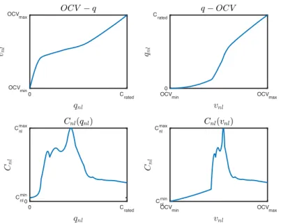
Figure 3-8: 𝐶𝑛𝑙(𝑞𝑛𝑙) and 𝐶𝑛𝑙(𝑣𝑛𝑙) of a typical 𝑂𝐶𝑉 − 𝑞 curve. ... 40

Figure 3-9: TM modified with an affine capacitor. ... 41

Figure 3-10: The TM with the self-discharge resistance in parallel to the affine bulk capacitor. ... 42

Figure 3-11: The setup of an EIS experiment. ... 43

Figure 3-12: Typical Nyquist plot of the internal impedance of a Li-ion battery. ... 44

Figure 3-13: The general EIS model of the internal impedance of a battery. ... 44

Figure 3-14: The approximated RI. ... 45

Figure 3-15: 𝑆𝑜𝐶 and 𝑇 dependences of an AESC LMO battery. ... 47

Figure 3-16: Variations with 𝑇 and 𝑆𝑜𝐶, of the 𝑅𝑠 of an AESC LMO battery. ... 47

(12)

Figure 4-2: The TM with a nonlinear bulk capacitor. ... 48

Figure 4-3: Re-proposition of Figure 3-6. ... 50

Figure 4-4: The proposed model without the switching logic. ... 54

Figure 4-5: Re-proposition of Figure 4-1. The switching logic is in red. ... 55

Figure 4-6: Cell-model loaded by a current generator. ... 58

Figure 4-7: Cell-model loaded by a voltage generator. ... 59

Figure 4-8: Cell-model loaded by a resistor. ... 60

Figure 4-9: Circuital symbol of a diode showing the reference directions of 𝑣𝐷 and 𝑖𝐷. ... 61

Figure 4-10: 1𝑆1𝑃|𝑖. ... 66

Figure 4-11: 1𝑆1𝑃|𝑣. ... 67

Figure 4-12: 1𝑆1𝑃|ℛ. ... 68

Figure 4-13: Cell-model loaded by an EM. ... 69

Figure 5-1: Blue ZhiDou D1 model. ... 73

Figure 5-2: The CAN logger we used to extract the data from the car. ... 73

Figure 5-3: Data that clearly highlights the relaxation of the battery. ... 74

Figure 5-4: Data that explores the upper nonlinear region 𝑆𝑜𝐶 ∈ 96%, 100% of the 𝑂𝐶𝑉 − 𝑆𝑜𝐶 graph. ... 74

Figure 5-5: The 𝑂𝐶𝑉 − 𝑆𝑜𝐶 curve. ... 75

Figure 5-6: A rough estimate of the aggregate decay of the 'long ride' voltage profile. ... 76

Figure 5-7: Setup of the parameter estimation. ... 78

Figure 5-8: Calculation of the residuals. ... 79

Figure 5-9: Estimation results on ‘long ride’ data. 𝑆𝑜𝐶 ∈ 60%, 100%, 𝑇 ∈ 21˚C, 28˚C. ... 80

Figure 5-10: Residuals of Figure 5-9 ... 80

Figure 5-11: Estimation results on ‘run and pause’ data. 𝑆𝑜𝐶 ∈ 45%, 60%, 𝑇 ∈ 13˚C, 17˚C. ... 81

Figure 5-12: Residuals of Figure 5-11. ... 81

Figure 5-13: 𝑆𝑜𝐶 ∈ [60%, 76%], 𝑇 ∈ [13˚C, 17˚C]. ... 83

Figure 5-15: 𝑆𝑜𝐶 ∈ [57%, 72%], 𝑇 ∈ [11˚C, 14˚C]. ... 84

Figure 5-17: 𝑆𝑜𝐶 ∈ [39%, 55%], 𝑇 ∈ [10˚C, 14˚C]. ... 85

Figure 5-19: 𝑆𝑜𝐶 ∈ [33%, 44%], 𝑇 ∈ [11˚C, 14˚C]. ... 86

Figure 6-1: 1𝑆2𝑃. ... 89

Figure 6-2: How Δ𝑣, 𝑉, Δ𝑞 varies with 𝐶2𝑟𝑎𝑡𝑒𝑑. ... 96

(13)

Figure 6-4: 1𝑆2𝑃|𝑖. ... 98

Figure 6-5: a) 𝑢, b) 𝑖1 and 𝑖2, c) 𝑆𝑜𝐶1 and 𝑆𝑜𝐶2. ... 106

Figure 6-6: The states of cell 2’s switches and diodes. ... 106

Figure 6-7: 1𝑆2𝑃|𝑅. ... 107

Figure 6-8: 1𝑆2𝑃|EM. ... 112

Figure B-1: Nyquist plots of CPEs. ... 121

(14)

LIST OF ABBREVIATIONS

!NF: not normal form 51

BEMF: Back electromotive force 69 BMS: Battery management system i CPE: Constant phase element 121 ECM: Electrical circuit model i EIS: Electrochemical impedance spectroscopy 35 EKF: Extended Kalman filter 32

EM: Electric motor 14

EMF: Electromotive force 17

EV: Electric vehicle i

FEV: Fully electric vehicle 20 HEV: Hybrid electric vehicle 19 ICE: Internal combustion engine 14 ICV: Internal combustion vehicle i KCL: Kirchhoff's current law 50

KF: Kalman filter 32

KVL: Kirchhoff's voltage law 50

LCO: Lithium cobal oxide 27

LFP: Lithium iron phosphate 27

Li: Lithium 15

LMO: Lithium manganese oxide 27

LUT: Lookup table 49

makima: Modified Akima 49

MPE: Mean proportional error 82

NF: Normal form 51

NMC: Nickel manganese cobalt 27 𝑂𝐶𝑉: Open circuit voltage 23 ODE: Ordinary differential equation 50 PEV: Plug-in electric vehicle 20 PHEV: Plug-in hybrid electric vehicle 20

PS: Parallel of series 19

RI: Randles impedance 43

SEI: Solid electrolyte interface 20

𝑆𝑜𝐶: State of charge 16

𝑆𝑜𝐻: State of health 25

SP: Series of parallels 19

𝑇: Battery temperature 22

TEC: Thévenin equivalent circuit 17

TI: Thévenin impedance 45

(15)

1. INTRODUCTION

1.1 The bigger picture

Global warming is propelling the sixth mass extinction of life on earth: including that of human civilization. In response, the great majority of countries have ratified the Paris agreement, which sets out the collective goal of “holding the increase in the global average temperature to well below 2˚C above pre-industrial levels and pursuing efforts to limit the temperature increase to 1.5˚C [...]; recognizing that this would significantly reduce the risks and impacts of climate change” [1]. Hitting this target requires a considerable reduction of the global emissions of greenhouse gases expelled by human activities.

By popularizing full EVs and enabling power plants to store the excess energy they generate1_{, the much}

sought after breakthrough in the performance of batteries would cover a significant share of this reduction. The transportation and power sectors account for 40% of all greenhouse gas emissions, and the battery value-chain must grow 19 times its current size to cover 30% of the CO! reduction required in these industries by 2030 [2]. This corresponds to 12% of the required global reduction.

This paper focuses on ‘EVs’, which are vehicles with an electric motor (EM). They are in contrast to ICVs, that rely exclusively on an internal combustion engine (ICE). Some EVs also have an ICE, so ‘full EVs’ is the term used to classify vehicles that have only an EM. EVs power their EM by a battery, while ICEs are powered by fuel tanks. The battery of EVs are composed of many electrochemical cells because modern cell technology is not able to meet the requirements of EV applications with just one cell.

Electrochemical cells are split into three categories: galvanic, electrolytic, and rechargeable. A galvanic cell is an energy converter that stores chemical energy and transforms it into electrical energy2_{[3]. The electrolytic}

cell is the device that performs the reverse conversion, and the rechargeable cell does both. EV batteries are made up only of rechargeable cells, so we refer to them simply as ‘cells’ from now on.

Even though an EV’s purchase price is generally higher than that of an ICV, EVs can save up money in the long term because grid energy is much cheaper than petroleum fuel and because EMs are much more efficient than ICEs3_{. On this last note, EVs are very often presented as an eco-friendly alternative to ICVs, but they are}

1_{This would be especially useful for plants running on renewable sources, as their profile of daily power generation is}

highly skewed with respect to that of daily power demand [49].

2_{It’s an invention that changed the world by enabling the mobile use of electrically-powered devices [4].} 3_{75% efficiency for EMs compared to just 20% for ICEs [50].}

(16)

currently not nearly as clean as they are made out to be. Even though EVs may not pollute locally, the plant that charged them polluted elsewhere — i.e. unless it ran on renewables. Until all grids are powered by renewables any claim that full EVs operate carbon-neutrally will be false.

The current technology powering EVs and all new electrical devices, is the mature but still promising lithium-ion (Li-lithium-ion) technology. Sustaining the aforementlithium-ioned expanslithium-ion in the productlithium-ion of Li-lithium-ion batteries will require a significant increase in energy and mining, defeating the objective of eco-friendliness. That is, unless that energy is delivered by renewables and the recycling of batteries is boosted. Recycling must be enhanced because the extraction of essential materials such a lithium and cobalt have considerable ecological and social impacts seldom acknowledged by scientific papers.

An EV battery contains 10kg − 15kg of lithium [5], and their popularization is expected to grow the throughput of lithium mining exponentially [6]. This will intensify the pumping of the underground brine that contains the lithium, further straining the water supplies on which local communities depend on. It will also worsen droughts in the areas surrounding the lithium mines, as about 2kL are needed to extract 1 tonne of lithium [6]. Extraction and pollution can be mitigated by recycling the lithium in existing batteries. On a side note, even though transitioning from petroleum is believed to have the potential of eradicating war and foreign meddling in the middle east, it already seems that the instability would only be moved to lithium-rich places like the 'lithium triangle' of South America [7]. In fact, former Bolivian president Evo Morales accused foreign powers to have meddled in favour of his ousting because of the country wanted to nationalize its lithium industry [8].

Cobalt mining has a severe human cost, as well as having a considerable environmental footprint. Two thirds of all cobalt is mined in the Democratic Republic of Congo [2]. The miners — a lot of whom are children — work in hazardous conditions, oftentimes without protective gear. The prolonged exposure to cobalt causes, birth defects, contact dermatitis and hard metal lung disease: a potentially fatal respiratory illness [2], [9]. By 2030, every EV battery will contain 8kg of cobalt, so advances in recycling would help lower the demand of new cobalt provided by an exploitative industry [2]. This is yet another example of how a circular economy can achieve both social and ecological sustainability.

With an increasing population and the deepening of urbanization, ownership of automobiles is growing and with it, traffic congestion and environmental pollution. Along with the principles of a circular economy, a sharing business model also prevents the over-production of batteries, but by improving the utilization rate of cars. In doing so, car-sharing also manages to reduce exhaust pollution, fuel emissions and the social public space dedicated to cars. Additionally, it has the potential to save the user about 70% of the cost of travel, comprised of things such as fuel costs, maintenance fees and parking fees [10]. The car on which we ran our

(17)

tests is in fact part of the fleet of an Italian car-sharing firm, Share N’ Go. The EV industry is one of the first to seriously practice the principles of a sharing economy. It could accustom the public to a sharing lifestyle that extends beyond the automobile sector, and that has the potential of optimizing the use of social resources.

It is also worth noting that we are at the cusp of the fourth industrial revolution, which will connect all electrical devices and enable the replacement of human-driven cars by self-driving cars. The battery industry must find itself ready to power this new generation of cars so that all internal combustion cars are naturally removed from circulation.

Along with the recycling and improvement of batteries, also their safe, efficient, and long-lasting use will help power sustainable and just economic growth. By focusing on their modelling, this is the aspect of batteries that the paper contributes to. In fact, an EV’s battery is managed by the BMS, which references a model of the battery to estimate some important quantities, such as its remaining charge. However, the model stored within the BMS accounts only for quantities at battery-pack level, and not those at the level of the individual cells. It is actually just a scaled-up version of a cell-model, which acts as a very good approximation when the cells operate in similar conditions and very similar themselves.

1.2 Raison d’être of the work

If the model of the battery-pack must account for things such as mismatches between the cells, or distributed phenomena like thermal gradients4_{, then each cell must be represented individually in a multi-cell model.}

Our application is to study how mismatches between the cells of a battery-pack affect their rates of discharge. It is thus an offline application, with no constraint on time or complexity. The mismatches could be faults, or statistical variations that arose from manufacturing. The study of mismatches can give insight into how the cells should be placed, or how the packaging of the battery should be designed to mitigate the effects of the mismatches.

That being said, we were not able to conduct our study on mismatches because there was not an electrical cell-model with which a coherent multi-cell model could be built. Thus, we had to focus on designing one instead. Nevertheless, we will also provide the tools and formalisms for others to pursue our initial objective. The cell-model will be built with our application in mind, so it will only represent phenomena that have to do with the state of charge (𝑆𝑜𝐶) of the cell.

(18)

The pre-existing ECMs were inadequate because they cannot model a cell’s behaviour when its completely (dis)charged. The reason being that all ECMs are built for online applications, where the BMS prevents the cells from charging or discharging completely, so they need not account for this behaviour. However, ours is an offline application, meaning that a BMS does not come to our rescue.

1.3 Synopsis

There is a trade-off between the accuracy of a model and its computational efficiency; by consequence, the field of battery modelling splits into two categories: chemical and electrical modelling. The former builds the model on chemical and thermodynamic first-principles, while the latter builds a 1-port electrical circuit that mimics the I/O behaviour of the battery. Chemical modelling is more accurate, but it is much heavier computationally, and it is only implementable offline unless major simplifications are made. On the other hand, ECMs abstract away the internal physics of the battery, enabling single-cell ECMs to always be implementable online by the BMS.

However, when transitioning from a single-cell model to a multi-cell model, the computational complexity increases with each new cell. Our cell-model must therefore be as light as allowable by the phenomena we want to represent. An ECM will thus suffice, so we will focus primarily on electrical circuit modelling; covered in chapter 3.

The electrical power that a battery injects into the circuitry originates from the internal reactions transducing the chemical energy stored within it. If it's only the injection of electrical energy that needs to be considered, a voltage generator representing the electromotive force (EMF) of the battery suffices. However, it is experimentally observed that the steady-state voltage across the battery's terminals depends on the load, meaning that the battery’s internal resistance must be represented in series to the EMF generator. The resulting circuit is the Thévenin equivalent circuit (TEC) of the battery. Furthermore, batteries also display exponential relaxation dynamics, which can be modelled adding 𝑅𝐶-parallels in series to the TEC. With the addition of dynamical elements, the equivalent resistance becomes an equivalent impedance. All ECMs of batteries are impedential TECs, with their equivalent impedance used to account for the nonidealities of the battery with respect to the ideal voltage generator.

Since the charge is directly related to the chemical energy stored by the battery, its conversion to electrical energy can be accounted for, from a circuit theory perspective, using a bulk capacitor in place of the voltage generator. By acting as a reservoir of charge (much like a battery does), the charge on the bulk capacitor represents the charge stored by the battery. It is experimentally observed that the equivalent capacitance of a battery varies with the charge it stores, indicating the need of a nonlinear bulk capacitor. That being said,

(19)

most of the time this behaviour is neglected, and a linear bulk capacitor is opted for instead. However, our application needs to represent the steady-state behaviour as accurately as possible, so our model will adopt a nonlinear bulk capacitor. The model will be built in chapter 4, and in chapter 5 we’ll use it to identify a LiMn_!O_" battery-pack. On this note, it will suit us to eventually centre all discussions around the LiMn!O" chemistry. For example, the cell-model will disregard phenomena that are neglectable in LiMn!O" cells, but not necessarily in cells of other chemistries. The system identification will demonstrate the proper functioning of the model’s constituent nonlinear capacitor, which we had to code ourselves due to its absence in Simscape’s library.

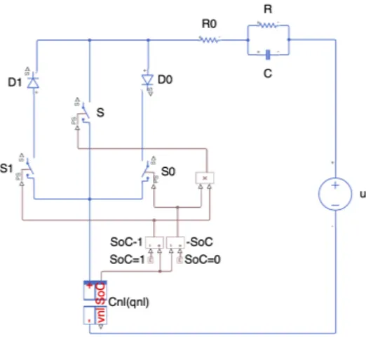
The nonlinear capacitor will be governed by the battery’s voltage-charge relation at zero-current steady-state, i.e. its 𝑂𝐶𝑉 − Q curve. Seeing as a Li-ion battery can contain only so much lithium, its 𝑂𝐶𝑉 − Q curve is defined only on a finite interval of charge. This is a problem because simulators cannot work with bounded state-variables, but can only work in a state-space that corresponds to ℝ#_{. To address the issue, this work} innovates a simple switching system that prevents the charge from overflowing from its region of definition during simulation. In so doing, the switching system makes the cell-model coherent for multi-cell modelling, allowing for a complete representation of inter-cell interactions.

With the proposed model now at our disposal, chapter 6 formalizes the study of mismatches. We will focus primarily on the simple, but exhaustive case of two cells in parallel. The state of this system will be transformed to put in evidence the mismatches between the corresponding state-variables of the two cells. We will only hint on how to extend all the reasonings to more cells.

The results of the thesis are presented in chapters 4, 5, and 6, at the end of which they are evaluated. These ‘chapter evaluations’ propose ways in which to improve the work conducted in their chapters, and ways in which to build upon it. The reader should consider them as part of chapter 7. CONCLUSION, which only summarizes the thesis.

Chapter II will now introduce battery packs, review the working principles of cells, introduce typical quantities of batteries and their orders of magnitude, and review the major techniques for the estimation of the energy remaining within a battery.

(20)

2. THE BASICS OF Li-ION BATTERIES

2.1 Battery-packs (sSpP) and electric vehicles (EVs)

To meet the car’s energetic demands, its battery is comprised of many smaller batteries. This text will use the following definitions:

Cell: the fundamental bilateral electrochemical energy converter. String: a package of cells connected in series.

Module: a package of cells connected in parallel.

Battery-pack: a package of either, strings connected in parallel or modules connected in series. Refer to Figure 2-1.

We will adopt the convenient notation used by [11], where sSpP (Series of Parallels) denotes a battery-pack comprised of s modules in series, each made up of p cells in parallel, and pPsS (Parallel of Series) denotes one comprised of p strings in parallel, each s cells long. So sS1P and 1PsS refer to a string of s cells while 1SpP and pP1S refers to a module of p cells. Seeing as Li-ion cells are very intolerant to overcharging and over discharging, Li-ion battery-packs are only ever configured as series of parallels [12]. Thereby, we will speak only of this configuration.

Given that EMs are powered by battery-packs and ICEs by fuel tanks, the following terms make up the taxonomy of EVs:

Electric vehicle (EV): a vehicle with an EM for propulsion.

Hybrid electric vehicle (HEV): an EV that also has an ICE for propulsion. The battery charges from recovered kinetic energy of the car, e.g. through regenerative braking [11]. The two different

(21)

motors are more efficient in different phases of a drive cycle, so by switching between the two accordingly, the HEV is able to be more efficient in its power consumption [11].

Plug-in hybrid electric vehicle (PHEV): a HEV whose battery can be charged when hooked to an external source of power, like an electric grid [11]. The PHEV is propelled only by its EM until the battery runs out, after which the PHEV acts as a regular HEV. A PHEV prioritizes its EM.

Fully electric vehicle (FEV): an EV that has only an EM for propulsion.

Plug-in electric vehicle (PEV): a FEV whose battery is charged by hooking it to an external source of power, like an electric grid [11].

Cells are connected in series to increase the voltage of the battery-pack, while they are connected in parallel to increase its capacity [11]. Battery-packs for automotive applications need to be able to deliver hundreds of kilowatts, that requires strings of lengths in the order of tens of cells, which correspond to voltages of around 80V [11]. The battery-pack of an HEV is usually just a string of cells, while PHEVs and PEVs require cells to be placed in parallel to meet their greater requirements on autonomy [11]. “It is more economically [and technologically] feasible (and thermally desirable) to use multiple cells in parallel [to make up a module] rather than a single, large-capacity cell.” [11].

2.2 Internal workings of a lithium-ion (Li-ion) battery cell

Referring to Figure 2-2, a cell is composed of four basic elements: an electrolyte, a separator, and two electrodes (one denoted as positive and the other as negative). Li-ion cells also form a passivation layer between the negative electrode and the electrolyte, called the ‘solid electrolyte interface’ (SEI).

The negative electrode is the one at lower electrical potential [13], from which electrons leave the battery when it is supplying power. It is usually composed of graphite 𝐶$, an electrically conductive solid allotrope of carbon, made up of layered and loosely held sheets of tightly bonded carbon atoms [14].

(22)

The positive electrode is the one at higher electrical potential [13], from which electrons enter the battery when it is supplying power. The positive electrode is usually made up of a metal oxide, such as cobalt oxide (CoO!), manganese oxide (Mn!O"), iron phosphate (FePO"), nickel manganese cobalt oxide (NiMnCoO!), or others [13].

The ‘anode’ is the electrode that undergoes oxidation (loss of electrons) while the ‘cathode’ is the electrode that undergoes reduction (gain of electrons) [14]. During discharge, the negative electrode of the battery is the anode and the positive electrode is the cathode. Otherwise, during charging, the positive electrode is the anode and the negative electrode is the cathode.

The lithium radical is very reactive, so it must be handled carefully [15] and is why Li-ion batteries rely on the principle of ‘dual-intercalation’ [16]. ‘Intercalation’ is the insertion of a guest species into a host lattice [17], while ‘dual-intercalation’ is a term denoting that the lithium ion — the guest species —can be soaked up by both electrodes. Specifically, the lithium atoms housed in the anode lose their electrons to the external circuit and de-intercalate from the anode towards the cathode (through the electrolyte), into which they then intercalate and reduce with the electrons from the external circuit. In the graphite electrode, the lithium radicals are housed between its molecular sheets, while the positive electrode houses them inside its metal oxide lattice.

The ‘chemistry’ of a Li-ion battery is the material used for the positive electrode (e.g. Mn!O"), prefixed by lithium (e.g. LiMn!O"). That is, the composition of the positive electrode when the battery is completely discharged and all the lithium is housed in the positive electrode.

If the more performant lithium metal were used as the negative electrode, during charging the lithium ions would deposit onto it as lithium atoms. However, this allows for lithium dendrites to grow from the negative electrode to the positive electrode: short-circuiting them. The use of graphite prevents dendrites from growing because the lithium is housed rather than deposited [13], [18].

In the case of the LiMn!O" chemistry, the processes of intercalation, de-intercalation, reduction and oxidation are described in the following chemical formulas:

Discharging: b−: LiC$ %&. cd Li(_{+ e})_{+ C} $ +: Li(_{+ e})_{+ Mn} !O_{" *+,.}c⎯d LiMn!O" LiC_$+ Mn_!O_"⟶ LiMn_!O_"+ C_$ (2.1)

From the total equation, we see that during discharging, the lithium de-intercalates from the sheets of the graphite 𝐶$ and intercalates into the Mn!O" lattice.

(23)

Charging: b+: Li(+ e)+ Mn!O" %&. hi LiMn!O" −: LiC_{$ *+,.}h⎯i Li(_{+ e})_{+ C} $ LiC$+ Mn!O"⟵ LiMn!O"+ C$ (2.2)

From the total equation, we see that during charging, the lithium de-intercalates from the Mn!O" lattice and intercalates between the sheets of the graphite.

LiC_$+ Mn_!O_"

-./01234.54 c⎯⎯⎯⎯⎯⎯⎯d 61234.54

h⎯⎯⎯⎯⎯i LiMn!O"+ C$ (2.3) The electrolyte is a material or substance that is ionically conducting, but not electronically [14]. That is, it is porous only to the lithium ions and not to the electrons they lost [15]. This forces the electrons to go through the external circuit to re-bond with the lithium ions at the cathode. It is thanks to the electrolyte that a battery can power an external load. It’s important to note that: while electrolytes conduct current composed of ions, the electrodes conduct current composed of electrons [14]. The electrolyte obviously poses resistance to the ionic current that passes through it, contributing to the internal resistance of the cell [19]. Lithium is highly reactive with water, so organic liquid electrolytes are opted over aqueous electrolytes. “The electrolyte used varies based on the choice of electrode materials[.] […] Li-ion battery electrolytes [for EVs] are usually based on an organic solvent loaded with a lithium salt. A common system is the use of an organic carbonate, such as Ethyl carbonate, propylene carbonate, [or] dimethyl carbonate, with dissolved LiPF$, LiBF_" or LiClO".” [20].

The separator is a barrier immersed within the electrolyte and permeable to the traversing ions. It is a safety measure against any possible contact between the electrodes, and against flammability [20]. In fact, the temperature of the cell (𝑇) diverges if it reaches that of the thermal runaway, causing the battery to catch fire. The separator protects the battery by shutting it down before it can ever reach the thermal runaway [21].

The SEI is permeable to the lithium ions, but not to the electrons [22], and it forms on the negative electrode as the lithium graphite reacts with the organic electrolyte during the first charging [13]. This reaction yields the products that compose the SEI, like Li!O, LiF, LiCl, Li!CO7, alkoxides and nonconducting polymers [23]. Once formed, the SEI remains, making the lithium that it is composed of irretrievable to transfer charge. This results in a loss in the cell’s capacity. That being said, the battery would not work without the SEI, as it acts as a passivation layer that inhibits any further reaction between the electrode and the electrolyte. That is, it prevents the battery from eating itself. “The SEI […] could be broken up and it is subject to degradation due to both current and temperature cycling. Consequently, the SEI is re-formed each time the electrode’s surface is directly exposed to the electrolyte” [13]. This means that lithium that was once available to transfer

(24)

charge is lost to repairing the SEI; contributing to the capacity-fade that the cell experiences throughout its lifetime.

2.3 Definition of the open circuit voltage (𝑂𝐶𝑉) and of the state of charge (𝑆𝑜𝐶)

All the terms introduced in this section may refer to a cell, string, module, or an entire battery-pack. Therefore, to make things simpler, this text will use ‘battery’ as the indiscriminate denomination.

Battery: a cell, module, string, or battery-pack.

The following two quantities are independent of things such as temperature and pressure [24].

Capacity of the battery (C): the amount of lithium within the battery that is effectively available to transfer its ionic charge [25]. This amount is measured in units of charge because each concerned lithium atom corresponds to an ion with charge 𝑒.

Charge of the battery (Q): the amount of lithium (in units of charge) within the negative electrode and effectively available to transfer its ionic charge [25].

Q ∈ [0, C], but the BMS restricts the battery’s operation within a subinterval [Q89#, Q8:;] because working all along [0, C] degrades the battery too quickly for automotive applications [25]. The subinterval is chosen in such a way that the battery meets the lifetime and voltage requirements of the application it is intended for. Hence, the lifetime specification provided by the manufacturer corresponds to an operation of the battery that is restricted to [Q89#, Q8:;]. All this leads us to define the following quantities:

Deliverable charge (Q<=>9?=@:A>=): the charge that falls within the subinterval [Q89#, Q8:;]. Deliverable capacity (𝐶<=>9?=@:A>=): the width Q8:;− Q89# of the subinterval [Q89#, Q8:;].

The only way in which Q can be measured is by depleting the battery of all its charge, and then returning it if the observer effect needs bypassing, as it would need to be in automotive applications. However, this method is too disruptive and too time consuming for automotive applications, so Q must be estimated. Enter the 𝑂𝐶𝑉 − Q relationship of the battery:

Open circuit voltage (𝑂𝐶𝑉): the steady-state5_{voltage across the battery when it is not connected}

to anything. The 𝑂𝐶𝑉 of the battery corresponds to its EMF [26].

(25)

Given a properly designed battery, the relationship between its 𝑂𝐶𝑉 and its Q will be strictly increasing. Therefore, it will be invertible, and Q will be derivable from the 𝑂𝐶𝑉 of the battery. The measurement of Q is thus brought back to the measurement of the 𝑂𝐶𝑉, which is not at all intrusive. We will denote this as the 'voltage method', and we will treat it in greater detail in section 2.6.1.1. The 𝑂𝐶𝑉 − Q relationship varies with the chemical equilibrium [27] and the usage 𝓊 of the battery. In automotive applications, only temperature variations will noticeably impact the chemical equilibrium of batteries, so 𝑂𝐶𝑉(Q, 𝑇, 𝓊), and we define 𝑂𝐶𝑉89#( 𝑇, 𝓊) ≜ 𝑂𝐶𝑉(Q89#, 𝑇, 𝓊) and 𝑂𝐶𝑉8:;( 𝑇, 𝓊) ≜ 𝑂𝐶𝑉(Q8:;, 𝑇, 𝓊) . Unless the dependence of the 𝑂𝐶𝑉 − Q curve on ( 𝑇, 𝓊) is accounted for, the voltage method can only act as an estimate of the charge.

Seeing as automotive applications deal only with the deliverable charge, the EV battery community is accustomed to working in the following reference system:

𝑞 ≜ Q_<=>9?=@:A>=− Q_89# 𝑞 ∈ [0, 𝐶_<=>9?=@:A>=]

From now on with "charge of the battery" we will mean 𝑞, and with "capacity of the battery" we will mean 𝐶_<=>9?=@:A>=; aligning our terminology to that used in the literature of EV batteries. The quotient of these quantities defines the ‘state of charge’ 𝑆𝑜𝐶 of the battery [25]

𝑆𝑜𝐶 ≜ B

C!"#$%"&'(#" (2.4) which is a unitless expression of the deliverable charge. 𝑆𝑜𝐶 = 0 is the state of the battery at which it is considered to be empty, and 𝑆𝑜𝐶 = 1 is the state at which it is considered to be full. Needless to say, 0 ≤ 𝑆𝑜𝐶 ≤ 1.

In the literature, there is not a regimented distinction between 𝐶<=>9?=@:A>= and the

Discharge capacity (𝐶<9DEF:@G=): the charge removed from the battery as it is discharged at a constant rate from 𝑆𝑜𝐶 = 1 up until the battery voltage 𝑣 reaches 𝑂𝐶𝑉89#( 𝑇, 𝓊) [25].

because both are referred to as the capacity of the battery by different texts, but they are different. Seeing as the definition of 𝐶<9DEF:@G= refers to 𝑣 and not 𝑂𝐶𝑉, 𝐶<9DEF:@G= depends on the internal resistance of the battery, its current and its temperature (see section 2.5.1) [25]. Also, the battery will not have discharged completely because 𝑣 = 𝑂𝐶𝑉89# does not correspond to 𝑆𝑜𝐶 = 0 [25], so 𝐶<9DEF:@G= ≠ 𝐶<=>9?=@:A>=. Having defined 𝐶<9DEF:@G= we can now define the

Rated capacity ( 𝐶@:H=<): the average discharge capacity, measured at a specified load and temperature, of a test group of brand-new batteries (𝓊 = 0) [25].

(26)

which is what manufacturers provide as the capacity of their battery. This is because the capacity of a battery is too cumbersome to measure, let alone for every battery that is produced. We will call ‘rated conditions’ the conditions at which 𝐶@:H=< is defined. With this said, 𝐶<9DEF:@G=q_@:H=< does not correspond to 𝐶@:H=< because 𝐶@:H=< is not specific to the battery in question, but it is the average value of many cells of the same design. It’s common to use 25˚C as the rated temperature and a 1C discharge current as the rated load [25]. 1C is the constant current required to completely discharge the battery in one hour, starting from its full state [28].

Seeing as both 𝑞 and 𝐶<=>9?=@:A>= are not easily measurable, all we can hope for is an estimate 𝑆𝑜𝐶r of the

𝑆𝑜𝐶 .

𝑆𝑜𝐶r ≜ BI

C&')"! (2.5)

𝑞 can be estimated via many different techniques (some of which are treated in section 2.6.1 [28] while 𝐶_@:H=< can act as an estimate of 𝐶<=>9?=@:A>= when 𝐶<=>9?=@:A>= isn’t measured by the user, as is our case. At the end of this section, we will forget of definition 2.4 and instead use

𝑆𝑜𝐶 ≜ B

C&')"! (2.6)

as definition of the 𝑆𝑜𝐶 because that is the one adopted by the literature. Either way, 𝑆𝑜𝐶r is an estimate of 𝑆𝑜𝐶.

The estimation of the 𝑆𝑜𝐶 is said to be ‘online’ when it is running alongside the operation of the battery, and it is said to be ‘offline’ when it is made only once the battery has stopped being in operation. In the first case, the estimation is made on real-time data, while in the second case it is made only after the observation period has expired and all the data has been collected.

As already mentioned, a battery progressively loses lithium to irreversible processes6_{occurring within it.}

Therefore, 𝐶<=>9?=@:A>= decreases as the battery is used, meaning it can be employed to track the battery’s aging. 𝐶<=>9?=@:A>=(𝓊) ≤ 𝐶<=>9?=@:A>=(0) at any point in the battery’s life cycle, so the ‘state of health’ (𝑆𝑜𝐻)

𝑆𝑜𝐻(𝓊) ≜C!"#$%"&'(#"(𝓊)

C!"#$%"&'(#"(M) (2.7) acts as a measure of the battery’s aging [29]. Needless to say, 0 ≤ 𝑆𝑜𝐻 ≤ 1.

𝑆𝑜𝐻 cannot be measured online because 𝐶<=>9?=@:A>=(𝓊) can only be measured offline. Having said this, it does not need to be measured online because the aging process of a battery is much slower than a typical

(27)

charge-discharge cycle, meaning that the most recent offline estimate of the 𝑆𝑜𝐻 will be valid for any online calculations. In theory, this measurement could be carried out by the BMS any time the vehicle recharges from its ‘empty’ state to its ‘full’ state [30]. However, in the end it will only able to yield an estimate of the present 𝐶<=>9?=@:A>=. 𝐶<=>9?=@:A>=(0) is unknown, but could be estimated with 𝐶@:H=< [28] to give

𝑆𝑜𝐻r (𝓊) ≜CN!"#$%"&'(#"(𝓊)

C&')"! (2.8)

which can yield a better estimate 𝑆𝑜s𝐶 of the 𝑆𝑜𝐶 𝑆𝑜s𝐶 ≜OPCQ OPR S = * + ,&')"! , -!"#$%"&'(#" ,&')"! = BI CN!"#$%"&'(#" (2.9) In the end however, our application does not deal in characteristic times where aging processes become apparent, so the 𝑆𝑜𝐻 won’t be appearing anywhere in this work.

2.4 State of the art of the Li-ion technology

Figure 2-3 shows there is a trade-off between the power density and the energy density of cells, and that the advancement of cells technology seeks to enhance both these quantities. In this quest, cells have transitioned from being Pb-based, to being Ni-based to now being Li-based [20]:

Energy density: the storable energy per unit volume [3].

Power density: the maximum deliverable power per unit volume [3]. Specific energy: the storable energy per unit mass [3].

Specific power: the maximum deliverable power per unit mass [3].

Figure 2-3: A log-lin comparison of the energy and power requirements of different types of EVs, versus the energy and power performances of different cell technologies. Reprinted from [31].

(28)

Figure 2-3 also shows that only a few cell technologies have the potential to meet both energy and power density requirements for HEVs, PHEVs or PEVs [31]. Table I in appendix A presents various cell requirements for different types of EVs, while Table II summarizes the characteristics of various cell chemistries. Particular interest should be dedicated to the manganese spinel LiMn!O" entries because it is the chemistry of our test battery. This is an outdated EV battery as “pure Li-manganese batteries are no longer common today. Most Li-manganese batteries blend with NMC to improve the specific energy and prolong the life span.” [20]. LiCoO! (LCO) was the first commercially mature lithium-cell chemistry. It has a high energy density, but suffers from a short cycle life and thermal instability. This last shortcoming requires restricting the current to keep the temperature below that of LCO’s thermal runaway, which is rather low. By sacrificing energy density with respect to LCO, LiMn!O" (LMO) has a longer lifespan and is also more thermally stable thanks to its lower internal resistance, which allows for greater currents. With respect to LMO, LiFePO" (LFP) improves slightly on all the aforementioned aspects, but at the cost of worse self-discharge, lower voltage, and considerable degradation when exposed to moisture. Also LiNi&MnTCoU)&)TO! (NMC) is able to improve on every aspect of LMO, but only slightly sacrificing thermal stability: making it the most performant chemistry [20]. Even though LCO is seldomly used anymore, none of these alternative chemistries can match its energy density. What has been said in this paragraph is summarized succinctly in the spider charts of Figure 2-4 and in more detail in Table II.

Figure 2-4: Spider charts that compare various chemistries against a plethora of criteria. Reprinted from [20]. For each metric, the outer hexagon is the most desirable.

(29)

2.5 𝑂𝐶𝑉 − 𝑆𝑜𝐶 curve of a battery

Depending on the chemistry and the manufacturing process of the Li-ion cell, its 𝑂𝐶𝑉 − 𝑆𝑜𝐶 characteristic usually either looks like Figure 2-5, Figure 2-6 or Figure 2-7: all of which are strictly increasing. While both Figure 2-5 and Figure 2-6 have a central “linear” (it’s actually affine) region, Figure 2-7 has two that are connected by a transition region. The central linear region of Figure 2-5 sees a nonlinear region to its right while that of Figure 2-6 sees a linear one. The linear region usually spans the great majority of the 𝑆𝑜𝐶-interval, so for convenience the BMS of many cars restrict the battery from operating outside it.

Figure 2-7: The constant current (𝑖 ≠ 0) discharge profile of a charged LMO cell. Adapted from [56]. It has the same shape as the cell’s flipped 𝑂𝐶𝑉 − 𝑆𝑜𝐶 curve because the ordinate is the constant current (𝑖 ≠ 0) steady-state voltage of the battery, and the abscissa is the charge extracted. The profile shows that the 𝑂𝐶𝑉 − 𝑆𝑜𝐶 curve has two separate linear regions connected by a central transition region. It’s thus very likely that our LMO battery-pack has more than one linear region.

Figure 2-6: 𝑂𝐶𝑉 − 𝑆𝑜𝐶 characteristic of an LCO cell [28]. Adapted from [58].

Figure 2-5: 𝑂𝐶𝑉 − 𝑆𝑜𝐶 curve of a 18650 LFP cell. Reprinted from [57]. The central linear region is surrounded by nonlinear ones.

(30)

2.5.1 Temperature (𝑇) dependence of the 𝑂𝐶𝑉 − 𝑆𝑜𝐶 curve

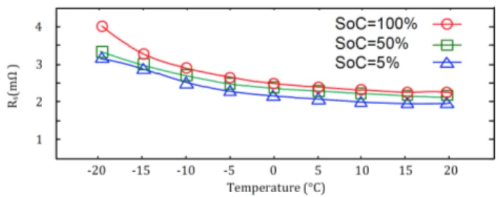
Figure 2-8 shows how 𝑇 affects the 1C discharge voltage profiles. The profiles are 𝑂𝐶𝑉|BWC_V &')"!)U6⋅H_lowered by the voltage drop across the internal resistance of the battery. The discharge profiles lower as 𝑇 decreases because the internal resistance increases (exponentially), as shown in Figure 2-9. What can be concluded from the discharge profiles is that 𝑂𝐶𝑉 − 𝑞 retains the same general waveform7_{, but with a linear region}

that steepens as the 𝑇 decreases. Nevertheless, accounting for 𝑇 is not necessary to build a cell-model that can act as the building block of a multi-cell model, so we will not account for it; even though the cell-model can be extended to do so.

2.6 Battery management system

With the goal of maximizing the longevity and the performance of the battery, the BMS is tasked with managing it as safely and reliably as possible [32]. The BMS bases the manipulation of the battery on measurements of its current and voltage, as well as on the voltages and temperatures of all the modules [33]. With these measurements, it is also able to estimate the 𝑆𝑜𝐶 and 𝑆𝑜𝐻 of the battery. BMS estimations of the 𝑆𝑜𝐶 are online and model-based, meaning that it should store a simple model of the battery that is fast enough on an inexpensive microprocessor unit [34]. The basic structure of a BMS is shown in Figure 2-10.

7_{In general, the 𝑂𝐶𝑉 − 𝑆𝑜𝐶 curve is able to retain its overall shape with variations of 𝑇, aging and current [51]. The}

curve depends on the sign of the current through a phenomenon known as ‘hysteresis’, which will be explored in section 3.2.1.1. However, any dependence on the magnitude of the current is tricky to study, but it is either negligible or non-existent.

Figure 2-8: Constant rate discharge voltage profiles of an LMO at different temperatures, with Li4Ti5O12 as its

negative electrode. Reprinted from [59].

Figure 2-9: Internal resistance of an LFP at varying temperatures and currents. Reprinted from [60].

(31)

Some of the things that the BMS does are:

· Prevent the over-charging and over-discharging of the cells, which cause internal damage [35]. The BMS cannot access to the individual cells directly, but only indirectly at module level.

· Rebalance the cells of the battery so their 𝑆𝑜𝐶𝑠 are as uniform as possible [33]. Cell rebalancing is crucial to talk about the not so well defined 𝑆𝑜𝐶 of a battery-pack [24].

· Diagnose battery faults [32]. Something that multi-cell models can help with.

2.6.1 Techniques of 𝑆𝑜𝐶 estimation

The 𝑆𝑜𝐶 is a pivotal quantity and must be estimated as accurately as possible. For example, the more accurate 𝑆𝑜𝐶r is, the less over-engineering is needed to mitigate issues like over-(dis)charging [36]. When we validate our model in chapter 5, we will have to estimate the 𝑆𝑜𝐶 from the voltage and current data collected by the BMS. Therefore, we include here the main ways by which the 𝑆𝑜𝐶 can be estimated.

(32)

2.6.1.1 Voltage method

As depicted in Figure 2-11, the voltage method uses the 𝑂𝐶𝑉 − 𝑆𝑜𝐶 curve to infer the 𝑆𝑜𝐶 from the measurement of the 𝑂𝐶𝑉. This will always be possible with properly designed batteries because their characteristic will be strictly increasing: i.e. invertible.

To use this method, the 𝑂𝐶𝑉 − 𝑆𝑜𝐶 characteristic of the battery must be known. The curve can be provided by the manufacturer or retrieved experimentally. Manufacturers seldomly provide the curve, so characterizing it oneself is usually the way to go. Reconstructing the curve entails interpolating an LUT of numerous (𝑆𝑜𝐶, 𝑂𝐶𝑉) datapoints collected at the same temperature. This procedure should then be repeated at many different values of temperature to construct a bidimensional lookup table (𝑆𝑜𝐶, 𝑇, 𝑂𝐶𝑉) [29], which is then be interpolated.

However, by definition, the 𝑂𝐶𝑉 can be measured only once the battery has relaxed, which requires the current/car to be null/off for some thousands of seconds. This means that the voltage method can only be used offline.

As a workaround, the voltage method is instead applied to an online estimate of the 𝑂𝐶𝑉. As shown in Figure 2-12, 𝑂𝐶𝑉w is derived by feeding the real time 𝑣\𝑖 data tracked by the BMS to an identified model of the battery [28], making it a model-based estimate.

The main issue of the voltage method is the flatness of the linear region of the 𝑂𝐶𝑉 − 𝑆𝑜𝐶 characteristic, because a small error in 𝑂𝐶𝑉w, or the curve itself, amplifies into a considerable error in 𝑆𝑜𝐶r [34].

Figure 2-12: The workflow for the voltage method applied on an estimate of 𝑂𝐶𝑉. Reprinted from [28]. Figure 2-11: The voltage method of 𝑆𝑜𝐶 estimation. Adapted from [28].

(33)

2.6.1.2 Coulomb-counting method

Seeing as the 𝑆𝑜𝐶 is an estimate of the releasable charge within the battery, the most intuitive way to estimate it is by integrating the current that flows through the battery

𝑆𝑜𝐶r (𝑡) = 𝑆𝑜𝐶r (𝑡_M) −∫ 9(Z)<Z ) ).

C&')"! (2.10)

The accuracy of this technique depends on the accuracy of the measurement of the outgoing current 𝑖(𝑡), as well as the accuracy of the initial 𝑆𝑜𝐶.

The Coulomb-counting method is very susceptible to any disturbance, systematic error, or drift noise(𝑓 ≪ U

H)H.) afflicting the current. This is because, through the integral action, they corrupt the estimation more and more as time passes [34] and is why the estimate of the 𝑆𝑜𝐶 must be periodically recalibrated [36]. Having said this, the Coulomb-counting method is never adopted by a BMS [25], [28].

𝑆𝑜𝐶(𝑡M) can be estimated by applying the voltage method just before the car is turned on, when the battery is completely relaxed. If 𝑆𝑜𝐶(𝑡M) is estimated like so, we will say that the Coulomb-counting method is ‘voltage-based’. In this case, 𝑆𝑜𝐶r (𝑡M) will be affected by the error amplification caused by the linear region of the 𝑂𝐶𝑉 − 𝑆𝑜𝐶 curve; meaning that 𝑆𝑜𝐶r (𝑡) will be affected by both the current noise and voltage noise. This is the method which we’ll use in chapter 5 because our model can implement it seamlessly; thanks to the nonlinear capacitor integrating the current, and whose voltage-charge relation is the 𝑂𝐶𝑉 − 𝐶@:H=<⋅ 𝑆𝑜𝐶 curve itself.

2.6.1.3 State-observer

The state of a system is the smallest set of its variables such that once they are known at a point 𝑡M in time, the output of the system for 𝑡 ≥ 𝑡M is independent of the values that the system’s inputs have taken up before 𝑡M. This means that these variables — the state-variables — have memory, and seeing as 𝑞(𝑡) = 𝑞(𝑡_M) + ∫ 𝑖(𝜏)𝑑𝜏_HH

. the charge of the battery is a state-variable of the battery and so is its 𝑆𝑜𝐶.

All the state-variables of the battery are difficult to measure, so they must be estimated. To do so, one can think to use a state-observer (see Figure 2-13). This solution is implementable online and requires an identified model of the battery. Two popular observers are the Kalman filter (KF) or the extended Kalman filter (EKF), which can account for any white gaussian noise on the measurement of the output or on the state’s dynamics.

(34)

If our model were linear (𝐴, 𝐵, 𝐶, 𝐷), and we considered the outgoing current 𝑖 as the input and the battery voltage 𝑣 as the output, the state-observer would have the following structure:

𝑥ṡ(𝑡) = 𝐴𝑥s(𝑡) + 𝐵𝑖(𝑡) + 𝐿(𝑡)†𝑣s(𝑡) − 𝑣(𝑡)‡ (2.11)

𝑣s(𝑡) = 𝐶𝑥s(𝑡) + 𝐷𝑖(𝑡) (2.12)

where

· 𝑥s(𝑡) is the state-vector of the model, which acts as the model-based estimate of the battery’s state and it includes 𝑆𝑜𝐶r .

· 𝑣s(𝑡) is the output of the model, and it acts as the model-based estimate of the voltage of the battery. · 𝐿(𝑡) is the gain of the observer.

Compared to the other methods of 𝑆𝑜𝐶 estimation, the state-observer has the great advantage of being closed-loop. It continuously corrects 𝑥s depending on how large the error 𝑣s(𝑡) − 𝑣(𝑡) is. The closer 𝑣s(𝑡) is to 𝑣(𝑡) the better the estimate of the state is, according to the identified model of the battery [28]. This means that 𝑣s(𝑡) = 𝑣(𝑡) does not necessarily imply 𝑥s(𝑡) = 𝑥(𝑡) and that 𝑥s(𝑡) can only be as accurate as the model. Nonetheless, if the model is passable, 𝑥s(𝑡) will eventually track 𝑥(𝑡) even if 𝑥s(0) ≠ 𝑥(0), which is why this is the most popular method of the three.

(35)

3. LITERATURE REVIEW OF BATTERY MODELS

As the word suggests, model-based estimation requires a model, and the more accurate the model, the more computationally heavy it will be to simulate. The right balance in this trade-off is determined by the application [37].

Online estimations require computationally efficient models, such as ECMs, to represent the real time behaviour of the battery. Offline estimations do not have to adhere to the time-constraints of online ones, so the models involved can be much more complex, like electrochemical ones.

Our application is an offline analysis of multi-celled systems, but since their complexity increases with every additional cell, the cell-model must be kept as light as possible. These considerations lead us to make our cell-model an ECM and to adopt as many chemistry-specific simplifications as possible. To get a feel of the complexity of multi-celled models, if we were to use a multi-cell model that represented every cell of our LMO test battery (240 cells) with our cell-model in its simplest form (containing two dynamical elements8_),

its order would be 540. We divert the reader to the introduction of appendix E to get an idea of simulation times in Simulink. Having said this, we will speak only of single-cell models in this chapter.

Our model is an extension of the TM, a pre-existing ECM, which this chapter will cover in detail. This chapter is also tasked with justifying all LMO-specific simplifications adopted by our model, which will require us to also introduce ECMs built from EIS. However, in antecedence, we include a brief stint on electrochemical modelling.

3.1 Electrochemical modelling

Electrochemical modelling is a white-box approach that uses physical equations — such as Faraday’s law of electrolysis, Fick’s law and Ohm’s law — to represent the electrochemical processes undergoing within the cell — that include mass transport, diffusion, ion distribution, temperature effects and ageing [37]. Most electrochemical models are derived applying the ‘porous electrode’ and the ‘concentrated solution’ theories along the cell’s longitudinal axis (the one in which both terminals reside). To account for the dimensions of the battery, a cylindrical symmetry is assumed, which neglects all dynamics along the other directions. This model is called ‘1D’ and yields a system of 14 partial algebraic differential equations [37].

(36)

Albeit accurate, it takes hours for this model to simulate just one charge-discharge cycle [37]. To make it run faster, the 1D model can be simplified by reducing its order or by making other types of simplifications [37]. A famous simplification is the ‘single particle model’, which treats the electrodes as single particles [38]. Electrochemical models with any bite aren’t able to simulate online, so they are only ever used offline, in a laboratory setting, where “the stringent requirements of real-time computation are absent, and one can afford to use a more computationally expensive model” [37].

Because this work focuses on electrical modelling, electrochemical modelling will not be explored any further.

3.2 Electrical circuit modelling

Equivalent circuit modelling techniques abstract away the electrochemical nature of the battery and represent only it’s I/O behaviour with an electrical circuit9_{[37]. ECMs are built solely on I/O data, making}

them black-box models. They are considerably lighter computationally than electrochemical models, so much so that (single-cell) ECMs are always implementable online.

The two main ECMs found in literature are the TM and the electrochemical impedance spectroscopy (EIS) model, which are related even though they are derived via different methods. The first is derived from current and voltage profiles of the battery, while the second is built on impedance data collected by EIS. This being said, both ECMs are TECs whose series impedances model the nonidealities of the battery with respect to the EMF generator.

We will discover that the EIS model is a small signal approximation of the TM and, unlike the latter, it cannot be used with typical EV current signals. However, the EIS technique comes in handy when studying the TM’s parameters’ first order dependencies on the 𝑆𝑜𝐶 and 𝑇. These relationships vary in degree and manner depending on the chemistry and design of the cell. With this tool at our disposal, we can justify some of the LMO-specific simplifications that our TM makes.

9_{Some works, such as [52], attempt to justify ECMs physically, by linking each electrical component to a specific}

(37)

3.2.1 Thévenin model (TM)

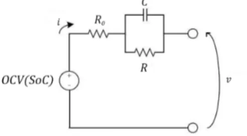
Figure 3-1 shows a typical battery’s voltage response to a discharging square-wave input current waveform. The corresponding output voltage profile has the following three distinct characteristics:

1. A constant voltage at the end of the zero-current transients, which corresponds to the 𝑂𝐶𝑉. As can be seen, the 𝑂𝐶𝑉 decreases with each discharging pulse, manifesting its dependence on the 𝑆𝑜𝐶. This confirms the presence of an ideal voltage source of value 𝑂𝐶𝑉(𝑆𝑜𝐶), given by the 𝑂𝐶𝑉 − 𝑆𝑜𝐶 relation of the battery. The 𝑆𝑜𝐶 is estimated by an external system that then feeds it to the generator.

2. An immediate voltage drop/rise in correspondence with the rising/falling steps of the current pulses, which unveils that the battery is a proper dynamical system. This behaviour can be modelled with a resistor 𝑅M placed in series to the voltage generator.

3. Low-pass transients that immediately follow the voltage steps, which can be modelled by an 𝑅𝐶-parallel also placed in series to 𝑂𝐶𝑉(𝑆𝑜𝐶) and 𝑅M.

From these initial considerations, the basic TM works out to be that shown in Figure 3-2; confirming the TEC structure. The basic TM can be extended and modified to model various other physical phenomena of the battery, which we will now discuss. Negligibly or not, the values of the components introduced depend on the 𝑆𝑜𝐶, 𝑇, and the current. Of which only the first two are examinable by EIS, but only at small values of the current (see section 3.2.2).

Figure 3-1: The voltage profile of a Li-ion cell, corresponding to the outgoing current shown on top. Reprinted from [28].

A cell-model for the multi-cell modelling of battery-packs