POLITECNICO DI MILANO
Scuola di Ingegneria Industriale e dell’Informazione
Dipartimento di Chimica, Materiali e Ingegneria Chimica “Giulio Natta”
Corso di Laurea Magistrale in Ingegneria Chimica
A pharmacokinetic-pharmacodynamic model for
remifentanil administration in anesthesia
Supervisor: prof. Davide MANCA
Master degree thesis of:
Adriana SAVOCA, 837204
Cristina VERGANI, 832889
1
Contents
Figures ... 5 Tables ... 15 Acronyms ... 23 Symbols ... 25 Abstract ... 27 Estratto ... 29 1. INTRODUCTION... 311.1 Research context and objectives of the thesis ... 31
1.2 Pharmacokinetics and pharmacodynamics ... 35
1.2.1 Pharmacokinetics ... 36
1.2.2 Pharmacodynamics ... 41
1.3 Analgesics and anesthesiology ... 43
1.4 Remifentanil... 45
1.4.1 Introduction and physiochemical characteristics ... 45
1.4.2 Mechanism of action... 47
1.4.3 Pharmacokinetics of remifentanil ... 48
1.4.4 Pharmacodynamics of remifentanil ... 49
1.4.5 Clinical uses and dosage ... 51
2. PHARMACOKINETICS ... 53
2.1 Pharmacokinetics modeling: focus on Physiologically Based Pharmacokinetics models ... 53
2.2 Abbiati et al. (2016) PBPK model ... 55
2.3 Six-parameter PK model ... 66
2.4 Model validation and comparison with Abbiati et al. (2016) work ... 69
2.4.1 Case-study 1: Egan et al. (1996) ... 69
2.4.2 Case-study 2: Westmoreland et al. (1993) ... 77
2.4.3 Case-study 3: Pitsiu et al. (2004) ... 79
2.4.4 Case-study 4: Glass et al. (1993) ... 82
2.4.5 Conclusions ... 83
2
2.7.1 Variation of the protein binding ... 88
2.7.2 Saturation of enzymes ... 91
2.7.3 Results and discussion ... 93
2.8 Temperature dependence ... 105
2.8.1 Temperature dependence model ... 107
2.8.2 Results and discussion -Case-study 1: Davis et al. (1999) ... 111
2.8.3 Results and discussion - Case-study 2: Sam et al. (2009) ... 113
2.8.4 Conclusions ... 115
3. PHARMACODYNAMICS ... 117
3.1 Pharmacodynamic modeling of remifentanil ... 117
3.2 Pharmacological effects ... 119 3.2.1 Blood pressure ... 119 3.2.2 Heart rate ... 121 3.2.3 Minute ventilation ... 122 3.2.4 Bispectral index ... 123 3.3 Modeling approach ... 124 3.3.1 𝑀𝐴𝑃 and 𝑆𝐴𝑃 model ... 131 3.3.2 𝐻𝑅 model ... 133
3.4 Results and discussion – 𝑆𝐴𝑃 model ... 138
3.4.1 Case-study 1: Lee et al. (2012) ... 138
3.4.2 Case-study 2: O’Hare et al. (1999) ... 139
3.4.3 Case-study 3: Park et al. (2011) ... 140
3.4.4 Case-study 4: Nora et al. (2007) ... 141
3.4.5 Conclusions ... 142
3.5 Results and discussion – 𝑀𝐴𝑃 model ... 143
3.5.1 Case-study 1: Hall et al. (2000) ... 143
3.5.2 Case-study 2: Alexander et al. (1999) ... 144
3.5.3 Case-study 3: Batra et al. (2004)... 145
3.5.4 Conclusions ... 146
3
3.6.1 Case-study 1: Lee et al. (2012) ... 146
3.6.2 Case-study 2: Park et al. (2011) ... 147
3.6.3 Case-study 3: Nora et al. (2007) ... 147
3.6.4 Case-study 4: Hall et al. (2000) ... 148
3.6.5 Case-study 5: Maguire et al. (2001) ... 149
3.6.6 Case-study 6: Shajar et al. (1999) ... 150
3.6.7 Conclusions ... 150
3.7 Limitations of the PD model ... 151
4. A COMBINED PK-PD MODEL ... 153
4.1 Combined models and effect-site compartment ... 153
4.2 Evaluation of the distribution rate constant 𝑘𝑒0 ... 155
4.3 Application to 𝑆𝐴𝑃 ... 158
4.3.1 Case-study 1: Lee et al. (2012) ... 159
4.3.2 Case-study 2: O’Hare et al. (1999) ... 160
4.3.3 Case-study 3: Park et al. (2011) ... 162
4.3.4 Case-study 4: Nora et al. (2007) ... 163
4.3.5 Conclusions ... 165
4.4 Application to 𝑀𝐴𝑃 ... 165
4.4.1 Case-study 1: Hall et al. (2000) ... 166
4.4.2 Case-study 2: Alexander et al. (1999) ... 167
4.4.3 Case-study 3: Batra et al. (2004) ... 169
4.4.4 Conclusions ... 170
4.5 Application to 𝐻𝑅 ... 171
4.5.1 Case-study 1: Lee et al. (2012) ... 173
4.5.2 Case-study 2: Park et al. (2011) ... 173
4.5.3 Case-study 3: Nora et al. (2007) ... 175
4.5.4 Case-study 4: Hall et al. (2000) ... 176
4.5.5 Case-study 5: Maguire et al. (2001) ... 177
4.5.6 Case-study 6: Shajar et al. (1999) ... 178
4.5.7 Conclusions ... 179
4.6 Effect of the variation of dose and dose regimen ... 180
4
5.2 Pharmacokinetic results... 195
5.2.1 Case-study 1: Egan et al. (1996) ... 195
5.2.2 Case-study 2: Westmoreland et al. (1993) ... 201
5.2.3 Case-study 3: Pitsiu et al. (2004) ... 203
5.2.4 Case-study 4: Glass et al. (1993) ... 205
5.2.5 Final remarks ... 206
5.3 Pharmacodynamic results ... 206
5.3.1 Results for 𝑆𝐴𝑃 ... 207
5.3.2 Results for 𝑀𝐴𝑃 ... 212
5.3.4 Final remarks ... 221
6. CONCLUSIONS AND FUTURE DEVELOPMENTS ... 223
5
Figures
Figure 1 - (A) Rate of approval for FDAs since 1960 (US Food and Drug Administration, 2013), (B) Number of approved drugs for every billion US dollars spent on R&D (Scannel et al., 2012). ... 32 Figure 2 - Schematic representation of the interaction between the pharmacokinetics and the pharmacodynamics of a drug. PK analyses provide the concentration profile associated to the selected dose that can be used for PD analyses, which provide the effect profile, used to define the efficacy and the toxicity of the drug. Adapted from Merck Manual, 1982. ... 35 Figure 3 - Schematization of three mechanisms of transport: passive transport (left), facilitated transport (middle), and active transport (right). In the first case the transport occurs because of the drug concentration gradient across two regions. In the second case a carrier molecule facilitates the transport. The last case is a selective process that occurs with the expenditure of an ATP molecule. Taken from Merck Manual, 1982. ... 36 Figure 4 - Representation of the AUC (Area Under Curve), that in the figure is the colored area. AUC is directly proportional to the total amount of unchanged drug that reaches the systemic circulation. The figure is adapted from Merck Manual, 1982. ... 38 Figure 5 - General schematization of enzymes drug metabolism. Taken from Merck Manual, 1982. ... 39 Figure 6 - Typical metabolic pathway of a lipophilic drug inside the human body. The drug is first metabolized by the liver and then it reaches the kidneys where it is eliminated. Taken from Merck Manual, 1982. ... 40 Figure 7 - Interaction between a drug and its specific receptor. The pharmacological effect is explicated through this interaction. Taken from Merck Manual, 1982. ... 41 Figure 8 - Mechanisms of action of both agonists and antagonists. Taken from Merck Manual, 1982. ... 43 Figure 9 - Chemical structure of morphine. ... 44 Figure 10 - Chemical structure of remifentanil. (Left) The atoms are represented as spheres. White spheres are hydrogen, grey are carbon, blue are nitrogen, and red are oxygen. ... 47
6
Figure 12 - Classical three-compartment pharmacokinetic model. The central compartment represents the plasma, while the side compartments represent the highly perfused organs/tissues (Rapidly equilibrating Compartment) and poorly perfused organs/tissues (Slowly equilibrating Compartment). ... 53 Figure 13 - Representation of Teorell's model (1937). Taken from Reddy et al. (2005). . 54 Figure 14 - Representation of Abbiati et al. (2016) model composed of eight compartments: GL (Gastric Lumen), SIL (Small Intestinal Lumen), LIL (Large Intestinal Lumen), GICS (Gastro-Intestinal Circulatory System), Liver, Plasma, PT (Poorly Perfused Tissues) and HO (Highly Perfused Organs). In addition, the material flows between the different compartments are represented with black arrows. Red arrows show the elimination paths and purple dashed arrows the possible administration paths. Taken from Abbiati et al. (2016). ... 56 Figure 15 - Schematic representation of the minimized model for remifentanil. GL, LIL, and SIL are neglected because remifentanil is an intravenous administered drug. Taken from Abbiati et al. (2016). ... 66 Figure 16 - Schematization of the six-parameter model. The hepatic and renal clearances can be neglected. Adapted from Abbiati et al. (2016). ... 68 Figure 17 - Experimental data (red) from Egan et al. (1996). Ten volunteers were administered increasing doses of remifentanil with a 20 min infusion. The left portion shows the results of the 8P model (blue) from Abbiati et al. (2016), whilst the right portion the results of the 6P model (blue). It is possible to see that moderately better results are obtained with the 6P model. ... 73 Figure 18 - Experimental data (red) from Westmoreland et al. (1993). Four groups of patients were administered with four boluses over 60 s. On the left the results of the 8P model (blue) from Abbiati et al. (2016), on the right the results of the 6P model (blue).78 Figure 19 - Experimental data of four patients administered with a dose of 6-9 μg/kg/h for 72 h (Pitsiu et al., 2004). Left side, results of the 8P model (blue) of Abbiati et al.
7 (2016). Right side, results of the 6P model (blue). It is possible to observe that the 6P model produces moderately better results. ... 81 Figure 20 - Experimental data (red) of 30 volunteers administered with a single bolus for 60 s (Glass et al., 1993). Left side, the results of the 8P model (blue) of Abbiati et al. (2016). Right side, results from the 6P model (blue). It is possible to see that the 6P model produces moderately better results. ... 82 Figure 21 - Comparison between the 6P model (blue) and the experimental data (red) of Patient 1 from Navapurkar et al. (1998). It is evident that the model overestimates the peak of the blood concentration of remifentanil. ... 85 Figure 22 - Measured blood concentrations of Patient 1 during the dissection (hepatic) and anhepatic phases. ... 85 Figure 23 - Measured blood concentrations of healthy (red) and renal-failure (blue) patients from Dahaba et al. (1998). It is possible to detect a difference in the pharmacokinetics between healthy and sick patients. ... 86 Figure 24 - Comparison between the 6P model and the experimental data of Dahaba et al. (1998). It is evident that the model underestimates the experimental data. ... 87 Figure 25 - Trend of the experimental and model maximum concentration of remifentanil for increasing dose (experimental Cmax (red) from Egan et al., 1993). It is
possible to observe a linear trend for doses up to 2 μg/kg. For higher doses the model Cmax (blue) deviates from the experimental data. ... 88
Figure 26 - Structure of alpha-1-acid glycoprotein, taken from Tesseromatis et al. (2011). ... 89 Figure 27 - Trend of the rate of a reaction catalyzed by enzymes, in response to the variation of the substrate and enzymes concentrations. (Source: UW (University of Washington) Departments web server). ... 92 Figure 28 - Experimental data (red) from Egan et al. (1993). The left portion shows the results of the 6P model (blue). The right portion shows the results of the 6P Binding model (blue). It is possible to see that better results are obtained with the 6P Binding model. ... 97
8
mode (blue). It is possible to see that better results are obtained with the 6P Enzymes model. ... 102 Figure 30 - (Left) Results of the penalty function method. (Right) Results of the constrained optimization. Experimental data (red) of Davis et al. (1999). ... 111 Figure 31 - Simulation of a virtual patient administered with two boluses of remifentanil. ... 113 Figure 32 - Experimental data (red) of Patient 1 and 2 from Sam et al. (2009). On the left the penalty function method results, on the right the constrained optimization results. ... 114 Figure 33 - Generic trend of ECG (top). Heart anatomy (bottom). Taken from the American Heart Association. ... 122 Figure 34 - Experimental data from Hall et al. (2000). (Top) Experimental SAP. (Middle) Experimental MAP. (Bottom) Experimental HR. Standard deviation bars provide a measure of the inter-individual variability. The peak that can be detected at 4.5 min is due to the cardiovascular stress response of the patient to intubation and laryngoscopy. ... 126 Figure 35 - Comparison between the experimental data (red) of Group 1 of O’Hare et al. (1999) and the simulation with the sigmoidal Emax model (blue). The patient received 0.5
μg/kg over 30 s. The model does not represent the stress response to intubation. ... 131 Figure 36 - Experimental HR from Group 1 and 2 of Hall et al. (2000), minus the first peak. ... 134 Figure 37 - Experimental data (red) of O'Hare et al. (1999). The blue line is the modified Emax model overestimated with the 1st order response. The concavity is opposite respect
to the one of the experimental data. ... 136 Figure 38 - Comparison between the PD model (blue) and the experimental data (red) of Group 1 from Lee et al. (2012). ... 138 Figure 39 - Comparison between the PD model (blue) and the experimental data (red) of Group 1, 2, and 3 from O'Hare et al. (1999). ... 140
9 Figure 40 - Comparison between the PD model (blue) and the experimental data (red) of Group 1 and 2 from Park et al. (2011). ... 141 Figure 41 - Comparison between the PD model (blue) and the experimental data (red) of Group 1 and 2 of Nora et al. (2007). ... 142 Figure 42 - Comparison between the PD model (blue) and the experimental data (red) of Group 1 and 2 from Hall et al. (2000). ... 143 Figure 43 - Comparison between the PD model (blue) and the experimental data (red) of Group 1, 2, and 3 from Alexander et al. (1999). ... 144 Figure 44 - Comparison between the PD model (blue) and the experimental data (red) of Group 1 and 2 from Batra et al. (2004). ... 145 Figure 45 - Comparison between the PD model (blue) and the experimental data (red) of Group 1 of Lee et al. (2012). ... 146 Figure 46 - Comparison between the PD model (blue) and the experimental data (red) of Group 1 and 2 from Park et al. (2011). ... 147 Figure 47 - Comparison between the PD model (blue) and the experimental data (red) from Nora et al. (2007). ... 148 Figure 48 - Comparison between the PD model (blue) and the experimental data (red) of Group 1 and 2 from Hall et al. (2000). ... 148 Figure 49 - Comparison between the PD model (blue) and the experimental data (red) of Group1 from Maguire et al. (2001). ... 149 Figure 50 - Comparison between the PD model (blue) and the experimental data (red) of Group 1 from Shajar et al. (1999). ... 150 Figure 51 - Anticipation of the model in the prediction of the effect respect to the experimental data. Experimental MAP (red) of Group 1 and 2 from Hall et al. (2000) study. ... 151 Figure 52 - Schematic representation of a combined PK-PD model. The effect-site compartment connects the PK model to the PD model. ... 154 Figure 53 - On the left, dynamic evolution of the plasma concentration and the effect in time. It is possible to detect a delay between the peak concentration and the peak effect. On the right, the hysteresis loop between the effect and the plasma
10
Figure 54 - Comparison between the simulated concentration-time profiles in the plasma (red) and effect-site (blue) compartment. ... 157 Figure 55 - The left figure shows the hysteresis loop before the optimization procedure. The right figure shows the collapsed hysteresis loop after the optimization procedure. Experimental data (red) from Maguire et al. (2001). ... 158 Figure 56 - On the left, the results of the PD model. On the right, the results of the combined 6P PK-PD model. Experimental data come from Lee et al. (2012). The administered dose was 1 µg/kg as a single bolus over 1 min. ... 159 Figure 57 - The left portion shows the results of the PD model. The right portion shows the results of the combined model. Experimental data come from O’ Hare et al. (1999). The patients were divided in three groups and received increasing doses as single bolus over 30 s. ... 161 Figure 58 - The left portion shows the results of the PD model. The right portion shows the results of the combined model. Experimental data from Park et al. (2011). The patients were divided in two groups and received two different doses as single bolus over 30 s. ... 162 Figure 59 - The left portion shows the results of the PD model. The right portion shows the results of the combined model. Experimental data come from Nora et al. (2007). The difference between the groups is the time at which the remifentanil administration start ... 164 Figure 61 - The left portion shows the results of the PD model. The right portion shows the results of the combined model. Experimental data (red) from Hall et al. (2000). The patients were divided in two groups and received two different doses as single bolus for 30 s followed by an IV infusion. ... 166 Figure 62 - The left portion shows the results of the PD model. The right portion shows the results of the combined model. Experimental data come from Alexander et al. (1999). The patients were divided into three groups and received three different doses as single bolus for 10 s. ... 168
11 Figure 63 - The left portion shows the results of the PD model. The right portion shows the results of the combined model. Experimental data come from Batra et al. (2004). The patients were divided into two Groups and received two different doses as single bolus for 30 s. ... 170 Figure 64 - The left portion shows the hysteresis loop before the optimization procedure. The right portion shows the collapsed hysteresis loop after the optimization procedure. Experimental data (red) from O'Hare et al. (1999). ... 172 Figure 65 - On the left, the results of the PD model. On the right, the results of the combined model. Experimental data (red) from Lee et al. (2012). The patients received a single bolus over 1 min. ... 173 Figure 66 - The left portion shows the results of the PD model. The right portion shows the results of the combined model. Experimental data (red) from Park et al. (2011). The patients were divided in two groups and received two different doses as single bolus for 30 s. ... 174 Figure 67 - The left portion shows the results of the PD model. The right portion shows the results of the combined model. Experimental data from Nora et al. (2007). The difference between the groups is the time at which the remifentanil administration starts. The IV infusion starts at time 0 for Group 1 and after 2 min for Group 2. ... 175 Figure 68 - The left portion shows the results of the PD model. The right portion shows the results of the combined model. Experimental data (red) from Hall et al. (2000). The patients were divided into two groups and received two different doses as single bolus for 30 s followed by IV infusion. ... 177 Figure 69 - The left portion shows the results of the PD model. The right portion shows the results of the combined model. Experimental data (red) from Maguire et al. (2001). The patients received a single bolus for 30 s followed by IV infusion. ... 178 Figure 70 - The left side shows the results of the PD model. The right side shows the results of the combined 6P PK-PD model. Experimental data (red) from Shajar et al. (1999). The patients received a single bolus for 30 s. ... 179
12
increasing dose. ... 181 Figure 72 - HR evolution in time in the phase that immediately follows remifentanil administration. ... 181 Figure 73 - Plasma concentration evolution in time and hemodynamic effects resulting from the administration of four different doses as IV infusion. The arrow shows the direction of increasing dose. ... 183 Figure 74 - HR evolution in time in the phase that immediately follows remifentanil administration. ... 184 Figure 75 - Plasma concentration evolution in time and hemodynamic effects resulting from the administration of three different bolus doses. The arrow shows the direction of increasing dose. ... 185 Figure 76 - Comparison between PK and PD of a male patient (red) and a female patient (blue) to investigate the influence of the gender. ... 187 Figure 77 - Concentration-time profile for patients with increasing body weight. On the right, we focus on the two patients with the most extreme conditions and one normweight patient. ... 189 Figure 78 - Concentration-time profile of remifentanil in the poorly perfused tissues, highly perfused organs, liver, and GICS. Comparison of patients with different body weight: obese, normweight and underweight. ... 191 Figure 79 - Influence of the body weight on the hemodynamic effects. The right portion focuses on the phase that follows remifentanil administration.. ... ………192 Figure 80 - Structure of the three-compartment model, adapted from Minto et al. (1997). ... 194 Figure 81 - The left portion shows the results of the 6P model. The right portion shows the results of the 3-compartment PK model of Minto et al., 1997. The experimental data (red) are from Egan et al. (1996). ... 198
13 Figure 82 - The left portion shows the results of the 6P model. The right portion shows the results of the 3-compartment PK model of Minto et al., 1997. The experimental data are from Westmoreland et al. (1993). ... 202 Figure 83 - The left portion shows the results of the 6P model. The right portion shows the results of the 3-compartment PK model of Minto et al., 1997. The considered experimental data (red) are from Pitsiu et al. (2004). ... 204 Figure 84 - The left figure shows the results of the 6P model. The right figure shows the results of the 3-compartment PK model of Minto et al., 1997. The experimental data (red) are from Glass et al. (1993). ... 205 Figure 85 - The left figure shows the results of the 6P PK-PD model. The right figure shows the results of the 3-compartment PK-PD model. The experimental data (red) are from Lee et al. (2012). ... 207 Figure 86 - The left portion shows the results of the 6P PK-PD model. The right portion shows the results of 3-compartment PK-PD model. The experimental data (red) are from Park et al. (2011). ... 209 Figure 87 - The left portion shows the results of the 6P PK-PD model. The right portion shows the results of the 3-compartment PK-PD model. The experimental data (red) are from O'Hare et al. (1999). ... 211 Figure 88 - The left portion shows the results of the 6P PK-PD model. The right portion shows the results of the 3-compartment PK-PD model. The experimental data (red) are from Alexander et al. (1999). ... 213 Figure 89 - The left portion shows the results of the 6P PK-PD model. The right portion shows the results of the 3-compartment PK-PD model. The experimental data (red) are from Hall et al. (2000). ... 215 Figure 90 - The left portion shows the results of the 6P PK-PD model. The right portion shows the results of the 3-compartment PK-PD model. The experimental data (red) are from Batra et al. (2004). ... 216 Figure 91 - The left figure shows the results of the 6P PK-PD model. The right figure shows the results of the 3-compartment PK-PD model. The considered experimental data (red) are from Lee et al. (2012). ... 217
14
from Park et al. (2011). ... 219 Figure 93 - The left figure shows the results of the 6P PK-PD model. The right figure shows the results of the 3-compartment PK-PD model. The experimental data (red) are from Maguire et al. (2001). ... 220 Figure 94 - Schematic representation of the in silico anesthesia control-loop. The set point is a target effect. The MP controller generates a control action as IV infusion rate. The 6P PK-PD model is used to simulate a virtual patient. The classical three-compartment... 225 Figure 95 - Schematic representation of the in vivo anesthesia control-loop. The set point is a target effect. The controller generates a control action as IV rate of infusion, employing the 6P PK-PD model. The real patient is represented by a laboratory mouse. ... 226 Figure 96 - TCI pump (Taken from Gopinath et al., 2015). ... 227
15
Tables
Table 1 - Comparison of some of the most important pharmacokinetic parameters of three drugs belonging to the fentanyl family: alfentanil, fentanyl, and remifentanil. Values from Glass et al. (1999) ... 46 Table 2 - Recommended doses of some important drugs in anesthesiology. Source: Injection Prescribing Information by Mylan. ... 51 Table 3 - Parameters of the model that can be categorized into: individualized, assigned, or degrees of freedom ... 61 Table 4 - Body mass fraction and density of different organs and tissues (Brown et al., 1997) ... 64 Table 5 - From the left: lower bounds for the constrained optimization, initial values of the model parameters, upper bounds for the constrained optimization, final optimized values derived from the parameter identification procedure . ... 69 Table 6A - Compariso of ΔCmax% values for the patients of Egan et al. (1996). Left
column, ΔCmax% values for the 8P model of Abbiati et al. (2016). Right column, ΔCmax%
values for the 6P model. ... 74 Table 6B - Comparison of ΔAUC values for the patients of Egan et al. (1996). Left column, ΔAUC values for the 8P model of Abbiati et al. (2016). Right column, ΔAUC values for the 6P model ... 75 Table 6C - Comparison of SAE values for the patients of Egan et al. (1996). Left column, SAE values for the 8P model of Abbiati et al. (2016). Right column, SAE values for the 6P model ... 76 Table 6D - Comparison of IAE values for the patients of Egan et al. (1996). Left column, IAE values for the 8P model of Abbiati et al. (2016). Right column, IAE values for the 6P model... 76 Table 7A - Comparison of ΔCmax% values for the patients of Westmoreland et al. (1993).
Left column, ΔCmax% values for the 8P model of Abbiati et al. (2016). Right column,
16
for the 6P model... 79 Table 7C - Comparison of IAE values for the patients of Westmoreland et al. (1993). Left column, IAE values for the 8P model of Abbiati et al. (2016). Right column, IAE values for the 6P model... 79 Table 8A - Comparison of SAE values for the patients of study of Pitsiu et al. (2004). Left column, SAE values for the 8P model of Abbiati et al. (2016). Right column, SAE values for the 6P model... ... 81 Table 8B- Comparison of IAE values for the patients of study of Pitsiu et al. (2004). Left column, IAE values for the 8P model of Abbiati et al. (2016). Right column, IAE values for the 6P model... ... 81 Table 9A - Comparison of SAE values for the patients of study of Glass et al. (1993). Left column, SAE values for the 8P model of Abbiati et al. (2016). Right column, SAE values for the 6P model... ... 82 Table 9B - Comparison of IAE values for the patients of study of Glass et al. (1993). Left column, values for the Abbiati et al. (2016) model. Right column, values for the 6P model... 82 Table 10 - AIC values for the two models. It is possible to notice that the value is lower for the 6P model... 84 Table 11A - Comparison of ΔCmax% values between the models. Left column, values of
the 6P model. Right column,values of the 6P Binding model... . 97 Table 11B - Comparison of IAE values between the models. Left column, values of the 6P model. Right column,values of the 6P Binding model... . 98 Table 11C - Comparison of SAE values between the models. Left column, values of the 6P model. Right column,values of the 6P Binding model... .. 98 Table 12A - Comparison of ΔCmax% values between the models for Egan et al. (1996).
Left column, values of the 6P model. Right column,values of the 6P Enzymes model... 102 Table 12B - Comparison of IAE values between the models for Egan et al. (1996). Left column, values of the 6P model. Right column,values of the 6P Enzymes model... 103
17 Table 12C - Comparison of SAE values between the models for Egan et al. (1996). Left
column, values of the 6P model. Right column,values of the 6P Enzymes model... 103
Table 13 - Values of the performance indexes. Comparison between the 6P Enzymes and the 6P Binding model. ... ...104
Table 14 - Initial values of the model parameters. Second column, lower bounds of the parameters, Fourth column, upper bounds of the parameters...109
Table 15 - Final values of the parameters of the model. Left column, values from the application of the penalty function method. Right column, values from the constrained optimization routine. ... ...111
Table 16 - Comparison of ΔCmax%, SAE, and IAE values between the set of parameters. Left column, values for the penalty function method. Right column, values for the constrained optimization. ... ...112
Table 17 - Average administered infusion rates throughout the three phases of the operation (Sam et al., 2009) ... 114
Table 18 - Comparison of the values of performance indexes between the set of parameters. Left column, values for the penalty function method. Right column, values for the constrained optimization... 115
Table 19 - Ranges for systolic and diastolic pressures. Source: American Heart Association... 120
Table 20A - Time required to reach the SAP peak ... 127
Table 20B -Time required to reach the MAP peak ... 127
Table 20C - Time required to reach the HR peak... 127
Table 21A - Percentage of increase for SAP ... 128
Table 21B - Percentage of increase for MAP ... 128
Table 21C - Percentage of increase for HR... 129
Table 22A - Time required for the decrease of SAP ... 129
Table 22B - Time required for the decrease of MAP... 130
Table 22C - Time required for the decrease of HR... 130
Table 23A - Adaptive parameters details of SAP model... 133
18
Table 25 - ΔEmax % and SAE values for Group 1,2, and 3 of O’Hare et al. (1999)... 140
Table 26 - ΔEmax % and SAE values for Group 1 and 2 of Park et al. (2011)... 141
Table 27 - ΔEmax % and SAE values for Group 1 of Nora et al. (2007)... 142
Table 28 - ΔEmax % and SAE values for Group 1 and 2 of Hall et al. (2000)... 143
Table 29 - ΔEmax % and SAE values for Group 1,2, and 3 of Alexander et al. (1999)... 145
Table 30 - ΔEmax % and SAE values for Group 1 and 2 of Batra et al. (2004)... 146
Table 31 - ΔEmax % and SAE values for Group 1 of Lee et al. (2012)... 147
Table 32 - ΔEmax % and SAE values for Group 1 and 2 of Park et al. (2011)... 147
Table 33 - ΔEmax % and SAE values for Group 1 and 2 of Nora et al. (2007)... 148
Table 34 - ΔEmax % and SAE values for Group 1 and 2 of Hall et al. (2000)... 149
Table 35 - ΔEmax % and SAE values for Group 1 of Maguire et al. (2001)... 149
Table 36 - ΔEmax % and SAE values for Group 1 of Shajar et al. (1999)...150
Table 37 - Values of the performance indexes for Lee et al. (2012). Left column, values for PD model. Right column, values for 6P PK-PD model... 159
Table 38 - Values of the performance indexes for O’Hare et al. (1999). Left column, values for PD model. Right column, values for 6P PK-PD model... 161
Table 39 - Values of the performance indexes for Park et al. (2011). Left column, values for PD model. Right column, values for 6P PK-PD model... 163
Table 40 - Values of the performance indexes for Nora et al. (2007). Left column, values for PD model. Right column, values for 6P PK-PD model... 164
Table 41 - Values of the performance indexes for Hall et al. (2001). Left column, values for PD model. Right column, values for 6P PK-PD model... 167
Table 42 - Values of the performance indexes for Alexander et al. (1999). Left column, values for PD model. Right column, values for 6P PK-PD model... 169
Table 43 - Values of the performance indexes for Batra et al. (2004). Left column, values for PD model. Right column, values for 6P PK-PD model... 170
Table 44 - Values of the performance indexes for Lee et al. (2012). Left column, values for PD model. Right column, values for 6P PK-PD model... 173
19 Table 45 - Values of the performance indexes for Park et al. (2011). Left column, values for PD model. Right column, values for 6P PK-PD model... 174 Table 46 - Values of the performance indexes for Nora et al. (2007). Left column, values for PD model. Right column, values for 6P PK-PD model... 176 Table 47 - Values of the performance indexes for Hall et al. (2000). Left column, values for PD model. Right column, values for 6P PK-PD model...177 Table 48 - Values of the performance indexes for Maguire et al. (2001). Left column, values for PD model. Right column, values for 6P PK-PD model... 178 Table 49 - Values of the performance indexes for Shajar et al. (1999). Left column, values for PD model. Right column, values for 6P PK-PD model... 179 Table 50 - Demographic data of the simulated patients and administered bolus doses... 180 Table 51 - Demographic data of the simulated patients and administered infusion doses... 182 Table 52 - Demographic data of the simulated patients and administered doses... 184 Table 53 - Demographic data of the simulated patients...186 Table 54 - Classification of the condition, depending on the BMI. Taken from Domi and Laho (2012)……...188 Table 55 - Demographic data and BMI of the simulated patients. Last column, administered doses………...188 Table 56 - LBM and BMI of the simulated patient ... 190 Table 57 - Values of the parameters of the 3-compartment PK model for remifentanil, taken from Minto et al. (1997)... 195 Table 58A - Comparison of the ∆Cmax% values between the 6P and Minto’s models
based on Egan et al. (1996) experimental data... 199 Table 58B - Comparison of the SAE values between the 6P and Minto’s models based on Egan et al. (1996) experimental data... 199 Table 58C - Comparison of the IAE values between the 6P and Minto’s models based on Egan et al. (1996) experimental data... 200
20
Table 59B - Comparison of the SAE values between the 6P and Minto’s models based on Westmoreland et al. (1993) experimental data...202 Table 59C - Comparison of the IAE values between the 6P and Minto’s models based on Westmoreland et al. (1993) experimental data...203 Table 60A - Comparison of the SAE values between the 6P and Minto’s models based on Pitsiu et al. (2004) experimental data...205 Table 60B - Comparison of the IAE values between the 6P and Minto’s models based on Pitsiu et al. (2004) experimental data...205 Table 61 - Comparison of the SAE and IAE values between the 6P and Minto’s models based on Glass et al. (1993) experimental data...206 Table 62 - Left column, values of 𝑘𝑒0 for the 6P PK-PD model. Right column, values for
the 3-compartment PK-PD model... 207 Table 63 - Comparison of ∆Emax% and SAE values for SAP between the 6P PK-PD and
Minto’s PK-PD models based on Lee et al. (2012) experimental data…... 208 Table 64A - Comparison of the ∆Emax% values between the 6P PD and Minto’s
PK-PD SAP models based on Park et al. (2011) experimental data... 209 Table 64B - Comparison of the 𝑆𝐴𝐸 values between the 6P PK-PD and Minto’s PK-PD SAP models based on Park et al. (2011) experimental data... 209 Table 65A - Comparison of the ∆𝐸𝑚𝑎𝑥% values between the 6P PD and Minto’s PK-PD SAP models based on O’Hare et al. (1999) experimental data...211 Table 65B - Comparison of the 𝑆𝐴𝐸 values between the 6P PK-PD and Minto’s PK-PD SAP models based on O’Hare et al. (1999) experimental data... 211 Table 66A - Comparison of the ∆𝐸𝑚𝑎𝑥% values between the 6P PD and Minto’s
PK-PD MAP models based on Alexander et al. (1999) experimental data... 213 Table 66B - Comparison of the 𝑆𝐴𝐸 values between the 6P PK-PD and Minto’s PK-PD MAP models based on Alexander et al. (1999) experimental data... 214 Table 67A - Comparison of the ∆𝐸𝑚𝑎𝑥% values between the 6P PD and Minto’s
21 Table 67B - Comparison of the 𝑆𝐴𝐸 values between the 6P PK-PD and Minto’s PK-PD MAP models based on Hall et al. (2000) experimental data...215 Table 68A - Comparison of the ∆𝐸𝑚𝑎𝑥% values between the 6P PD and Minto’s
PK-PD MAP models based on Batra et al. (2004) experimental data...216 Table 68B - Comparison of the 𝑆𝐴𝐸 values between the 6P PK-PD and Minto’s PK-PD MAP models based on Batra et al. (2004) experimental data... 217 Table 69 - Comparison of the ∆Emax% and SAE values between the 6P PK-PD and
Minto’s PK-PD HR models based on Lee et al. (2012) experimental data... 218 Table 70A - Comparison of the ∆Emax% values between the 6P PD and Minto’s
PK-PD 𝐻𝑅 models based on Park et al. (2011) experimental data... 219 Table 70B - Comparison of the 𝑆𝐴𝐸 values between the 6P PK-PD and Minto’s PK-PD 𝐻𝑅 models based on Park et al. (2011) experimental data... 219 Table 71 - Comparison of the ∆Emax% and SAE values between the 6P PK-PD and
23
Acronyms
ADME Absorption, Distribution, Metabolism, and Excretion
AGP Alpha-1-acid GlycoProtein
AIC Akaike Information Criterion
AP Arterial Pressure
ATP Adenosine Triphosphate
AUC Area Under Curve
BIS Bispectral Index
BMI Body Mass Index
CPB CardioPulmonary Bypass
CSF CerebroSpinal Fluid
CSTR Continuously Stirred Tank Reactor
DAP Diastolic Arterial Pressure
E Effect
ECG ElectroCardioGraphy
EEG ElectroEncephaloGram
FDA Food and Drug Administration
GICS Gastro-Intestinal Circulatory System
GL Gastric Lumen
HO Highly perfused Organs
HR Heart Rate
IAE Integral of the Absolute Error
ICU Intensive Care Unit
24
ODE Ordinary Differential Equation
OLT Orthopic Liver Transplantation
PD PharmacoDynamics
PDE Partial Differential Equation
PFR Plug Flow Reactor
PK PharmacoKinetics
PT Poorly perfused Tissues
QSP Quantitative Systems Pharmacology
R&D Research and Development
RA Remifentanil Acid
RR Respiratory Rate
SAE Sum of Absolute Errors
SAP Systolic Arterial Pressure
SIL Small Intestinal Lumen
SSE Sum of Squared Error
TCI Target Controlled Infusion
TIVA Total Intravenous Anesthesia
UK United Kingdom
USA United States of America
25
Symbols
𝐵𝑀 Body Mass [kg]
𝐵𝑆𝐴 Body Surface Area [m2]
𝐶 Drug Concentration [ng/mL]
𝐶𝐿 Clearance [mL/min]
𝐶𝑂 Cardiac Output [L/min]
𝐸𝑓𝑓 Efficiency -
𝐹 Material Flux [ng/mL/min]
𝐹𝑟 Fraction -
ℎ Height [cm] or [m]
𝐼𝑉 Intra Venous dose [ng/min]
𝐾 Mass transfer coefficient [min-1]
M Body mass [kg]
𝑃𝑂 Drug orally administered [ng/min]
𝑄 Plasmatic fraction of blood [mL/min]
𝑅 Protein binding -
𝜌 Density [g/mL]
𝑡 Time [min]
𝑡1 2
⁄ 𝛽 Half-time elimination [min]
𝑡1 2
⁄ 𝑘𝑒0 Half-life for equilibration [min]
𝑉 Volume [cm3] or [mL]
𝑉𝑑,𝑠𝑠 Steady state volume of
distribution
27
Abstract
Today, anesthesiologists’ role is extremely difficult, as there is neither a precise definition of the anesthetic state nor a standard measurement to evaluate analgesia. Furthermore, the optimal analgesic dose must both grant safe conditions and account for the patient features. Therefore, pharmacokinetic-pharmacodynamic (PK-PD) models are growing in importance. Among analgesic opioids used in anesthesia, remifentanil features a short-range action.
Our target is the development of a PK-PD model for remifentanil administration in anesthesia. The reference work is the physiologically-based (PB) PK model of Abbiati et al. (2016). Detailed literature investigations led us to neglect two metabolic pathways (i.e. kidneys and liver) that are not involved in remifentanil elimination. To predict the PK at high doses we suggest a protein binding mechanism and a dose-elimination dependence. We propose an Arrhenius-type correlation between the elimination rate constants and body temperature. PD models are usually developed to correlate plasma concentration and the corresponding hemodynamic effects, but they do not describe the physiological delay between plasma concentration and effect. To overcome this problem we added an effect-site compartment. The resulting PK-PD model is used to study different regimens and the gender/weight influence. Finally, we compare our model and the three-compartment PK-PD model, the most used in the literature.
Our model shows better results, being closer to the real metabolic processes. It is also successful in predicting the PK at high doses but the mechanism behind remains unknown. We also validate the temperature dependence model. Adding the effect-site compartment, we get an accurate prediction of the hemodynamic effects in all the anesthesia phases, and achieve an improvement in the PK prediction respect to the classical PK-PD model.
We demonstrate that our model is a suitable tool for the selection of optimal dose regimen, which is still an open issue in anesthesia. As it is able to discriminate among patients, it can be a starting point for the use of personalized formulae to overcome inter-individual variability.
29
Estratto
Il ruolo dell’anestesista è estremamente difficile, poiché non esiste una definizione precisa dello stato anestetico, nè misure standard dell’azione analgesica. La dose ottimale di analgesico deve garantire condizioni sicure e tener conto delle caratteristiche fisiche dei pazienti. In questo contesto diventano importanti i modelli farmacocinetici-farmacodinamici (PK-PD). Tra gli oppioidi analgesici usati in anestesia abbiamo scelto il remifentanil per il suo rapido onset e offset.
Scopo di questo lavoro è costruire un modello PK-PD per la somministrazione del remifentanil in anestesia. Il punto di partenza è il modello PK su base fisiologica di Abbiati et al. (2016). In accordo con la letteratura, abbiamo trascurato due vie metaboliche non coinvolte nell’eliminazione del farmaco. Per predire la PK ad alte dosi abbiamo proposto una dipendenza del legame proteico e dell’eliminazione dalla dose. Abbiamo poi ipotizzato una relazione di tipo Arrhenius tra le costanti di eliminazione e la temperatura corporea. Abbiamo sviluppato modelli PD per legare la concentrazione plasmatica ai corrispondenti effetti emodinamici, che però non rappresentavano il delay che esiste tra concentrazione ed effetto. Il problema è stato superato integrando un effect-site compartment. Il modello PK-PD è stato usato per studiare l’effetto di diverse dosi e posologie e del sesso/massa. Infine, abbiamo confrontato il nostro modello e il modello tri-compartimentale PK-PD, il più diffuso.
Essendo più vicino al reale processo metabolico, il nostro modello ha prodotto risultati migliori. Anche se il meccanismo dietro il trend dei dati per alte dosi rimane non chiaro, il modello riesce a descriverli. Il modello che propone la dipendenza dalla temperatura è stato convalidato. Con l’aggiunta dell’effect-site compartment il modello riesce a predire gli effetti emodinamici durante l’intera anestesia. Rispetto al modello classico, il nostro comporta un avanzamento nella predizione della PK.
Il modello proposto è un valido strumento per la scelta della dose ottimale. Inoltre, essendo sensitivo alle caratteristiche fisiche, può essere un punto di partenza per approfondire terapie individualizzate.
Introduction
31
1. INTRODUCTION
1.1 Research context and objectives of the thesis
The development of quantitative computer modeling of biological systems and the study of drugs pharmacokinetics and pharmacodynamics is today of growing importance to biomedical research.
This is confirmed by the 2011 publication of a white paper by NIH (National Health Institute, USA) concerning the institution of a new discipline: Quantitative Systems Pharmacology (Leil and Ermakov, 2015).
QSP consists of the integration of two disciplines:
(i) Systems biology, aimed at studying the relationship between genes and biologically active molecules in order to develop qualitative models of these systems;
(ii) Quantitative pharmacology, focused on computer-aided modeling and simulation to increase the understanding of the pharmacokinetics and pharmacodynamics of drugs.
In the past, the approach to drug discovery was based on the empirical evidences from nature. This approach was renamed ‘Pharmacognosy’ by a German scientist, C.A. Seydler, who used the word ‘pharmakognosie’ for the first time in 1815 in his book titled “Analecta pharmacognostica”, by merging two Greek words: “pharmakon” (φάρμακον), which means drug and “gignosco” (γιγνώσκω) which means acquiring knowledge.
This approach originates in Egypt and India: medicines were recorded in the Egyptian papyrus about 1500 BC and later in the Indian “Ajur veda” (meaning “Science of Life”). Later, Ancient Rome also promoted the development of drug discovery: in about 77 AD, Dioscorides, a Greek military physician and pharmacognosist of Nero’s army, recorded about 600 kinds of crude drugs in his book “De materia medica”. This book played an important role in the pharmacology and botany of crude drugs in the 15th century. Pliny
the Elder (23-79 AD), contemporary of Dioscorides, gave a brief account in his “Hystoria” of nearly 1000 species of plants, most of which could be used as medicines. Throughout the Middle Age, European physicians referred to the Arab works “De Re Medica” by John Mesue (850 AD), “Canon Medicinae” by Avicenna (980-1037), and “Liber Magnae Collectionis Simplicum Alimentorum Et Medicamentorum” by Ibn Baitar (1197-1248), in which over 1000 medicinal plants were described. In 18th century, in his work Species
Plantarium (1753), Linnaeus (1707-1788) provided a brief description and classification of the species described until then. Later, early 19th century was a turning point in the
knowledge and use of medicinal plants. The discovery and isolation of alkaloids from poppy (1806), ipecacuanha (1817), strychnos (1817), quinine (1820), pomegranate
32
(1878), and other plants, then the isolation of glycosides, marked the beginning of scientific pharmacy. With the improvement of the chemistry, other substances from medicinal plants were also discovered such as hormones and vitamins (Petrovska, 2012). Since the middle of the last century, due to the advances in biochemical and medical sciences, drug discovery has evolved from the empirical approach to a new hypothesis-driven and mechanism-based approach. This has led to two apparently contrasting effects that can be detected starting from the ‘60s: an increase of the percentage of new drug applications approved by FDA (Food and Drug Administration, USA) (Fig.1 A) and, at the same time, a decline in the productivity of drugs (Fig. 1 B).
Figure 1- (A) Rate of approval for FDAs since 1960 (US Food and Drug Administration, 2013), (B) Number of approved drugs for every billion US dollars spent on R&D (Scannel et al., 2012).
This second effect of the modern approach is due to the difficulty of finding new therapeutic targets and to the increase in the costs associated with the discovery and the development of new drugs. This is a typical consequence of any new industry: in order to limit this effect, it is necessary to find strategies that allow increasing the probability of commercial success of the product, and at the same time decrease the development costs (Leil and Bertz, 2014).
Computer-aided modeling is the appropriate solution for both these goals. In fact, computer simulations enable to test a very high number of situations in silico: this means that it is possible to establish the probability of failure of a drug without performing real clinical tests, which are highly expensive. Another important and related advantage is that it is possible to predict the effects of multiple therapeutic interventions in combination, whose testing in the clinic would be in most cases economically and practically unfeasible.
Moreover, QSP models are based on the understanding of the biological pathways, the disease processes, and the drug mechanisms of action. Therefore, they are effective tools for integration of biological knowledge and formulation of pharmacological hypotheses, can aid in pre-clinical and clinical experiments design, and they can provide
Introduction
33 a support for a better insight on the interaction between drugs and biological systems, which is essential in the target identification stage.
For all these reasons, it is possible to claim that QSP allows facing the growing challenges in efficiency and productivity for Research & Development (R&D) of drugs. Given this, it is worth discussing the reasons why the pharmaceutical industry has been slow to integrate computer-aided modeling, compared to other fields, such as aerospace or electronics. The common perception that biology is too complex to be described with mathematical equations has played an important role, but mostly a lack of adequate graduate training programs for pharmaceutical modeling and simulation scientists and the lack of support from governments funding agencies for academic research have slowed the process down (Leil and Bertz, 2014).
QSP tools consist of pharmacokinetic and pharmacodynamic models. While pharmacokinetics describes the rate of the processes of a drug inside the body, in particular absorption, distribution, metabolism and excretion (ADME processes), pharmacodynamics describes the relation between the plasma and/or tissue concentration of the drug and the magnitude of the pharmacological effect.
The development of a QSP model for the prediction of pharmacokinetics and pharmacodynamics should undergo a rigorous stepwise process, with three main steps that can be summarized as follows:
1) Gather the knowledge about physiological processes that will be incorporated in the model and definition of the aim of the model targets;
2) Collection of clinical and non-clinical data and development of the system of mathematical equations that will describe the processes and the compartments of the model;
3) The model identification by means of relevant data belonging to the target patient population.
This problem needs therefore to be faced with a modeling approach, which is an engineering skill. Pharmacokinetic and pharmacodynamic analyses require the ability to build a compartmental and possibly physiologically-based model of the human body which will then be adapted to a specific drug, by considering its physiochemical characteristics.
Within this particular context, the chemical engineer can play an important role, because of the experience and skills in modeling. Actually, the equations that are used to study the evolution of the drug in the organs and tissues are analogous to the material balances that chemical engineers use to model the pieces of equipment of chemical plants. Organs and tissues can be considered as they are or lumped into compartments, which can be modeled as perfectly mixed or plug flow reactors,
34
depending on the specific features of the organs and tissues. Therefore, these compartments become the control volumes of the material balances of the drug. The drug transport processes inside the human body through the tissues can be described as diffusion processes or convective motion, which can be modeled by means of relations such as Fick’s law. Mass transfer processes are a typical study topic of chemical engineering.
The main purpose of this thesis is to build a pharmacokinetic-pharmacodynamic model specific for an analgesic opioid called remifentanil and suitable for the induction and maintenance of anesthesia. In this particular field, this model can be a powerful tool, especially to investigate the range of dosage that prevents the occurring of the typical adverse effects related to opioids. The problems related to anesthesia and the potential adverse effects of remifentanil will be discussed in details in Paragraphs 1.3 and 1.4. The reference article of our thesis is Abbiati et al. (2016), whose physiologically-based pharmacokinetic model equations have been modified in order to make the model more suitable for remifentanil, with a special focus on the specific features related to its distribution in the human body, the elimination pathways, and the dependence of the elimination on factors such as the body temperature and the administered dose.
Once the pharmacokinetic model is validated, the thesis focuses on pharmacodynamic models to link the concentration of remifentanil in the blood to its pharmacological effect in terms of heart rate, systolic arterial pressure, and mean arterial pressure. The choice of considering only hemodynamic changes comes from both the acknowledgement of the relevance that these effects have for opioids and the availability of experimental data in the literature.
Finally, a combined model is developed by linking the pharmacokinetic and pharmacodynamic models by means of a virtual compartment defined as the ‘Effect-site compartment’. After validation, this combined model is used for in silico simulations of patients with peculiar characteristics, in order to investigate the effect of factors such as gender and body mass on the pharmacokinetics and pharmacodynamics of remifentanil, and for investigations on the dose (regimen) selection.
Paragraph 1.2 presents a general insight of ADME processes and drug pharmacodynamics. A special focus on remifentanil is then given in Paragraph 1.4, to explain the reasons why it was chosen as reference drug for our research activity.
Introduction
35
1.2 Pharmacokinetics and pharmacodynamics
The administration of a drug to a patient is an activity that involves several questions, such as the dose selection and the choice of the suitable treatment among similar drugs. In order to make the right choice, it is extremely important to understand the pharmacokinetics and the pharmacodynamics of the drug.
Pharmacokinetics (PK) is the study of the motion of drugs into, within, and out of the body, and involves the processes of absorption, distribution, metabolism, and excretion (ADME processes).
On the other hand, the pharmacodynamics (PD) studies the biochemical and physiological effects of the drugs and the mechanisms of their interactions, including receptor binding, post-receptor effects, and chemical interactions. Fig. 2 provides an idea of how these two aspects interact.
Figure 2 - Schematic representation of the interaction between the pharmacokinetics and the pharmacodynamics of a drug. PK analyses provide the concentration profile associated to the selected dose that can be used for PD analyses, which provide the effect profile, used to define the efficacy and the toxicity of the drug. Adapted from Merck Manual, 1982.
By combining pharmacokinetics and pharmacodynamics, it is possible to explain the relationship between the dose and the response of a drug. In fact, the pharmacological response depends on the drug binding to its target, while the concentration of the drug at the receptor site that affects the pharmacological effect depends on the administered dose.
36
1.2.1 Pharmacokinetics
Pharmacokinetics can be described as the study of the action of the body on a drug, therefore it concerns the description of the mechanisms of absorption, bioavailability, distribution, metabolism, and excretion.
The mechanism of absorption is related to the drug physiochemical properties, formulation and way of administration. It is possible to have different ways of administration: oral, parenteral, topical, and by inhalation. In order to be absorbed, a drug must be in solution or, in the case of a solid drug, it has to be able to disintegrate and disaggregate. If the drug is not administered by intravenous infusion, it has to cross a significant number of semi-permeable cell membranes in order to reach the systemic circulation. The bimolecular lipid layer of a membrane defines its permeability characteristics.
Drugs may cross the membranes through passive diffusion, facilitated passive diffusion, or active transport. Fig. 3 shows a schematization of these three different mechanisms.
Figure 3 - Schematization of three mechanisms of transport: passive transport (left), facilitated transport (middle), and active transport (right). In the first case the transport occurs because of the drug concentration gradient across two regions. In the second case a carrier molecule facilitates the transport. The last case is a selective process that occurs with the expenditure of an ATP molecule. Taken from Merck Manual, 1982.
Introduction
37 In case of passive diffusion, the drug molecule diffuses across the cell membrane passing from a region where its concentration is high to one where is low. The diffusion rate is directly proportional to the gradient of concentration between these areas, but it also depends on other features, such as the molecule's lipid solubility, size, degree of ionization, and area of absorptive surface of the cell. For instance, lipid soluble molecules and small-size molecules will diffuse more rapidly. Also, drugs that exist in a unionized form in aqueous solution are usually lipid soluble and, as a consequence, are able to diffuse more easily. The proportion of unionized molecules is defined by the environmental pH and the acid dissociation constant of the drug, known as pKa.
In general, molecules with low lipid solubility cross the membrane more rapidly than expected. This can be related to the mechanism of facilitated passive diffusion. In this case, the membrane features a carrier molecule that combines reversibly with the substrate molecule. The complex carrier-substrate diffuses rapidly across the membrane, releasing the drug on the other side. Therefore, the membrane allows the transit of substrates with a specific molecular configuration and the transport is limited by the availability of carriers.
Eventually, active transport is a selective process that requires an energy expenditure, by consumption of one or more ATP molecules that represent the “energy of the cell”. This mechanism allows carrying out transport in the direction along which the concentration gradient increases.
It is interesting to underline that these mechanisms are very similar to the transport mechanisms in which industrial membranes are involved.
The bioavailability represents the extent and the rate at which the drug or its metabolite(s) enter the systemic circulation to reach the site of action. It is largely affected by specific features of the drug, which for instance may depend on its design. In case of intravenous administration, the drug directly enters the systemic circulation and therefore it has only to be distributed to the tissues or organs of interest. If the drug is administered by other means (e.g., oral administration), it has first to reach the systemic circulation and then be distributed to the different tissues and organs. In the particular case of orally administered drugs, the bioavailability is low. The reason is related to the fact that they have to pass through the intestinal wall and then through the liver that are both common sites of the first phase of metabolism. As a result, some drugs can be metabolized before reaching an adequate plasma concentration.
Another reason for low bioavailability may be an insufficient time for the absorption of the drug in the Gastro-Intestinal tract. In addition, age, sex, physical activity, genetic phenotype, stress, and disorders can affect the bioavailability.
38
Bioavailability can be assessed through the determination of the area under the plasma concentration versus time curve, known as AUC, shown in Fig. 4. It is directly proportional to the total amount of unchanged drug that reaches the systemic circulation.
Plasma drug concentration increases with the extent of absorption. The maximum peak is reached when the drug rate of elimination is equal to the one of absorption. The time at which the peak of plasma concentration occurs is the most widely-used general index of absorption rate: the slower the absorption, the later the peak.
Once the drug has entered the systemic circulation, it is distributed to the different organs and tissues. In general, distribution is not homogeneous because it depends on the blood perfusion, tissue binding, local pH, and the permeability of the cell membranes. The entry rate of a drug into a tissue mainly depends on the rate of the blood flow to the tissue, but it is also related to the tissue mass and the partition characteristics between blood and tissue. The distribution equilibrium between blood and tissue is reached faster in more vascularized areas, if the diffusion across the membrane is not the limiting step.
Figure 4 - Representation of the AUC (Area Under Curve), that in the figure is the colored area. AUC is directly proportional to the total amount of unchanged drug that reaches the systemic circulation. The figure is adapted from Merck Manual, 1982.
Introduction
39 The extent of the drug distribution in the body is related to the degree of plasma protein and/or tissue binding. The drug is transported by blood as free or reversibly/irreversibly bound to blood components (e.g., blood cells) or proteins. The most important plasma proteins that can interact with drugs are albumin, α1-acid glycoprotein, and lipoproteins.
Only the unbound fraction of drugs is available for passive diffusion out of blood vessels to tissues or organs where it shows its pharmacological effect. The unbound drug concentration in systemic circulation determines the drug concentration at the active sites.
The accumulation of drugs in tissues and organs can prolong the action of the drug because they can release the accumulated drug as plasma drug concentration decreases.
Metabolism and excretion occur simultaneously with distribution, which makes the process dynamic and complex.
The drug metabolism is the biochemical modification of pharmaceutical substances, mainly due to enzymes. In general, drug metabolism converts lipophilic chemical compounds into excreted hydrophilic products. Fig. 5 shows a schematization of the action of enzymes.
The rate of metabolism determines the duration and the intensity of the pharmacological effect of the drug. The metabolism can be described as a set of metabolic pathways that modify the chemical structure of the molecule. These pathways are bio-transformations characterized by different reactions.
Figure 5 - General schematization of enzymes drug metabolism. Taken from Merck Manual, 1982.
40
Drug metabolism is divided into three phases. In the first one, enzymes introduce reactive or polar groups into the drug. This first phase may be characterized by reactions of oxidation, reduction, hydrolysis, cyclization, and decyclization. These modified compounds are then conjugated to polar compounds in the second phase. The sites where conjugation reactions occur are: carboxyl (-COOH), hydroxyl (OH), amino (-NH2),
and sulfydryl (-SH) groups. These reactions are catalyzed by transferase enzymes. The products of these reactions have a higher molecular weight and tend to be less active than their precursors, unlike phase one reactions, which often produce active metabolites. In the last phase, the resulting complex can be either further processed or recognized by efflux transporters and excreted of cells.
Regardless the excretion, it is possible to consider the kidneys as the main organs for the excretion of water-soluble substances. The biliary system contributes to the excretion depending on the amount of drug that is not reabsorbed by the Gastro-Intestinal tract. In general, the contribution of intestine, saliva, and lungs to excretion is small, except for particular cases as the exhalation of volatile anesthetics or for specific mammals who spit large amounts of saliva (e.g., horses).
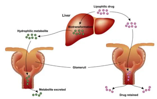
Fig. 6 shows the typical path of metabolism and excretion of a drug.
Figure 6 - Typical metabolic pathway of a lipophilic drug inside the human body. The drug is first metabolized by the liver and then it reaches the kidneys where it is eliminated. Taken from Merck Manual, 1982.
Introduction
41
1.2.2 Pharmacodynamics
Pharmacodynamics studies how drugs affect the human body and allows describing the receptor binding, the post-receptor effects, and the chemical interactions between drugs and receptors.
The pharmacodynamics of a drug can be affected by differences in the body mass, the gender or the race, physiologic changes due to disorders (e.g., genetic mutations, malnutrition, Parkinson disease, and diabetes), aging, or the interaction with other drugs. In particular, aging can alter the receptor binding or the post-receptor response sensitivity, while the interaction among drugs results in competition for receptor binding sites and/or alteration of the post-receptor response.
In our opinion, it is worth lingering briefly on the mechanisms of action of drugs and the role of receptors in those mechanisms.
In fact, drugs have to interact with receptors in order to act effectively. Receptors are macromolecules involved in chemical signaling between and within cells and can be located on the cell membrane or inside the cytoplasm. The activated receptors will then directly or indirectly regulate cellular biochemical processes.
In general, the molecules that bind a receptor are called ligands and can activate or inhibit a receptor. Each ligand can interact with multiple receptor subtypes and bind to particular regions of a receptor called “recognition sites”. The interaction between the ligand and the receptor is influenced by external factors as well as by intracellular regulatory mechanisms, for instance the density of receptors.
Receptors are selective and this selectivity represents the degree to which a drug acts on a given site respect to other sites. The degree of interaction between the molecule of a drug and the receptor depends on the probability that the molecule occupies a receptor at any instant and on the intrinsic efficacy that represents the degree to which a ligand activates a receptor and leads to the cellular response. These characteristics mainly depend on the chemical structure of the drug. Fig. 7 shows a simple schematization of the interaction between the drug and its receptor.
Figure 7 - Interaction between a drug and its specific receptor. The pharmacological effect is explicated through this interaction. Taken from Merck Manual, 1982.