Scuola Normale Superiore
CLASSE DI SCIENZE
P
H
D
T
HESIS IN
N
EUROSCIENCE
From in vitro evolution to
protein structure
Candidate:
Marco Fantini
Supervisors:
Annalisa Pastore
Antonino Cattaneo
ABSTRACT
In the nanoscale, the machinery of life is mainly composed by macromolecules and macromolecular complexes that through their shapes create a network of interconnected mechanisms of biological processes. The relationship between shape and function of a biological molecule is the foundation of structural biology, that aims at studying the structure of a protein or a macromolecular complex to unveil the molecular mechanism through which it exerts its function. What about the reverse: is it possible by exploiting the function for which a protein was naturally selected to deduce the protein structure? To this aim we developed a method, called CAMELS (Coupling Analysis by Molecular Evolution Library Sequencing), able to obtain the structural features of a protein from an artificial selection based on that protein function. With CAMELS we tried to reconstruct the TEM-1 beta lactamase fold exclusively by generating and sequencing large libraries of mutational variants. Theoretically with this method it is possible to reconstruct the structure of a protein regardless of the species of origin or the phylogenetical time of emergence when a functional phenotypic selection of a protein is available. CAMELS allows us to obtain protein structures without needing to purify the protein beforehand.
Table of contents
ABSTRACT 1 Table of contents 2 1 Introduction 5 1.1 Evolutionary Couplings 6 1.1.1 Mutual Information 71.1.2 Direct Coupling Analysis 10
1.1.3 Fitness Landscape 12
1.2 Molecular Evolutions and Mutagenesis 13
1.2.1 The political events, war, and the chance proximity of key individual behind the
discovery of mustard gas mutagenesis 13
1.2.2 Error prone polymerase chain reaction 16
1.2.3 Mutagenic nucleotide analogs for random mutagenesis 17
1.2.4 In vivo continuous evolution 19
1.2.5 Deep mutational scanning 21
1.2.6 An artificial selection 22
1.3 Sequencing 24
1.3.1 Traditional sequencing before high-throughput parallelization 24
1.3.2 The massive parallel sequencing revolution 26
1.3.3 The next “next generation”: 3rd generation NGS 27
1.3.4 Nanopore Technologies 28
1.3.5 Pacific bioscience SMRT technology 29
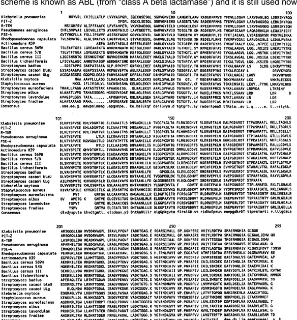
1.4 TEM beta lactamase 32
1.4.1 History, nomenclature and numbering of beta lactamase 32
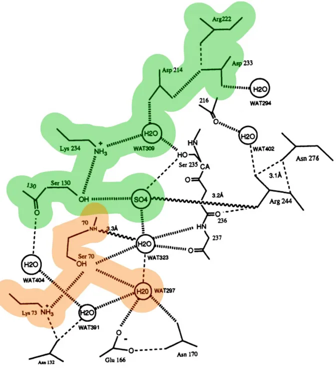
1.4.2 Mechanism of antibiotic resistance 36
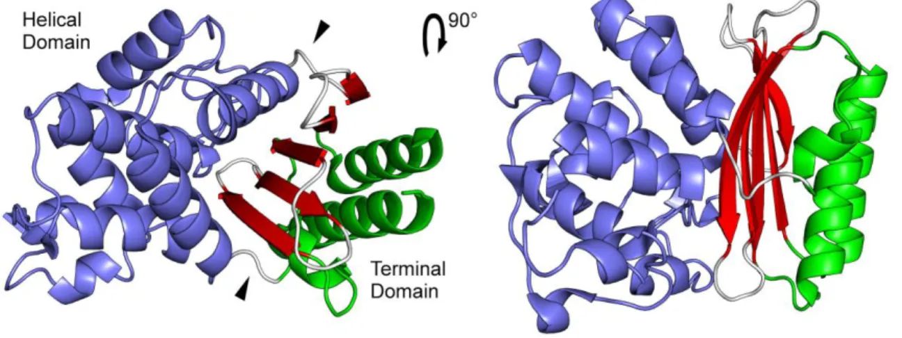
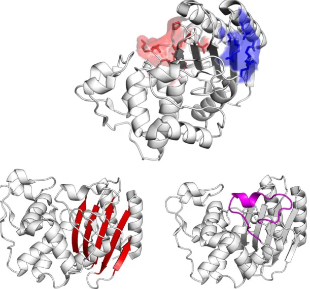
1.4.3 TEM-1 β-lactamase structure 38
1.4.4 A gold standard for molecular evolution 42
2 Results 43
2.2 Mutagenesis 47
2.2.1 Plasmid creation and primer design 47
2.2.2 Mutation strategy 49
2.2.3 Mutagenic nucleotide analogs 49
2.2.4 Error prone PCR 51
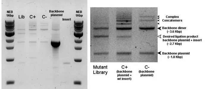
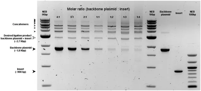
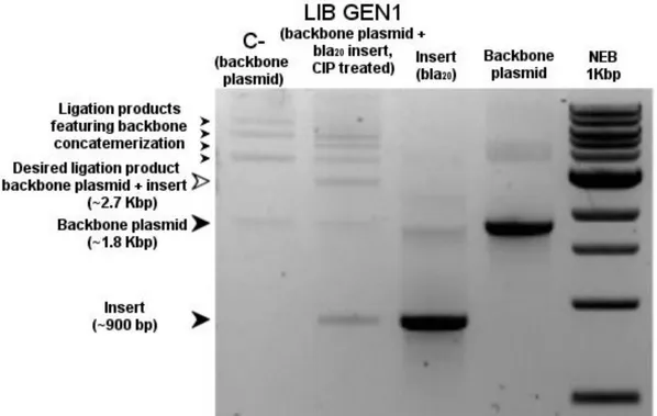
2.2.5 Ligation strategy optimization 54
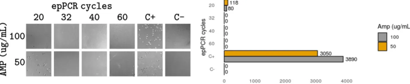
2.2.6 Library transformation and antibiotic concentration 59
2.2.7 Selection media 61
2.3 Molecular Evolution 64
2.3.1 First generation of molecular evolution (GEN1) 64
2.3.3 Direct coupling Analysis (GEN1) 76
2.3.4 Fifth generation of molecular evolution (GEN5) 80
2.3.5 Direct coupling Analysis (GEN5) 85
2.3.6 Twelfth generation of molecular evolution (GEN12) 92
2.4 Molecular evolution in DCA 103
2.4.1 Molecular evolution libraries meet the expected quality and mimic natural
variability. 103
2.4.2 The mutational landscape of the evolved library reflects the structural features of
TEM beta lactamases 108
2.4.3 The predominant Direct Coupling Analysis predictions are short range interactions
where the co-evolution effect is stronger 114
2.4.4 Improving the prediction power in key areas and retrieval of long range interactions 115
3 Discussion 120
4 Materials and methods 124
4.1 Plasmid construction & cloning 124
4.2 Error prone PCR 124
4.3 Library construction 125
4.4 Selection 125
4.5 Sequencing 125
4.6 Direct Coupling Analysis 126
4.7 Partial Correlation 127
4.8 Other bioinformatic tools 127
Note:
Most of the experiments and results featured in this thesis were published on October 2019 on the journal “Molecular Biology and Evolution” (MBE) (Fantini et al., 2019) and some parts of this thesis are taken verbatim from the article. The datasets used in this study are publicly available with the SRA accession codes SRX5562455, SRX5562456 and SRX5562457 or with the BioProject accession code PRJNA528665
1 Introduction
Shape and function are linked. In our everyday life most of the physical objects we come in contact with are shaped in a way that allows them to exert a certain function on the
surroundings. This is applicable to both manmade objects, like needles or gloves, and naturally selected creations, like thorns. This happens because shape is one of the most immediate ways to achieve a task, and it is used at the end of a designed process or naturally as a convenient way to gain an advantage under selective pressure.
Nature provides several examples of the adaptive characteristics connected to a particular shape, like wings or thorns. Even if bird and bat wings derive from different anatomical structures, they share the same shape because the trait is associated with the ability to fly. Identically for thorns: a rose prickle derives from shoots while a cactus spine was originally a leaf. Both evolved because the pointy shape acts as a deterrent for herbivores.
Inside the cell, the shape of proteins and other macromolecules is the most important attribute that allows them to exert the biological processes that form the machinery of life. Various organisms carry slightly different variations of the same proteins, but those protein variants will inevitably assume similar structures to express their intended function.
Everyday structural biologists use several techniques, like cryo-EM, crystallography or NMR, to reconstruct the structure of proteins. Studying the structure is what makes it possible to
understand the functional details and the mechanism of action of the proteins.
I wondered if it were possible to do the reverse: to get the structure by analysing the variants that express the function.
Aim of the Thesis
The aim of this thesis' project is to prove that the variability obtained by in vitro evolution is sufficient to support the reconstruction of a protein structure or to identify some structural details of the protein.
I employed direct coupling analysis to infer the structural information and error prone PCR to generate the variability in vitro. TEM lactamase was chosen as model for the proof of
principle since it is considered the gold standard reference for directed evolution studies and confer the host bacterium a very easy to screen antibiotic resistance. A limiting key aspect of the method is the collection of digital information from the biological library. I overcame this obstacle by using a third-generation sequencing platform that was able to produce reliable results that could be fed to the bioinformatic pipeline.
1.1 Evolutionary Couplings
Life is a complex phenomenon based on a precarious equilibrium of molecular transformations in a cellular environment mediated principally by proteins and their interactions. Proteins are encoded in a simple alphabet of only a few “letters”, but when combined in words, i.e. the peptide chain, they can express a variety of different functions that encompass signalling, transport and enzymatic catalysis. The function of a protein is an ability conferred by its shape, which in turn is dependent on the specific sequence and the sequence of the amino acids that form the peptide chain itself. It happens that sometimes the genetic information of an organism is corrupted by some mutations and that is reflected in small differences in the peptidic chains of some proteins. An alteration of the sequence of these proteins might affect their shape and in turn this will be reflected in an alteration of their function. If these proteins are important for the survival of the host organism and the modification generates a protein shape which damages the function of the protein, the host will likely die or have a serious disadvantage over its peers. For this reason, these types of mutations are unlikely to persist for more than a few generations and are probably lost during the course of evolution. This is why we can easily identify the same protein in different species, as the proteins are not allowed to variate indiscriminately but the function restricts the type of variants there might exist. Moreover proteins, depending on their functions are more or less able to variate, especially in their critical residues, and this
information can be used in phylogenetic studies. Nevertheless, variation is very important, since it allows a greater chance to adapt to sudden changes of the environment. If we have a
population with a single form of a given protein and this particular form is not able to function in the new environment, the population will go extinct. A population with more variants of the protein instead has a higher chance that one of these forms is able to function in the new environment and thus this allows part of the population to survive. Life is based on a regulated balance between mutations and adaptation that fuel a transforming driving force of cellular beings we call evolution.
Now let’s consider the case of a single deleterious mutation in a protein which happens at the same time of a second mutation in a spatially close part of the same protein. There is a chance that this second mutation can compensate the deleterious effect of the first. A charged residue can be compensated with an opposite charged one or a net loss of charge can be compensated with new charged residues appearing in the same area. Steric hindrance is the same, a new bulky residue can be accommodated if a spatially close one becomes smaller and vice versa. This co-occurring compensating mutations does not change nor the shape nor the function of the protein significantly and thus became part of novel variants of the protein that can persist during evolution. The key aspect of this phenomenon is that these joint mutation events leave an easy-to-spot trace in the evolution we can use to reconstruct which parts of the peptidic chain are close to each other. If a sufficient number of these are collected it is even possible to reconstruct the structure of the protein itself.
In a more technical explanation, when a set of variants of the same protein is retrieved it is possible to observe several positions that happen to mutate simultaneously during evolution. These positions are mutationally linked, since the single mutation might be harmful but the other one is able to compensate the former deleterious effect. They are thus “evolutionary coupled”, hence the name “evolutionary couplings”, and their co-occurrence analysed in a covariance
analysis is indicative of the spatial closeness in the structure of the protein of the amino acid positions that were altered by the mutations.
1.1.1 Mutual Information
The first attempts to rely on covariation to retrieve structural information belongs to the 80’s and 90’s (Altschuh et al., 1987; Göbel et al., 1994; Pazos et al., 1997) but the serious advancement in this field came with the advent of cheap genomic information in the sequencing era.
The earliest evolutionary couplings were calculated using Mutual Information (MI), a correlation estimator between variables that is not limited to numeric variables. Mutual Information as the name implies is a measure of the amount of information of a variable it is possible to capture from another.
Mutual information is a staple concept in information theory and I will only give a brief
introduction of the topic. For further information, I encourage the reader to look for a book on the subject like “Elements of Information Theory” of Thomas M. Cover and Joy A. Thomas (Cover & Thomas, 1991).
While the concept of information is very abstract, for discrete variables information is commonly approximated with the entropy of the variable of interest. Mutual information can be considered an extension of this interpretation of the entropy: while entropy reports the information of a single variable, mutual information describes the amount of information one random variable contains about another. The entropy of a variable X is a function of the distribution p of the variable. In formula, the entropy H of the variable x (x ∈ X) is defined by:
We can extend the concept to two or more variables. if we have two variables, X and Y, with a given distribution p, their joint entropy H is defined by:
Since 0 ≤ p ≤ 1, log(p) is always negative and thus H is always positive.
We can also define the conditional entropy of a random variable given another as the expected value of the entropies of the conditional distributions, averaged over the conditioning variable.
The entropy of two variables, their jointed entropy and their conditional entropies are closely linked since the entropy of two variables is the entropy of one plus the conditional entropy of the
other:
which is very easy to demonstrate:
Another important estimator is the relative entropy, which is a measure of the distance between two distributions. Mutual information is the distance of the joint probability distribution p(x,y) from the product distribution p(x)p(y). In formula:
where X and Y are two random variables with a joint probability function p(x, y) and marginal probability functions p(x) and p(y).
We can now observe an interesting relationship between mutual information and the entropies of the variables since:
Thus, mutual information is a measure of the information that one variable contains about another one. Numerically it equals to the reduction in the uncertainty of one random variable due to the knowledge of the other.
The relationship between H(X), H(Y), H(X, Y), H(X I Y), H(Y I X) and I(X, Y) can be represented in a Venn diagram where the mutual information corresponds to the intersection of the
information in X with the information in Y (Figure 1.1.1).
Figure 1.1.1 Venn diagram representing the relationship between the entropies.
In layman terms, we can comprehend these estimators using the weather as an example. We can have information about the weather in Rome and the weather in Milan. The weather in Rome give us also a little bit of information about the weather in Milan, because Rome and Milan are geographically close. This small amount of information is the mutual information. On the other hand, when the variables are more or less independent, like the weather in Rome and the weather in Beijing, the amount of information one can obtain from the other is close to zero. This analogy also holds for the residues of a protein. When the fold of the protein puts two residues close to each other, their entropies can capture this spatial closeness with a non-zero mutual information. On the other hand, residue spatially distant are less likely to have a
conspicuous mutual information. Reversing this paradigm, it is possible to infer the spatial closeness of two residues in a folded protein by looking at the mutual information of its residues.
1.1.2 Direct Coupling Analysis
The traditional correlation-based algorithms used for this analysis were effective but rather crude and suffered a lot of the confounding effects generated by indirect correlations. Let’s take, for example, a small network where amino acid A is linked to amino acid B and amino acid B is linked to amino acid C. In this network A and C indirectly covariate since they both respond to alterations of B, even if they might be far away in the protein structure. Another example might be a substitution in a faraway position of a protein that caused a conformational change in the protein that affect the interaction between other residues of the same protein. These residues are all correlated even if they lack a direct physical interaction.
The mutual information approach is defined local, since only a single residue pair is considered at a time. To overcome the problem, we require a global statistical model, where all the pairs are appraised simultaneously.
A sequence “A”, aligned to the other members of the protein family, is defined as a vector A = (A1, A2, A3, …, AN) where Ai represents the amino acid of the sequence at position i of the
acids and a symbol for gapped regions. The simplest global model P for a maximum likelihood approach is a function of A, minimizing the number of parameters we have to determine:
Model parameters are the couplings eij(Ai, Aj) between amino acid Ai in position i and amino acid
Aj in position j, and local biases hi(Ai) describing the preference for amino acid Ai at position i.
Z is the partition function:
and is used for the normalization of P.
Obtaining the best fitting model for the coupling eij is a computational hard task and usually
researchers use different approximation to simplify the task (Balakrishnan et al., 2011).
Once the eij and hi parameters are retrieved, the direct information is calculated from the model.
Direct information allows to disentangle the correlation network of the systems, favouring the identification of the strongest interactions to suppress the indirect correlations.
In an elegant way this was shown in a cardinal paper of Marks and colleagues (Marks et al., 2011) where both mutual and direct information were put in comparison in a self-explanatory graphical form (Figure 1.1.2).
Figure 1.1.2 (from (Marks et al., 2011)) Progress in contact prediction using the maximum entropy method. Extraction of evolutionary information about residue coupling and predicted
contacts from multiple sequence alignments works much better using the global statistical model (right, Direct Information, DI) than the local statistical model (left, Mutual Information, MI). Predicted contacts for DI (red lines connecting the residues predicted to be coupled from
sequence information) are better positioned in the experimentally observed structure (grey ribbon diagram), than those for MI (left, blue lines), shown here for the RAS protein (right) and ELAV4 protein (left). The DI residue pairs are also more evenly distributed along the chain and overlap more accurately with the contacts in the observed structure (red stars [predicted], grey circles [observed] in contact map; centre, upper right triangle) than those using MI (blue [predicted], grey circles [observed]; centre, lower left triangle).
1.1.3 Fitness Landscape
Direct correlation analysis is not the only technique that is used to infer evolutionary couplings. In particular, in mutational studies emerged the strategy of analysing the protein mutational landscape by looking at the fitness of the variants in selective conditions.
In general, the fitness landscape of a protein describes how a set of mutations affect the function of a protein of interest (Hartman & Tullman-Ercek, 2019). The function of a protein is typically evaluated indirectly performing a phenotypic assay, usually by testing the growth of the
host organism under selective pressure but also, more recently, with some protein-dependent fluorometric/colorimetric assays. To quantify the advantage or disadvantage the mutations confer to a protein, a deep sequencing of a mutagenized library of variants of the target protein is performed, collecting samples of variants before and after the exposure to the selecting environment.
The selective pressure will increase the frequency of mutations that confer a functional
advantage while deleterious mutations will decrease in frequency. The fitness is defined as the logarithm of the ratio of the frequencies before and after the selection of a given mutant, normalized to the ratio of the frequencies of the wild type variant in the same samples. When two or more mutations are independent, the fitness of the multiple-mutations variant is equal to the sum of the fitness of the single variants. In a paradigm where the fitness of a protein is determined by the overall function of the protein, like in a screening for the ability to grow in a selective media, it is possible to determine the evolutionary couplings by looking at the
differences between the single mutant fitness and the combined mutant fitness. In general, by subtracting from the fitness of a double mutation the fitness of the single constituting mutations, one can infer if the interaction between these mutations is positively affecting the function of the protein or vice versa. A complete fitness landscape that analyses every possible variant of a protein is often used to study evolution, to identify proteins with new and useful properties, or to quantify mutability. The main difference between a fitness landscape and an evolutionary landscape is that the former tries to operate outside the paradigm of evolution, allowing the identification of characteristics of the protein that the constraints of a progressive evolution might have precluded.
1.2 Molecular Evolutions and
Mutagenesis
Molecular evolution is the course of modifications of the sequence that constitute a biological molecule in succeeding generations.
In this manuscript however, I will use molecular evolution to indicate the in vitro molecular evolution a smaller umbrella term that includes a wide variety of techniques that perform in vitro mutagenesis of a cloned gene coupled with powerful screening methods to select functional variants of the protein it codes. Molecular evolution is especially useful to understand the role of functionally significant positions of a protein when the molecular mechanisms that regulate the function in not entirely understood. Molecular evolution is associated to a series of topics and analyses that relate to the impact of mutations in the population, to the development of new genes or new functions or to study evolutionary driving forces.
Historically the driving forces for molecular evolution mutagenesis were of physical nature, e.g. ultraviolet light or ionizing radiation induced DNA damage, or chemical nature, employing mutagens like mustard gas.
Nowadays, the most common methods to introduce random mutation in a sequence are chemical mutagenesis (Shortle & Botstein, 1983), alteration by mutation-inducing bacterial strains (Husimi, 1989; Toprak et al., 2012), incorporation of mutagenic nucleotide analogues (Zaccolo & Gherardi, 1999), DNA shuffling (Stemmer, 1994), incorporation of randomized synthetic oligonucleotides (Wells et al., 1985) and generation of mutations during the copy of the nucleic sequence by a low fidelity polymerase (Cadwell & Joyce, 1992).
1.2.1 The political events, war, and the chance proximity of key individual
behind the discovery of mustard gas mutagenesis
Before delving into the serious part of the thesis, allow me to digress and tell the curious story that defined the history of mutagenesis, a tale that greatly inspired me during some difficult periods of my PhD internship. After all, it is impossible to discuss the origin of mutagenesis without narrating the extraordinary events and circumstances that revolved around the discovery of the first chemical mutagens: the mustard gas. This chapter will recount the story around the discovery of Charlotte Auerbach and John Michael Rabinovich, later known as Robson, as it is portrayed by the anecdotal report of the historical testimonies collected by Geoffrey Beale (Beale, 1993).
In 1940 the notion of gene as a unit of heredity was well established but the work of Griffith and Avery on the nucleic acid nature of the genetic information was still largely unknown.
One of the known properties of the gene was the ability to mutate, at the time defined as the transition from one an allelic form to another. Hermann Joseph Muller, future Nobel laureate for his work on the effects of radiation, demonstrated that mutation could occur both as a natural process or as a result of exposure to ultraviolet light or ionizing radiation such as X-ray. It was thought that X-ray induced mutation could be used to investigate the nature of the genes but soon it was evident that the type of mutations induced by radiation was not suited for such a
study and Muller itself hoped that a mutagenesis induced by chemicals could yield better information. For this reason, the discovery of chemical mutagenesis by Auerbach and Robson, in collaboration with Muller was treated as a sensational breakthrough in the history of genetics. The key figure of this tale is Charlotte “Lotte” Auerbach, a scientist that was born in 1899 to a Jewish family in Krefeld, Germany. She was schooled in Berlin and attended lectures in the university of Berlin, Würzburg and Freiburg. At the age of 25 she started working under Otto August Mangold in Berlin-Dahlem. This situation was not congenial since Mangold, being a Nazi, was constantly antagonizing her for her Jewish origin. On one occasion discussing a change in her project, Mangold replied to a concern she raised saying: “Sie sind meine
Doktorantin. Sie müssen machen was ich sage. Was Sie denken hat nichts damit zu tun.” that
translate to "You are my doctoral student. You have to do what I say. What you think has
nothing to do with it.". After Hitler was elected chancellor in 1933, Charlotte decided to leave the
country to move to Britain with the help of an Anglo-German close family friend, chemistry professor Herbert Max Finlay Freundlich. She was shortly introduced to Francis Albert Eley Crew, head of the Institute of Animal Genetics at Edinburgh, who offered her a very modest position at his institute. Despite her financial situation was precarious, the intellectual
atmosphere in the laboratory was very lively and with the help of her colleagues Lotte taught herself some genetics. The Institute was at the time one of the few places in Britain where genetic research was carried out and Crew himself collected a group of what Auerbach called “waif and strays” on minimal salaries from continental Europe (among them Peo Charles Koller, Guido Pontecorvo, Rowena Lamy, Bronislaw Marcel Slizynski, Helena Slizynska and Hermann Joseph Muller).
In 1939, with Crew’s help Charlotte was able to obtain the British nationality preventing the incarceration as an enemy alien following Britain’s declaration of war on Germany. At the time there was a paranoid spy fever in Britain, and it was expected that German parachutists would invade from the sky. On one occasion she was reported to the police because a mysterious tapping noise (her typewriter) was heard from her apartment, “from a room occupied by a lady with a strong German accent”. In 1940, when Italy entered the war, Guido Pontecorvo, a colleague and friend of hers, was unable to avoid the confinement as an enemy alien and was incarcerated in an internment camp on the Isle of Man.
In 1938, Crew peremptorily announced to her that she was to work with Muller. Muller suggested her to work with several known carcinogens to obtain chemical mutations in
Drosophila, however they all failed to produce the expected results. Following these attempts, she stated to work on mustard gas as a collaboration with Robson and Alfred Joseph Clark. Experimentation on mustard gas originated from the observation by Clark of the similarities between radiation damage and the effect of mustard gas, especially in regard to eye injuries. Clark got the idea that these long-lasting effects might act on the genetic materials in cell nuclei. At the outbreak of the second world war it was expected that chemical warfare would be used in the coming battle, as it had been in the war of 1914-18, so much that soldiers were given gas masks in cardboard boxes to carry around wherever they went. Clark had a research contract with the government to research the effect of mustard gas, especially in eyes injuries.
Due to the strategic importance of the research for the war, the Muller team was forbidden to use the word “mustard gas” in any communication as it would have contravened the secrecy rules imposed by the government. In everyday communication, “substance H” was the term
used. Of course, since it was impossible to publish any results, there was very little interest on the subject.
The first experiments begun in November 1941 and were done on the roof of the pharmacology department in Edinburgh. Liquid mustard gas was heated in an open vessel and flies were exposed to the gas in a large chamber. All people involved quickly started to develop serious burn on their hand. Lotte was warned by her dermatology not to expose her hands to the gas again or she could develop serious injuries while Robson started wearing gloves. With the crude apparatus they employed it was impossible to control the amount of mustard gas to which the flies were exposed, and results were hard to replicate. After gas treatment the surviving flies were analysed by Muller ClB method, trying to identify X-linked mutations.
This tale would be incomplete without clarifying the struggle and the emotional distress that Lotte was facing during this period. In 1942 she wrote to Muller, her supervisor, who had moved to Amherst College in America:
“Dear Dr. Muller, I am afraid you will be disappointed how little further I have progressed with my work since I last wrote. It was not however my fault through laziness, but terrible difficulties with the dosage. From May to December I have done one experiment after the other without being able to reproduce the right dosage again . . . Robson insisted on a repetition of the original experiment for sex-linked lethals. As I expected, the result when it at last came off was completely confirmatory: 68 lethals and four semi-lethals in 790 tested chromosomes. In addition there were some visible mutations among the semi-lethals . . . .
Yours very sincerely, Lotte Auerbach”
However, Muller did not reply to Lotte’s letter or perhaps his reply was sunk crossing the Atlantic Ocean so Lotte wrote again:
“Dear Dr. Muller, . . . I hope you won’t think me ungrateful if I admit that in spite of my pleasure I was disappointed that there was no word from you or Thea [Muller’s wife] . . . It is such a long time since we last heard from you, and I often wonder how life is treating you two just now. I hope, very kindly. In any case, here are my sincerest wishes that it will do so in 1943. I also was hoping for a word from you on my work. I am getting rather discouraged by the lack of interest I encounter everywhere. And the fact that you don’t write about it makes me suspect that I have disappointed you very much by my various reports . . . All the same-hearty thanks once more, and the kindest regards for Thea and you.
Yours, Lotte A.”
Luckily for everyone this tale does have a happy ending. In March 1942 the first experiment report was sent to the Ministry of Supply in London. In this first report Robson and Lotte
reported the generation of sex-linked lethal mutations generated by treatment with substance H (mustard gas), as well as breaks and rearrangements of chromosomes. In a later report they mention a difference in the susceptibility to mustard gas of different drosophila strains. The third report showed that the mustard gas acted directly on chromosomes rather than exerting an effect on cytoplasm. The fourth report was focused on the induction of visible mutations by mustard gas, the differences between X-ray damage and chemical damage and a draft of the possible genetic action of the gas. After the war, at the Eighth International Congress of Genetics in Stockholm in 1948, Lotte delivered a comprehensive review entitled “Chemical Induction of Mutations.” and was applauded by Muller, who was then the president, which gave Lotte enormous satisfaction. In 1948, she was awarded the Keith Prize of the Royal Society of Edinburgh. After receiving her D.Sc. degree in 1947, Lotte was appointed Lecturer in the Institute of Animal Genetics. From 1959 to 1969 she served as Honorary Director of the Unit of Mutagenesis Research which the Medical Research Council had established at Edinburgh. Finally, after her retirement in 1969, she was made a Professor Emerita.
At the end of his anecdotal report on Charlotte’s life and discovery Beale wrote his personal interpretation of the whole situation explaining to everyone the moral of this story:
“No doubt many factors contributed to the proposal (and successful prosecution) of the work. Among these we may mention: (1) the imminence of World War II, leading to the support for Clark’s work on mustard gas in Edinburgh; (2) the presence in Edinburgh at the same time of Clark, Robson, Lotte, and above all Muller, who met frequently for discussion of research; and (3) the existence of Crew’s Institute of Animal Genetics, at which there was a lively group creating an atmosphere favorable for scientific work. Lotte herself informed me that, speaking ironically, even Hitler could be held to some degree responsible, as he had forced her to leave Germany and abandon school teaching for scientific research. But there seems no doubt that it was the expertise in Drosophila research methods and perseverance of Lotte along with the intrepid, perhaps foolhardy handling of the chemical that were mainly responsible for the success of the work”
1.2.2 Error prone polymerase chain reaction
Error prone PCR is a highly versatile mutagenesis technique that rely on the inaccurate copying by a DNA polymerase in a PCR reaction to produce a collection of mutated sequences. Error prone PCR is one of the oldest and most used strategies in mutagenesis thanks to the simplicity of the technique and the fact that most mutagenesis experiments are aimed to identify a small number of mutations that increase the stability or activity of the target protein. The error
propensity that gives its name to the technique is generated and enhanced by a series of factors that alter the fidelity of the polymerase during in vitro DNA synthesis. In its original formulation (Cadwell & Joyce, 1992; Leung, 1989) the fidelity of the PCR was reduced by increasing the concentration of MgCl2, adding MnCI2, using an unbalanced
ratio of nucleotides (an increased 1 mM concentration of dGTP, dCTP, and dTTP together with standard 0.2 mM concentration of dATP), increasing the concentration of the polymerase, and increasing the extension time. Under these conditions the reported rate of mutagenesis per position could go as high as 2%. Cadwell and Joyce (Cadwell & Joyce, 1992) however argued
that in the setup proposed by Leung et al., the mutated sequences obtained after mutagenesis display a strong A→G and T→C transition bias that steered the DNA toward a high GC content. The nucleotide concentration unbalance Leung used in his work was drawn from a previous study which demonstrated that in their very simple model the mutation rate could only be increased by lowering the concentration of dATP relative to that of the other three dNTPs. Lowering the concentration of one of the other three nucleotides produced little effect on the mutation rate (Sinha & Haimes, 1981). The lack of deoxyadenosine as a substrate promoted several non-Watson-Crick base mispairs, in particular G-T mispairs, and this condition leads to an excess of A→G and T→C transitions on the final product. To correct this issue, Cadwell and Joyce tested several imbalanced ratios of deoxynucleotide and were able to identify a condition in which the frequencies of AT→GC and GC→AT mutations became identical, albeit producing a lower final yield of 0.6% mutations per nucleotide position. It is important to notice that even if this new protocol produced a balanced ratio of 𝐴𝑇→𝐺𝐶
𝐺𝐶→𝐴𝑇mutations, there is still a significant preference for T→X changes (X ≠ T) and X→A changes (X ≠ A) and the observed 0.75:1 transitions to transversions ratio is different to the unbiased ratio of 0.5:1.
Several different types of polymerase have been tested to maximize the probability of a wrong base incorporation, among them the Klenow fragment (of E.coli polymerase I) (Keohavong & Thilly, 1989), T4 DNA polymerase (Sinha & Haimes, 1981), Sequenase (a modified T7 DNA polymerase) (Ling et al., 1991), Taq DNA polymerase (J. Chen et al., 1991; Eckert & Kunkel, 1990, 1991; Ennis et al., 1990; Tindall & Kunkel, 1988) and Vent (Thermococcus litoralis) DNA polymerase (Mattila et al., 1991).
In this group, the lowest fidelity is shown by the Taq polymerase, the one used by Cadwell and Joyce, with a “natural” mean error rate of 0.001-0.02% (Eckert & Kunkel, 1990, 1991) per nucleotide each time the polymerase travelled over the template DNA.
1.2.3 Mutagenic nucleotide analogs for random mutagenesis
An alternative strategy for PCR-based mutagenesis is employing mutagenic nucleotide analogs that promote nucleotide base mispairing during amplification. This strategy was pioneered by Zaccolo and Gherardi (Zaccolo et al., 1996) with the usage of triphosphates of mutagenic nucleosides as substrates for a PCR-based mutagenesis.
They identified four conditions that defined a good mutagenic nucleotide analog: the substrate should be stable under the conditions of PCR cycling, well incorporated, be of high mutagenic efficiency and be able to direct both transition and transversion point mutagenic changes when used in combination.
At the time, there were several base analogue mutagens whose 5' nucleoside triphosphates had been characterized (N4-hydroxy-2'-deoxycytidine (Müller et al., 1978),
2-aminopurine-2'-deoxyriboside (Grossberger & Clough, 1981), 5-bromo-2'-deoxyuridine (Mott et al., 1984), O6
-methyl-2'-deoxyguanosine (Eadie et al., 1984; Snow et al., 1984), N4-amino-2'-deoxycytidine
1984), N6-hydroxy-2'-deoxyadenosine (Abdul-Masih & Bessman, 1986),
5-hydroxy-2'-deoxycytidine and -uridine (Purmal et al., 1994)).
N4-hydroxy-2'-deoxycytidine and N4-methoxy-2'-deoxycytidine both display tautomeric constants
between 10 and 30 (Brown et al., 1968; Morozov et al., 1982) (a tautomeric constant around 1 is required to induce transition mutations effectively) and are able to form a pair with both A and G, however the base pairing via the imino tautomers is sterically hindered due to the syn
preference of the N4-substituents (Morozov et al., 1982; Shugar et al., 1976).
The nucleoside dP (6-(2-deoxy-β-d-ribofuranosyl)-3,4-dihydro-6H,8H-pyrimido[4,5-c][1,2]oxazin- 2-one) is an analogue of N4-methoxy-2'-deoxycytidine but, due to its bicyclic ring structure, is
restricted to the anti conformation and it is able to form stable base pairs with both A and G. In 1996 Zaccolo and Gherardi (Zaccolo et al., 1996) demonstrated that the nucleoside triphosphate of dP (dPTP) would be a good substrate for the polymerases in PCR reactions. However, dPTP is only able to promote nucleotide transition mutations, and by itself is unable to explore the whole panorama of possible mutations since it cannot mutate a purine into a
pyrimidine or vice versa.
There are very few nucleoside triphosphate analogues capable of transversion mutations (Pavlov et al., 1994; Purmal et al., 1994; Singer et al., 1986, 1989). Among them only 8-oxo-2'-deoxyguanosine triphosphate (8-oxodGTP), one of the major products of DNA oxidation generated during cellular oxidative stress, appears to be a substrate for DNA polymerases adequate for mutagenesis (Pavlov et al., 1994; Purmal et al., 1994).
8-oxodGTP assumes the anti conformation when paired with cytosine (Oda et al., 1991), while adopts the syn conformation with adenine (Kouchakdjian et al., 1991) therefore allowing A→C transversion mutations during DNA duplication (Cheng et al., 1992; Maki & Sekiguchi, 1992; Shibutani et al., 1991).
The mutations generated by these analogues are heavily biased towards a single mutation type. Of the transition mutations elicited by the presence of dPTP in the reaction, the vast majority are A→G (46.6%) and T→C (35.5%), while G→A (9.2%) and C→T (8%) are rather rare. A→G and T→C transitions are the result of the incorporation of dP instead of a T in either strand during DNA duplication followed by a mispairing of the incorporated dP with a G in the subsequent cycle. Incorporation of dP when paired to a G in either strand occur at a much lower frequency and thus produce the mutational bias.
8-oxodGTP is more biased than dP and virtually generates only a single type of transversion mutations: A→C (38.8%) and the complementary T→G (59%). These transversions are the result of the incorporation of 8-oxodGTP instead of a T in either strand during DNA duplication. The frequency of the reverse C→A transversions is 40 times lower than that of the A→C transversions (Cheng et al., 1992).
Random mutagenesis of DNA using nucleotide analogues relies on a PCR reaction carried out with both dPTP and 8-oxodGTP. The two analogues are efficiently incorporated into DNA in vitro by Taq polymerase and this allows for point mutations to be introduced with high efficiency
into the target sequence by PCR. The mutational load of the final product can be regulated by limiting or increasing the PCR cycles performed in mutagenic condition.
Clones mutagenized with the combination of dPTP and 8-oxodGTP in standard mutagenic conditions can reach a mutation frequency of 1 × 10⁻³ per nucleotide.
1.2.4 In vivo continuous evolution
Continuous Evolution is a different approach to molecular evolution, limiting the handling steps of the operators to a bare minimum and aimed to generate to a self-sufficient and fast paced evolution system.
Badran (Badran & Liu, 2015) simplifies the requirement for Darwinian evolution to four fundamental processes: translation (that is not simply the biological concept of the RNA producing process but more in general when the evolving molecule is not identical to the information carrier), selection, replication, and mutation. Traditional molecular evolution methods handle each of these processes separately while continuous evolution systems integrate all of these into an uninterrupted cycle.
The first formulation of the technology dates back to the sixties with the hallmark publication of Mills, Peterson and Spiegelman (Mills et al., 1967) where they proved the possibility to evolve a minimal Qβ bacteriophage genomic RNA in an enriched in vitro system. The authors raised the interesting question:
"What will happen to the RNA molecules if the only demand made on them is the Biblical injunction, multiply, with the biological proviso that they do so as rapidly as possible?"
The authors provided an environment with plenty of nutrients and the replication apparatus and liberated the genome from the cellular confinement and the requirement of producing an infection machinery. The experiment was carried out as a set of serial reactions and as the experiment progressed, the genome multiplication rate increased and the product became smaller. By the 74th transfer, 83% of the original genome had been eliminated and the new genome was able to replicate up to 15 times faster. This new genome however could no longer direct the synthesis of new viral particles since this requirement was not implicit in the selection and many important genes were lost.
Additional studies, altering the tube environment and limiting different resources, extended this method to generate a continuous evolution of an RNA-mediated catalytic function (Wright, 1997), new promoters (Breaker et al., 1994), or other RNA related elements or function. These early methods were exclusively carried out in vitro where the parameters involved were easy to control but on the other hand they gave up the ability to study the untapped complexity of a cellular system and set aside the biological results of an in vivo selection method could produce.
The earliest alternatives to in vitro methods came with the introduction of chemostats and auxostats, culture vessel automations where the bacterial growth is maintained through the continuous regulated inflow of fresh growth medium. These platforms were particularly suited to support a directed bacteriophage evolution by maintaining a fresh pool of bacteriophage
mutation rates and are simple to collect and analyse, making them adequate model organisms for the initial in vivo directed evolution of selectable traits (Husimi, 1989).
One of the first studies that pioneered this method was the viral continuous evolution of the bacteriophage ΦX174 in E. coli and S. typhimurium to adapt to a high temperature environment (Bull et al., 1997). In this study an average of 1–2 mutations per 24 hours (corresponding to 0.2–0.5% of the viral genome, and 0.003–0.005 mutations per generation per kilobase) was generated in the absence of any added mutagens. In an expansion of this work, ΦX174 phage was propagated for six months, ∼13,000 phage generations (Wichman et al., 2005), and proved the very long-term potential of application of the technology.
A novel adaptation of the bacteriophage mediated evolution is phage-assisted continuous evolution (PACE) (Esvelt et al., 2011). PACE exploits the coat protein pIII from the
bacteriophage M13 to mediate infection and phage propagation. The bacterial host carry this protein under a transcriptional circuit regulated by the selection process. When the selective pressure produces a functional variant of the molecule of interest, pIII is produced and the virulence of the bacteriophage is restored, allowing a robust phage propagation in continuous culture. Meanwhile phages lacking functional pIII have no ability to propagate and are rapidly lost under continuous culturing conditions. The continuous flow of this system coupled with the steady infection of fresh cells allows mutations to accumulate only within the phage genome while the genome of the bacterial population is preserved.
The increasing popularity of bacteriophage mediated evolution promoted the development of several bacterial culture vessel for a monitored continual prokaryotic growth and in turn
facilitated the study of continuous directed evolution of bacterial populations. Bacterial evolution compared to the phage assisted counterpart carry two main advantages, namely an even simpler system and a broader range of gene size (while viral fitness impedes the transfer of big genes).
Toprak (Toprak et al., 2012) used bacterial evolution to follow parallel populations of E. coli under differing antibiotic selection pressures using a morbidostat. This apparatus is a bacterial culture device in which the concentration of antibiotic is periodically adjusted to maintain a nearly constant selection pressure, i.e. it increases the antibiotic concentration to preserve the bacterial growth speed. The populations were subjected to an evolutionary pressure under the driving force of different antibiotics, and followed using whole-genome sequencing to collect the mutations that provoked antibiotic resistance.
In both bacteria and phagic evolution, some applications may require an extensive mutagenesis and the basal rate of bacterial mutagenesis might not be enough to provide access to necessary genetic changes on a practical timescale.
A popular method used to enhance the bacterial mutagenic propensity was introducing an orthogonal, low fidelity polymerase in the bacterial genome. A famous implementation of this idea uses a modified E. coli DNA polymerase I (Pol I) where the error rate is increased to
promote the mutagenesis of the target gene (Camps et al., 2003) while limiting the damage on the core genome of the cell.
1.2.5 Deep mutational scanning
If targeted mutagenesis examines a limited number of protein variants with a specific question in mind and other types of molecular evolution generate a limited pool of variants, deep mutational scanning (Fowler & Fields, 2014) is aimed to obtain an exhaustive collection of all possible mutants of a protein and verify their functional viability. As reference for the scale of this
process, the average human protein is ~350 amino acids in length and it can yield 7,000 single mutations and over 22 million double mutations (Brocchieri & Karlin, 2005). The idea under the technology is rather old, after all alanine scan (Cunningham & Wells, 1989), in which each position of a protein is sequentially mutated to alanine, can be considered a limited ancestral version of this technology. A complete systematic mutagenesis instead was developed only relatively recently because it had to overcome two big challenges that could only be resolved with modern day technology. The first challenge was the generation of all of these variants in an efficient process, while the second was to be test and sequence the variant in parallel without the need to handle the individual mutant. In particular, the big leap forward in this context came with the development of mass parallel sequencing and high-throughput technologies.
Traditionally the most used mutagenesis method was random mutagenesis. It generated a very big library of 105-1011 protein variants and then this library was screened for the selected
function bringing the diversity down to a small size so that it could be Sanger sequenced. It is evident that the limitation was not the original diversity but the requirement of a small pool of sequence for the sequencing. In the first formulation mutational scanning was just a technique that combined selection with high-throughput DNA sequencing. Because the sequenced variants were now several hundred times the number of variants obtained from traditional sequencing, a harsh selection pressure is not required anymore to collapse the size of the mutagenic library. A mild selection does not cause a drastic high pass filter on the function of the survivor protein and allows a bigger spectrum of variation. Moreover, instead of observing only a survival of the fittest, it was now possible to observe the variation in the mutant
frequencies, and this variation is linked to the function of each variant. All variants harbouring beneficial mutations would increase in frequency, variants harbouring nearly-neutral
substitutions would display little to no variation, whereas variants harbouring deleterious mutations would decrease in frequency.
To construct these libraries, several methods can be used (Fowler & Fields, 2014), but in practice the methods that became indissolubly tied with the deep mutational scans are oligonucleotide based directed mutagenesis methods like PFunkel (Firnberg & Ostermeier, 2012). Oligonucleotide directed mutagenesis allows a very efficient and fast construction of large libraries of singly mutated variants but has difficulties when used to construct libraries of multiply mutated variants. The double mutant space around the average-sized human protein can in theory be completely explored by systematic mutagenesis but since the number of possible sequences increases geometrically with the protein length, and the next generation
sequencing albeit able to cover a vast collection is still limited, the approach rapidly loses the power to be exhaustive.
Another advantage of oligonucleotide-based mutagenesis is being able to selectively restrict the number of positions to be mutagenized, e.g. mutagenizing only few residues in a substrate binding site or in the catalytic pocket. This strategy enables to reduce the overall diversity of the library and increase the read count and the accuracy of the critical residues for the study.
1.2.6 An artificial selection
Molecular evolution is a two-step pipeline where the first step involves generating the diversity, that is the phase when the variants are built, and then the second step is the selection process. If mutations are the driving force of the evolution, the selection poses the constraints that guarantee the protein function. While the mutations are generating random variability, the
laboratory selection oversees the new variants authorizing only the conformations that follow the natural blueprint we are exploiting. The selection is always carried out as an evaluation of the target protein function or characteristic, and, as a consequence, it cannot be a generic task like mutagenesis but has to be designed on a case by case basis for each intended target. The most common selection processes are aimed to verify the preservation of the activity of an enzyme or the ability to bind an interaction partner. For instance, we can verify the activity preservation of a metabolic enzyme by analysing the conversion speed of the metabolites the enzyme catalyses or it is possible to verify the interaction ability in binding assay like in phage display. Given the scale of molecular evolution experiments, cumbersome assays are difficult to implement and most of the times the preferred assays are the ones that permit a rapid and parallel screening for the intended function. Common assays are survival assay to test the activity of essential genes, binding assays to test the interaction capability of the target protein and assays that exploit the ability of the protein to convert some chromogenic substrate. Survival assays are the most straightforward type of assays, given that only the cells that carry a functional copy are allowed to survive. To have a rough approximation of the number of genes that can undergo this type of selection we can use the Venter list of essential genes for a
minimal genome. In its final formulation, the minimal Genome of Syn3.0 had 473 genes (438 protein and 35 RNA-coding genes) classified as essential, ~31% of which were not assigned to any specific biological function. Ironically, even if the selection of these is based on their
molecular function, it is not strictly necessary to understand the function of these genes, since the complex ability to survive is the actual phenotypic trait that is sieved for functionality. Gene essentiality is tightly linked to the cell type and to the environment. If the growth medium is devoid of tryptophan, the genes involved in the biosynthesis of tryptophan are essential, but for cells grown in a medium where the amino acid is available, these genes are not critical
anymore. Some other genes, notably antibiotic resistance genes, do the opposite: in a normal environment do not confer any selective advantage but become essential when the bacterial cell is exposed to the antibiotic. The ampicillin resistance gene TEM-1 beta lactamase, which
catalyses the hydrolysation of the β-lactam ring of many antibiotic penicillin derivatives and was the protein target of the mutagenesis done in this thesis, is part of this class of genes.
The other very common selection strategy in mutagenesis experiments is based on
molecules in solution. Notably, this group includes proteins involved in heteromeric complexes, protein involved in some functional transient interaction and receptor-ligand pairs. In order to select the protein variants where the interaction is still present, the protein is exposed to its interaction partner, often conjugated to some purification mechanism, and then purified by coprecipitation or retention exploiting the association to the interacting protein. Phage display and more in general most types of display technologies are the most popular selection platforms for functional interaction assays. They work by directly linking the genotype to the phenotype and are able to select for the functional interaction of the protein and at the same time collect the gene of these functional variants.
Selection can be either carried out in vitro (display technologies) or in vivo. Most of the
organisms used for in vivo screening procedures are characterized by a fast replication time and an easy transformation strategy. Common organisms used for selection are fast growing
bacteria, like Escherichia coli, or yeast, such as Saccharomyces cerevisiae. The main advantages of a bacterial selection system are the growth time and the transformation
efficiency, while the yeast models have a eukaryotic genetic background that is preferred when the aim is to study a eukaryotic protein and can make use of the eukaryotic cell
1.3 Sequencing
Molecular evolution creates the conditions to compel a given molecule to undergo an adaptive mutagenesis in order to survive the selective environment. If the desired output for the evolution is to obtain novel organisms that survive the selective pressure, then all the surviving cells achieve this purpose since each of them carry new functional variants of the molecule.
In other applications however the cell itself is not the desired output of the evolution but rather the desired information is the composition of the variant molecules that allowed the hosts to survive.
To obtain this information, sequencing the variant molecule is essential. Traditional experiments on synthetic evolution are focused on observing the mutational landscape of the protein of interest (K. Chen & Arnold, 1993; Esvelt et al., 2011) or study the trajectories of evolution. This was achieved by analysing the emergence of the patterns of mutations that appear
progressively during the course of an evolution experiment in one or more samples subjected to the same selective pressure (Hillis & Huelsenbeck, 1992; Zaccolo & Gherardi, 1999).
Sanger sequencing is used when relatively few variants are screened (Jacquier et al., 2013) or when the newest sequencing technologies were not yet available (Zaccolo & Gherardi, 1999). In recent applications next generation platforms are employed to increase the throughput of the output so that several thousand or million variants are recovered in a single sample analysis (Olson et al., 2014). Second generation sequencing platform are however heavily constrained on the length of the molecule and cannot be used on any protein of interest.
Our application requires the sequencing of library made of hundred thousand to a few million different elements in size where each of the reads must cover the whole molecule variant, thus neither Sanger sequencing or traditional next generation platforms are sufficient.
We pioneered the usage of single molecule third generation sequencing on library of gene variants evolved by molecular evolution to remove the size restriction to our data collection. The following sections will provide an introduction to both traditional and recent sequencing technologies to give the reader a complete panorama of the possible sequencing platforms that could be used to collect the data, discussing their advantages and drawbacks.
1.3.1 Traditional sequencing before high-throughput parallelization
The first attempt to create a widespread, easy and general sequencing technique began with the experimentation of Sanger and Coulson in 1974 (Sanger et al., 1974; Sanger & Coulson, 1975). The protocol involved partial DNA synthesis and a separation by electrophoresis through polyacrylamide gels to discriminate the polynucleotides lengths. The first step of the protocol is an initial asynchronous synthesis of the target DNA by polymerase I which extend the primer oligonucleotide and copy the template. This step generates a great number of oligonucleotides of different lengths, all starting from the primer. Afterwards, two second polymerisation
reactions are performed: a ‘plus’ reaction (from (Englund, 1971, 1972) ), in which only a single type of nucleotide is present, thus all extensions will end with that base, and a ‘minus’ reaction (from (Wu & Kaiser, 1968)), in which the other three nucleotides are used, which elongate the sequences up to the position before the next missing nucleotide. When all 4 ‘plus’ and 4 ‘minus’ reactions are completed and run on acrylamide gels, one can compare the patterns and deduce the sequence. For each position there should be a ‘plus’ band, corresponding to the nucleotide
in the position and a ‘minus’ band, corresponding to the next nucleotide in the chain. Deviations from this rule, showing differences in the ‘plus’ and ‘minus’ systems, allow the discrimination of adjacent identical nucleotides in the chain (Figure 1.3.1).
Also, in the mid-seventies Maxam and Gilbert (Maxam & Gilbert, 1977) developed a sequencing system based on chemical degradation at specific base types of the target sequence. This sequencing requires first to radiolabel the 5’ or 3’ end of the DNA fragment, then a chemical treatment partial digests the target sequence in the presence of specific nucleotide bases. There are several reactions that can target specific nucleotide or combinations, but commonly only four are used: purines (A+G) are depurinated using formic acid, guanines are methylated by dimethyl sulfate, cytosines are hydrolysed by hydrazine and sodium chloride, the pyrimidines (C+T) are hydrolysed using hydrazine without salt. The modified base promotes a site-specific cleavage when piperidine and heat are provided to the solution. The labelled fragments generated by the strand breaks are then migrated in an acrylamide gel and the sequence deduced by comparing the patterns of the four reactions (Figure 1.3.1).
Figure 1.3.1 Examples of the earliest traditional sequencing and sequence assignment.
The major breakthrough in sequencing technology, so much that the technique is still used nowadays, came in 1977 with Sanger’s chain-termination sequencing technique (Sanger et al., 1977).
The strategy exploits the incorporation in the nucleotide chain of the 2’3’-dideoxyribonucleotides (ddNTPs) version of the four nucleotides which prevents any further polymerization of the nascent chain in a DNA synthesis reaction.
A mixture of a radio labelled ddNTP and standard deoxynucleotides in a DNA extension reaction produces a collection of DNA strands of different lengths, all ending with the dideoxynucleotide which prevents a further extension of the chain.
Four different reactions, each involving a different dideoxynucleotide, generate a specific pattern when migrated in an acrylamide gel that can be used to infer the composition and sequence of the target nucleotide chain.
1.3.2 The massive parallel sequencing revolution
The first platform that went beyond traditional sequencing was released by 454 Life Sciences and allowed the first massively parallel sequencing of a human diploid genome (of professor JD Watson) in less than 2 months (Wheeler et al., 2008). In comparison the first draft of the human genome required around 10 years (1990-2000) before it was available to the public.
454 Life Sciences utilised a sequencing technology, pyrosequencing, pioneered by Pål Nyrén and colleagues (Nyrén & Lundin, 1985) and subsequently developed by Edward Hyman (Hyman, 1988).
Pyrosequencing, like Sanger’s method, is another sequencing by synthesis (SBS), as it requires the synthesis of a new DNA strand to recover the sequence of the target DNA stretch. However, in pyrosequencing, the identification occurs in real time by measuring the pyrophosphate
released during the polymerization process instead of using polyacrylamide gel migration and labelled nucleotides to reveal the incorporation of a specific base. When a nucleotide
triphosphate is used to extend the DNA chain a pyrophosphate is released in the solution. This pyrophosphate can be used as a substrate in a series of reactions catalysed by the enzymes ATP sulfurylase and luciferase to produce inorganic phosphate and light. Cycling the addition of a single dNTP type to the solution (and subsequent washing) one can use the light produced by the luciferase to infer if this nucleotide was used to extend the nascent DNA chain. Nyrén expanded the technology in 1998 (Ronaghi, 1998) allowing the sequencing reaction to occur in droplets “printed” on a surface with lower background noise. 454 Life Science was soon
acquired by Roche and the first commercial next generation sequencing (NGS) platform became available.
After the release of Roche 454 several new sequencing technologies were developed riding on the wave of the newborn genomic revolution, the most important of which is the Solexa-Illumina method. This method is also an SBS technique but the innovation resides in the methodology used to bind the DNA molecule to the solid substrate (Fedurco, 2006) and the ‘reversible-terminator’ dNTPs used for sequencing (Bentley et al., 2008).
The target DNA library had to be ligated to specific adapters that were designed to complement short oligonucleotides chemically bound to a surface. When this library was deposited on the sequencing surface (called sequencing cell or flowcell) at proper dilution it would sparsely bind
randomly to the lawn of oligos. These molecules were allowed to generate small separate clusters of identical sequences through a solid-phase amplification of DNA on the glass. This process was later called ‘bridge amplification’ for the characteristic arching of the bound DNA during the local amplification. Sequencing is achieved by using fluorescent
‘reversible-terminator’ dNTPs, which cannot bind further nucleotides as a fluorophore occupies the 3′ position of the deoxyribose. After the incorporated nucleotide-fluorophore pair in each cluster is excited by a laser and read by a CCD camera, the fluorophore is cleaved away and the
polymerisation can continue (Turcatti et al., 2008). The concentration of identical sequences in clusters allows the reaction to proceed in synchronous and concerted small polymerization steps identical for every sequence of the cluster. This way, when the laser excites the fluorophores, each element of the cluster will emit a strong synchronous signal that can be collected by the camera.
The first machines were initially only capable of producing very short reads (up to 35 bp long) but the latest machines can reach up to 600 nucleotides per cluster. The main problem
connected to Illumina sequencing is that the accuracy of the identification of the base (basecall accuracy) decreases with increasing read length (Dohm et al., 2008) for a phenomenon called dephasing. As the reaction proceeds, rare events such as misincorporation, over- or
underincorporation of nucleotides, or problems in the removal of the blocking fluorophore can occur. After a while all these aberrations accumulate and affect the synchronicity of the polymerization of the sequences in the cluster reducing the purity of the signal emitted (Voelkerding et al., 2009).
Several other methods of next generation sequencing were developed and commercialized, noteworthy are SOLiD ligation-based sequencing or Ion Torrent sequencing, but Illumina was still the most widespread technique of the period.
1.3.3 The next “next generation”: 3rd generation NGS
Next generation technologies were a leap forward in sequencing methods that started the genomic era but are characterized by a series of constraints and limitations.
Time is a problem in these types of sequencing because these SBS methods always involve a halted polymerization process, and a typical run requires a couple of days.
The dephasing (or loss of synchronicity) is another typical limitation. When an ensemble of molecules of a cluster originated from a single molecule is extended in single nucleobase additions, the nascent DNA chain gradually diverge in length when the nucleobase addition does not occur with a perfect yield. Each dephased molecule generates a signal noise that decreases the quality of the basecall during sequencing and errors begin to appear in the read. This is the reason that makes next generation reads shorter and less reliable than the results of a traditional Sanger sequencing.
Another problem is the necessity to produce a strong signal for detection. Second generation technologies overcome the issue by relying on confined PCR amplification. The amplification process however, besides extending the time required, is not perfect and possess its own bias and issues. The most important concern is the fidelity of the DNA copy that insert a second
layer of processing between the sequence given as input and the sequence read by the machine.
The last constraint is the scale of the result. Sanger’s method generates thousand nucleotide long sequences and therefore is very easy to connect and overlap them to other sequences in order to define a longer DNA sequence. These second-generation sequencing techniques instead generate much smaller fragments and require a huge amount of data to describe the same area.
There is not a unique definition to what constitutes the next ‘next generation’ of sequencing methods. Schadt (Schadt et al., 2010) tries to identify some commonalities of the new methods that counterpose some of the limitations of second generation sequencing technologies
mentioned above: (i) higher throughput; (ii) faster turnaround time; (iii) longer read lengths; (iv) higher accuracy; (v) small amounts of starting material (theoretically only a single molecule); (vi) low cost.
The most relevant methods that define these new generation of sequencing technologies are two. The first is an SBS technology in which single molecules of DNA polymerase are observed as they synthesize a single molecule of DNA and the second is a nanopore-sequencing
technology in which single molecules of DNA are threaded through a nanopore, and individual bases are detected as they pass through the hole (Weirather et al., 2017).
1.3.4 Nanopore Technologies
A nanopore is a very small hole. This is an iconic sentence that was advertised together with the first nanopore-based sequencer. A nanopore is indeed just a hole in the nanometre scale. Nanopores can be of biological origin, like transmembrane channel protein, or can be manmade pore, like pores made of graphene. The nanopore sequencing technology is a sequencing strategy that allows the detection and identification of the base composition and sequence of a DNA chain that is passing through a nanopore. A silica surface separates two conductive solution chambers, in one of which the DNA that is going to be sequenced is suspended. In this silica plate are embedded conductive nanopores that allow the flow of ions and small molecules. When an electric current is provided to these systems, charged molecules, in particular the DNAs, will begin to flow through the only opening between the chambers, the nanopores. This process can be facilitated or hindered by the addition of other proteins to the solution. The typical setup involves helicases or polymerases that bind to both the opening of the nanopore and to the DNA and regulate the speed of the nucleic chain translocation through the pore. During this process each conductive pore is connected to a detector that is able to quantify in real time the current that is passing through the hole. One of the main elements that influences the current is the shape of the pores, so when the DNA molecule passes through it the current is partially blocked. Different nucleobases have different shapes and properties that will
influence the current that flows in the pore depending on which bases are passing in that moment. By decoding the characteristic alterations in the current (squiggles) it is possible to identify the base that disrupted the ionic current and, as the chain gets translocated, retrieve the