Gaze control modelling and robotic implementation

(1)

University of Pisa

PhD program in:

Health technologies: evaluation and management

of the innovations in the biomedical field

Gaze control modelling and robotic

implementation

PhD Candidate: Davide Zambrano

Dean

Prof. Cecilia Laschi

Referees

Prof. Paolo Dario

Prof. Alain Berthoz

Date of the graduation

(2)

(3)

Abstract

Although we have the impression that we can process the entire visual field in a single fixation, in reality we would be unable to fully process the information outside of foveal vision if we were unable to move our eyes. Because of acuity limitations in the retina, eye movements are necessary for processing the details of the array. Our ability to discriminate fine detail drops off markedly outside of the fovea in the parafovea (extending out to about 5 degrees on either side of fixation) and in the periphery (everything beyond the parafovea). While we are reading or searching a visual array for a target or simply looking at a new scene, our eyes move every 200-350 ms. These eye movements serve to move the fovea (the high resolution part of the retina encompassing 2 degrees at the centre of the visual field) to an area of interest in order to process it in greater detail. During the actual eye movement (or saccade), vision is suppressed and new information is acquired only during the fixation (the period of time when the eyes remain relatively still). While it is true that we can move our attention independently of where the eyes are fixated, it does not seem to be the case in everyday viewing. The separation between attention and fixation is often attained in very simple tasks; however, in tasks like reading, visual search, and scene perception, covert attention and overt attention (the exact eye location) are tightly linked. Because eye movements are essentially motor movements, it takes time to plan and execute a saccade. In addition, the end-point is pre-selected before the beginning of the movement. There is considerable evidence that the nature of the task influences eye movements. Depending on the task, there is considerable variability both in terms of fixation durations and saccade lengths.

It is possible to outline five separate movement systems that put the fovea on a target and keep it there. Each of these movement systems shares the same effector pathway—the three bilateral groups of oculomotor neurons in the brain stem. These five systems include three that keep the fovea on a visual target in the environment and two that stabilize the eye during head movement. Saccadic eye movements shift the fovea rapidly to a visual target in the periphery. Smooth pursuit movements keep the image of a moving target on the fovea. Vergence movements move the eyes in opposite directions so that the image is positioned on both foveae. Vestibulo-ocular movements hold images still on the retina during brief head movements and are driven by signals from the vestibular system. Optokinetic movements hold images during sustained head rotation and are driven by visual stimuli. All eye movements but vergence movements are conjugate: each eye moves the same amount in the same direction. Vergence movements are disconjugate: The eyes move in different directions and sometimes by different amounts. Finally, there are times that the eye

(6)

active suppression of eye movement.

Vision is most accurate when the eyes are still. When we look at an object of interest a neural system of fixation actively prevents the eyes from moving. The fixation system is not as active when we are doing something that does not require vision, for example, mental arithmetic. Our eyes explore the world in a series of active fixations connected by saccades. The purpose of the saccade is to move the eyes as quickly as possible. Saccades are highly stereotyped; they have a standard waveform with a single smooth increase and decrease of eye velocity. Saccades are extremely fast, occurring within a fraction of a second, at speeds up to 900°/s. Only the distance of the target from the fovea determines the velocity of a saccadic eye movement. We can change the amplitude and direction of our saccades voluntarily but we cannot change their velocities. Ordinarily there is no time for visual feedback to modify the course of the saccade; corrections to the direction of movement are made in successive saccades. Only fatigue, drugs, or pathological states can slow saccades. Accurate saccades can be made not only to visual targets but also to sounds, tactile stimuli, memories of locations in space, and even verbal commands (“look left”). The smooth pursuit system keeps the image of a moving target on the fovea by calculating how fast the target is moving and moving the eyes accordingly. The system requires a moving stimulus in order to calculate the proper eye velocity. Thus, a verbal command or an imagined stimulus cannot produce smooth pursuit. Smooth pursuit movements have a maximum velocity of about 100°/s, much slower than saccades. The saccadic and smooth pursuit systems have very different central control systems. A coherent integration of these different eye movements, together with the other movements, essentially corresponds to a gating-like effect on the brain areas controlled. The gaze control can be seen in a system that decides which action should be enabled and which should be inhibited and in another that improves the action performance when it is executed. It follows that the underlying guiding principle of the gaze control is the kind of stimuli that are presented to the system, by linking therefore the task that is going to be executed.

This thesis aims at validating the strong relation between gaze and actions. In the first part a gaze controller has been studied and implemented in a robotic platform in order to understand the specific features of prediction and learning showed by the biological system. In the second part of this work the gaze behaviour has been studied during a locomotion task. The final objective is to show how the different tasks, such as the locomotion task, imply the salience values that drives the gaze. The main pillar of this work is the study of the biological system, in this case the human active vision, by through the mathematical modelling of its expressed behaviour. Moreover the robotic implementation of these models become a double gain factor both for the possibility of the validation of these model in a real context and for the technological improvements in the robotic field Dario et al. 2005.

(7)

Organization of the thesis

Part I The gaze control

The control of the eye movements represents the first step in the study of the active gaze in humans. The mathematical modeling and the robotic implementation of the eye movement has been analyzed in terms of the adaptive and predictive behaviours. In particular, the gaze control has been firstly divided in his principal parts, by fo-cusing on the different responses provided by the gaze control respect to different stimulus. These models have been implemented on the robotic head in order to demonstrate how anticipative, predictive and adaptive behaviours strongly imply the eye movements. Afterwards the focus has been moved on the unified oculomo-tor system that integrates all the eye movements. The final goal of this section is the robotic implementation of the eye movement models based on learning and predic-tion, in particular the development of a unified oculomotor system that integrates saccades, smooth pursuit and vestibule-ocular reflex (VOR). The results obtained have been used to model a strategy for the control of the entire oculomotor system in different tasks. The unified oculomotor system coordinates the eye movements and controls the position of the eyes and of the head in order to orient the gaze towards a specific point in the space. So the robot has the capability to: shift the gaze from one object of interest to another (saccades); keep the gaze on a moving target (smooth pursuit); keep the gaze still in space when the head moves (fixations using vestibular and opto-kinetic reflexes). The eye movements integration opens the problem of the best action that should be selected when a new stimuli is pre-sented. The action selection problem is solved by the basal ganglia brain structures that react to the different salience values of the environment. All these studies have required the investigation of the applicability of oculomotor system models derived from neuroscience research on humanoid robots and consider that the brain uses control strategies based on internal models.

Part II A case study: gaze control during locomotion

The second part of this thesis aim at defining a model of the generation of walking trajectory from gaze. This includes modeling of gaze control in humans and his relationship with trajectory planning for locomotion. Our approach is based on the strong stereotypy observed on the locomotor trajectory as classically observed also for the arm movements. Firstly several known neuroscientific models have been compared in order to explore the different aspects of the human trajectory planning in relation with the gaze. This kind of analysis shedes the light on the different mathematical framework used to describe the human movements. Secondly we used the results obtained from the experiments conducted, to precise the relation between gaze and the variability structure of the trajectory. Based on this study,

(8)

Firstly we remarked the gaze as an important factor for the generation of a trajec-tory, by reporting several aspects: (i) a role for motor prediction, (ii) saccades to important cues (or else), allowing standard prediction, and (iii) fixation on specific elements in the environment, as obstacles or imposed via-points, for steering. In our study we assume that this third component of gaze behaviour is used for internal computation of the future trajectory. And we aim to exploit this information in addition to the motor prediction. We characterized better what are the fixation points, and defined the notion of LFP (Landmark Fixation Point). Secondly, we noted that the generation of locomotor trajectory for animals, in particular for hu-mans, is not simple execution of a fully planed trajectory in advance; in particular some elements along the trajectory seem to be more anticipated than other. Thus we made the hypothesis that these elements correspond to the minimum of variabil-ity in the geometry and the kinematic of the trajectory. We determined the points where the geometric trajectory has less variation over repetition (MVPP) and points where velocity has less variation over repetition (MVPV). Third, we analysed the relation between LFPs times and MVPPs times, and fourth, we used this relation to construct a model of generation of trajectory.

(9)

Part I.

(10)

(11)

(12)

(13)

1. The smooth pursuit model

1.1. Overview

Smooth pursuit is one of the five main eye movements in humans, consisting of tracking a steadily moving visual target. Smooth pursuit is a good example of a sensory-motor task that is deeply based on prediction: tracking a visual target is not possible by correcting the error between the eye and the target position or ve-locity with a feedback loop, but it is only possible by predicting the trajectory of the target. This chapter presents a model of smooth pursuit based on prediction and learning (Zambrano et al. 2010). It starts from a model of the neurophysiological system proposed by Shibata and Schaal (Shibata et al. 2005). The learning compo-nent added here decreases the prediction time, in case of target dynamics already experienced by the system. In the implementation described here, the convergence time is, after the learning phase, 0.8 seconds. The objective of this work was to investigate the applicability of smooth pursuit models derived from neuroscience re-search on humanoid robots (Dario et al. 2005; BROOKS 1991), in order to achieve a human-like predictive behaviour able to adapt itself to changes of the environment and to learn from experience.

1.2. The smooth pursuit with prediction and learning

One of the most important characteristics of the primate visual system is represented by the space-variant resolution retina with a high resolution fovea that offers consid-erable advantages for a detailed analysis of visual objects (Thier and Ilg 2005). The space-variant resolution of the retina requires efficient eye movements for correct vi-sion. The purpose of smooth pursuit eye movements is to minimize the retinal slip, i.e. the target velocity projected onto the retina, stabilizing the image of the moving object on the fovea. Retinal slip disappears once eye velocity catches up to target velocity in smooth pursuit eye movements. In primates, with a constant velocity or a sinusoidal target motion, the smooth pursuit gain, i.e. the ratio of tracking velocity to target velocity, is almost 1.0 (Robinson 1965). This cannot be achieved by a simple visual negative feedback controller due to the long delays (around 100 ms in the human brain), most of which are caused by visual information process-ing. During maintained smooth pursuit, the lag in eye movement can be reduced or even cancelled if the target trajectory can be predicted (Wells and Barnes 1998;

(14)

Whittaker and Eaholtz 1982; Fukushima et al. 2002). Infants gradually learn to predict the motion of moving targets and they pass from a strategy that mainly depends on saccades to one that depends on anticipatory control of smooth pursuit. Before an infant can correctly use smooth pursuit, in fact, they use catch-up sac-cades to correct the delays of their smooth pursuit. As the smooth pursuit system develops, these saccades become less frequent, but they are still used to catch up if the lag becomes too large. Infants, at 1 month of age, can exhibit smooth pursuit, but only at the speed of 10°s^(-1) or less and with a low gain (Roucoux and Culee 1983). The gain of smooth pursuit improves substantially between 2 and 3 months of age (von Hofsten and Rosander 1997). At 5 months of age, this ability approaches that of adults and the relative proportion of saccades is actually quite adult-like. Other studies investigated horizontal and vertical tracking of moving targets and the vertical tracking was found to be inferior to horizontal tracking at all age levels (Grönqvist et al. 2006). These components are mutually dependent during early development of two-dimensional tracking (Gredebäck et al. 2005). These studies demonstrate that the primate smooth pursuit develops with experience.

1.3. Neural basis

Many studies have shown that a separate pathway exists, the dorsal pathway, that processes visual motion information. In the monkey brain, the neural pathways that mediates smooth-pursuit eye movements, described in (Thier and Ilg 2005), starts in the primary visual cortex (V1) and extends to the middle temporal area (MT) that serves as generic visual motion processor. It contributes to smooth pursuit by extracting retinal motion of the target in retinal coordinates (Newsome et al. 1988; Komatsu and Wurtz 1988a;b). By contrast, the middle superior temporal area (MST) seems to contain the explicit representation of object motion in world centred coordinates (Ilg et al. 2004). Recent works (Kawawaki et al. 2006) demon-strate that this area is responsible for target dynamics prediction. Cortical eye fields are also involved in smooth pursuit (Tian and Lynch 1996); in particular the frontal eye field (FEF) can modulate the gain control (Tanaka and Lisberger 2001; 2002; Gottlieb et al. 1994) that determines how strongly pursuit will respond to a given motion stimulus. The gain control works as a link between the visual system and the motor system, therefore the motor learning could concern this stage by altering this link. (Chou and Lisberger 2004). The dorsal pontine nuclei (PN) and the nucleus reticularis tegmenti pontis (NRTP) are the principal recipients of efferent signals originating from the parieto-occipital and frontal areas, that contribute to smooth pursuit (Dicke et al. 2004; Ono et al. 2005). They are considered as intermediary stations that adapt the signal for the extraocular motoneurons. Finally, the cere-bellum seems to play a crucial role in supporting the accuracy and adaptation of voluntary eye movements. It uses at least two areas for processing signals relevant to smooth pursuit: the flocculus-paraflocculus complex and the posterior vermis.

(15)

1.4 Schaal and Shibata’s model

These areas might be primarily required for the coordination of the vestibular reflex with pursuit behaviour (Rambold et al. 2002) and for pursuit adaptation (Takagi et al. 2000).

1.4. Schaal and Shibata’s model

S. Schaal and T. Shibata (Shibata et al. 2005) presented a biologically motivated smooth pursuit controller that predicts the visual target velocity in head coordinates, based on fast on-line statistical learning of the target dynamics. They proposed a predictive control model that consists of two subsystems: (1) a recurrent neural network mapped onto the MST, which receives the retinal slip, i.e. target velocity projected onto the retina, with delays, and predicts the current target motion; and (2) an inverse dynamics controller (IDC) of the oculomotor system, mapped onto the cerebellum and the brainstem. In the following, x is the target position and ˙x the target velocity. The target state vector is expressed as x in bold, the bar is used to indicate the current estimation of a variable and the hat to indicate the prediction result. Since the brain cannot observe the target state vector x=[x ˙x]T _{directly, the}

first part predicts the current target velocity ˆ˙x(t) from the delayed estimated target

state ¯x(t-∆). This is calculated from the retinal slip information ˙e(t) and the eye

velocity ˙E(t) as follows:

¯˙x(t − ∆) = ˙E(t − ∆) + ˙e(t − ∆) (1.1) The estimated target position ¯x(t-∆) is obtained by integrating ¯˙x(t-∆). According

to neurophysiological studies (Kawawaki et al. 2006), the MST area predicts only the velocity information about the target dynamics. To predict the target velocity the model uses a second order linear system to represent the target dynamics:

ˆ˙

x(t) = wTx(t − ∆)¯ (1.2)

Where w represents the vector of regression parameters and ˆ˙x(t) is the predicted

target velocity. A recursive least squares algorithm (RLS) (Ljung and Soderstrom 1987) is employed for learning, because it is robust and it guarantees convergence. Originally, RLS requires the presence of a target output in the update rules, but the predictor can only utilize the retinal signals as the prediction error. Thus, the algorithm is modified as follows:

P (t) = 1 λ " P(t − 1) − P(t − 1)x(t)x(t) T_{P(t − 1)} λ + x(t)T_{P(t − 1)x(t)} # (1.3)

(16)

w(t) = w(t − 1) + P(t)x(t)

λ + x(t)T_{P(t − 1)x(t)}˙e(t + 1) (1.4)

ˆ˙

y(t) = w(t)Tx(t) (1.5)

Where P is the inverted covariance matrix of the input data, x is the input state and λ is the forgetting factor which lies in the [0, 1] interval. For λ = 1, no forgetting takes place, while for smaller values, the oldest values in the matrix P are expo-nentially forgotten. Essentially, the forgetting factor ensures that the prediction of RLS is only based on 1⁄(1-λ) data points. This forgetting strategy also enables the predictor to be adaptive to the changes in the target dynamics. Another impor-tant element of Equation 1.4 is that it explicitly shows the requirement for the time alignment of the predictor output and the error since the learning module cannot see it at time t. Thus, all variables in Equation 1.4 are delayed by one time step, which requires the storage of some variables for a short time in memory. The RLS algorithm is implemented in a discrete time domain, so the algorithm upgrades the variables with the new values every discrete step. The second part of the Schaal and Shibata’s model is based on theory and experiments showing that the cerebel-lum and brainstem together act as an inverse dynamics controller of the oculomotor plant (Shidara et al. 1993; Kawato 1999). The model assumes that the IDC has the capability to cancel the dynamics of the eye plant making it valid to write:

˙

E(t) = ˆ˙x(t) (1.6)

In accordance with von Hofsten (von Hofsten and Rosander 1997), the prediction in smooth pursuit movements is about 200 ms, so the entire closed-loop delay must be larger of the single visual delay proposed by Schaal and Shibata. In Robinson’s model (Robinson et al. 1986), it has been proposed a closed-loop delay of about 150 ms and it has been added a delay block before the eye plant. In order to simulate a prediction of 200 ms, in this work it has been added a delay block before the eye plant, so that the predictor must adapt its dynamics both to visual delay and eye plant dynamics.

1.5. Proposed model of smooth pursuit with

prediction and learning

In this work, the model by Schaal and Shibata has been tested in MATLAB-Simulink by using a sampling frequency of 20 Hz, like in the human visual system. The model

(17)

1.5 Proposed model of smooth pursuit with prediction and learning

was tested on sinusoidal target motions with angular frequency included between 0.5 rad s−1 and 2.5 rad s−1 with a 0.1 rad s−1 step. The model correctly follows the target dynamics reaching convergence after more than 4 seconds of simulation (Fig. 1.1). Fig. 1.2 shows the learned values of the vector of regression parameters

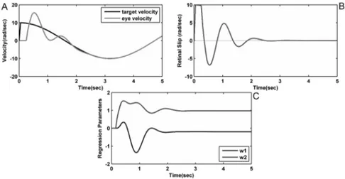
Figure 1.1.: Simulation results in case of a sinusoidal signal with angular frequency

of 1 rad s^(-1) and amplitude of 10 rad using Shibata and Schaal’s model. Here A and B show the time course of target and eye velocity and the retinal slip, respectively. After about 4 seconds the target velocity and the eye velocity are aligned and the values of the vector of regression parameters w reaches convergence (C) [-0.1987; 0.9751].

w in the angular frequency domain. The converging speed is slower than in humans

(Shibata et al. 2005), and if a new target dynamics is presented to the model, it is necessary to wait for the system converging, aside if this dynamics has been already presented or not. With the purpose to obtain a developmental model that can take into account previous experiences, in this work it has been supposed that it is possible to store the previously acquired weights, the regression coefficients. These values are placed in a memory block and then used to improve the converging speed of the model.

Fig. 1.2 shows that there is a direct relationship between the angular frequency of the target dynamics and the final regression coefficients calculated by the RLS al-gorithm. Such values depend only on the angular frequency of the target dynamics and on the configuration of the system. Instead, they are independent from the amplitude and the phase of the sinusoidal motion. In this work, a module storing the regression coefficients of already seen target motions has been added to Shibata and Schaal’s modeladded. Fig. 1.3 shows the proposed model block schema. The velocity information ( ˙v) are processed by the V1 and MT areas in order to extract the target slip on the retina ( ˙e). These operations are made by the Visual Process-ing module. The Estimator State module generates the target velocity estimation according to Equation 1.1 and it employs the position estimation by integrating the

(18)

Figure 1.2.: The graph shows the correlation between the values of regression

pa-rameters w and the angular frequency of sinusoidal target dynamics.

velocity information. The state vector (x) is sent to the Predictor that provides the next target velocity ( ˙x). The Inverse Dynamics Controller generates the necessary torque that allows the Eye Plant to reach the predicted velocity (Equation 1.6). In general, the system develops an internal representation, i.e. an Internal Model, of the external environment. The Internal Model, namely a memory block, has been added to recognize the target dynamics and to provide the correct weight values before the RLS algorithm. For this purpose, the regression coefficients are stored in a neural network, the Internal Model, for future presentation of learned target dynamics. The Predictor, shown in Fig. 1.3, is the RLS algorithm that minimizes the retinal slip, ˙e(t), adapting the regression coefficient according the Equation 1.4. The neural network inputs are a sample series of initial velocity values of the target dynamics and the outputs are the correct regression coefficients of the corresponding target dynamics. Such weights are sent to the predictor module in Equation 1.4 to guide the RLS algorithm to final values improving the converging speed. When the new values are ready from the network, it is necessary to wait for another cycle to verify the correctness of this prediction. If the retinal slip given by RLS is greater than the neural network one, the neural network output is used to predict the target velocity. In the other case, the RLS goes on learning the target dynamics, hence it is necessary to train the neural network on the new data. This behaviour is represented by the Selector module in block schema. Notes that the Predictor block in Fig. 1.3 provides a target velocity prediction that overcome the delay in the execution of the movement (∆3). The entire close loop delay has been fixed to ∆2=∆1+∆3. From

a neurophysiological point of view, the visual motion information follows the dorsal pathway and are processed by the primary visual cortex, MT and MST. This area provides the sensory information to guide pursuit movements but may not be able to initiate them. The FEF, in the pre-motor cortex, is more important for initi-ating pursuit and it is also related with associative memory (Chou and Lisberger

(19)

1.6 Implementation of the proposed model of smooth pursuit

Figure 1.3.: The figure shows a block schema of the proposed model of the smooth

pursuit eye movement. An internal model is added to Shibata and Schaal’s model to learn the target dynamics and a selector allows to recognize the best prediction between the internal model and the RLS predictor. The internal model is online trained by the values of the regression parameter vector when the RLS reaches convergence.

2004). Then, it is possible to suppose that the brain keeps motion information and use them to obtain a correct smooth pursuit eye movement based on own previous experience.

1.6. Implementation of the proposed model of

smooth pursuit

In the proposed model, a neural network has been added to associate a specific sequence of velocity values with the correct regression parameters. For this purpose, it has been used a simple multilayer perceptron (MLP) that maps half second of sampled target velocity (with sampling frequency of 20 Hz) onto corresponding weight values. This network has been developed with Neural Network Fitting Tool on MATLAB with 10 neurons in the input layer, 25 neurons in the hidden layer and 2 neurons in output layer that correspond with the two regression parameters of RLS algorithm. It uses the non linear activation sigmoid function with backpropagation learning rule. In accordance with neurophysiological studies, the model recognizes motion sequences and so it takes only half a second to provide the correct values. Moreover, when the learning is complete, it is possible to obtain correct values also with unknown angular frequency target motions. The model follows a developmental approach, therefore initially the neural network needs to learn by experience. The RLS algorithm learns the target dynamics and reaches convergence. The regression coefficients are used to train the neural network. When the neural network gives as

(20)

output a new predicted velocity value, the selector module has to compare this value with the real state of the target to verify the correctness of the prediction. So it has to wait one closed-loop delay for the new values of the target state. If the internal model prediction is better than the actual RLS output, the selector module changes the regression parameters in Equation 1.4 with the neural network output, otherwise it has to wait for the convergence of RLS and to use the regression parameter obtained for the learning of the neural network. The dimension of the input layer has been chosen from experimental trials. The velocity sample number needs to be a trade-off between the motion recognition accuracy (that needs large number of samples) and the system response velocity. Considering the specific system configuration it has been observed that 10 samples (0.5 sec at 20 Hz) are a good solution.

1.7. Experimental Results

The model represents the signal prediction of one axis because it has been proven that the horizontal axis is separate from the vertical axis (Grönqvist et al. 2006). To represent the other axis it is necessary to add another model like this one for the other component of the target dynamics. Moreover, the model predicts only the target velocity, so the position error reaches a constant value after the convergence of the system. In this work, all the learning experiments start from scratch, i.e. with all initial states including the weights of the learning system set to zero. The model was tested on sinusoidal target motions with the following dynamics:

x(t) = A ∗ sin(ωt + ϕ) (1.7)

Where x(t) is the target position (expressed in radians) at the time t and A is the amplitude of the dynamics. The angular frequency (ω) has been tested between 0.5 rad s−1 and 2.5 rad s−1 with 0.1 rad s−1 step. Moreover the model has been tested with angular phase between 0 rad and 2π rad with a π/4-rad step and with amplitude between 4 and 20 rad with a 1-rad step. Fig. 1.4 shows the results of an example of simulation with a sinusoidal motion target with angular frequency of 1 rad s−1: the final values of the vector w are -0.1987 and 0.9751. These values are independent from amplitude or phase of the sinusoidal trajectory. The vector of regression parameters is dependent only on the angular frequency of the sinusoidal motion and on the configuration of the system, like the entire closed loop delay. If the angular frequency changes, it will be necessary to wait that the model reaches the new steady state. With these configuration properties, the Schaal and Shibata’s model takes more than 4 seconds to perfectly cancel the retinal slip. In all exper-iments it has been taken into account, as converging speed, the time necessary for the vector of regression parameters to reach the stable state. For this purpose it

(21)

1.7 Experimental Results

Figure 1.4.: Simulation results in case of a sinusoidal target dynamics with angular

frequency of 1 rad s^(-1) and amplitude of 10 rad using the proposed model. Here A and B show the time course of target and eye velocity and the retinal slip respectively. After 0.8 second the values of the vector of regression parameters w are set to the final values (C) [-0.1987 0.9751] and the retinal slip reach zero just after this time.

has been chosen that the difference between elements of the vector of regression parameters and previous values of itself , e(k), must be less of 10^(-6).

e(k) = w(k) − w(k − 1) (1.8)

For example, for ω=1 rad s−1, A=10 rad; φ=0 the converging time is 6.75 sec. These values are strictly dependent on the initial conditions of the system and on the target dynamics. Fig. 1.5 shows the results of all simulation tests changing the amplitude in a range from 4 to 20 rad with a 1-rad step and the angular frequency in a range from 0.5 and 2.5 rad s−1 with fixed phase. Fig. 1.6 shows the results of all simulation tests changing the phase in a range from 0 rad and 2π rad with a π/4-rad step and angular frequency in a range from 0.5 and 2.5 rad s−1 with fixed amplitude. The converging speed increases as frequency and amplitude increase, moreover there is a periodic trend with the phase change. In the improved model it has been assumed that 10 steps are necessary (half a second with sampling frequency of 20 Hz) to recognize precisely the motion. The network outputs the vector of regression parameters and it is placed in Equation 1.4 for at least 5 seconds. The model corrects the prediction and the absolute value of retinal slip reaches steady state after 0.8 sec. When the new values are ready from the network, it is necessary to wait for another cycle to verify the correctness of this prediction so the final converging time is the sum of the time necessary to get 10 samples of target velocity (500 ms at 20 Hz), plus the time to verify that the prediction of neural network is better than the prediction coming from RLS (one closed loop delay, 200 ms) and

(22)

Figure 1.5.: Simulation results in case of a sinusoidal target velocity at several

am-plitude and angular frequency using Shibata and Schaal’s model. The converging time is between 5 and 10 seconds.

the time to move the eye to the correct predicted velocity (100 ms). In order to test the hypothesis that the model can recognise the initial value of the target dynamics, the neural network has been trained on a large training data set. It has been taken into account a sinusoidal target dynamics with the angular frequency included in a range from 0.5 and 2.5 rad s−1 with a 0.1-rad s−1 step. The neural network must give the correct value of the regression parameter vector aside from differences in the values of the amplitude and the phase of the sinusoidal target dynamics. So, for each angular frequency, 10 values have been taken (with sampling frequency of 20 Hz) of the target velocity (the derivative of the target position), considering the amplitude of the target position included between 5 and 15 rad with a 2.5-rad step, thus the maximum velocity considered is about 40 rad s−1. Moreover, it has been taken into account a different initial phase of the target dynamics in a range included between π/2 and π rad with π/16 rad step. It has been taken into account 945 (all combination of angular frequency, phase and amplitude) simulation results and the training set for the neural network is the 70% of this matrix. The 15% is used for the validation set and another 15% is used for the test set. The input matrices have dimension 10x945 and the output target has 2x945 elements. These values have been shuffled to increase the variability of the training set. The results of the learning are shown in Fig. 1.7. The best Mean Squared Error is 9.1844 exp−10. Fig. 1.8 shows the results of the model after the learning of the neural network in two different sinusoidal target dynamics. The figure shows that after 0.8 sec the model recognises the dynamics and gets out the correct values of the regression parameter vector aside the different condition in phase or in amplitude.

This work demonstrates that the smooth pursuit eye movement in humanoid robots can be modeled as a sensory-motor loop where the visual sensory input can be pre-dicted, and where the prediction can be improved by internal models that encode

(23)

1.7 Experimental Results

Figure 1.6.: Simulation results in case of a sinusoidal target velocity at several

phase and angular frequency using Shibata and Schaal’s model. The converg-ing time is between 5 and 9 seconds. The graph shows a periodic trend of the converging time with the phase change.

target trajectories already experienced by the system and that are built by learning. The proposed model includes a learning component that decreases the prediction time for a robotic implementation. The internal model is a feedforward artificial neural network that recognizes the initial sequence of target velocity and gives as output the correct values of the regression parameter vector. The neural network chosen for the internal model provides an improvement for the converging speed of the model but it leads to some considerations. First of all, the dimension of the hidden layer has been chosen a priori so it might be not optimal for another type of data. Secondly, the neural network requires more computational burden than the original model. Thirdly, it needs much memory for storing the training set of data. In the implementation described in the paper the convergence time reaches as low values as 0.8 seconds. As a reference, in the same implementation conditions, the convergence time of Schaal and Shibata’s model is more than 4 seconds. This system with this configuration is unable to predict complex dynamics like a sinu-soidal sum. Shibata et al. 2001 considered in their work these RLS limitations, but an improvement of the system like they suggested would not change the possibility presented here to take into account the converging results. Such results demonstrate that a memory based approach can improve the performance of the system. So it is possible to suggest that initially the smooth pursuit system needs to learn the target dynamics. During this phase it requires to use a large number of saccades to correct position errors. When the system has built its own Internal Model of the external environment, it uses its experience to rapidly obtain a zero-phase lag smooth pursuit.

(24)

Figure 1.7.: The graph shows the learning phase of the neural network. The Mean

Squared Error is less than 10^(-9) after 1000 epochs and is plotted for training set, validation set and test set of data.

Figure 1.8.: Simulation results in case of two sinusoidal target dynamics with

an-gular frequency of 1 rad s^(-1) and an amplitude of 10 rad and phase of π/2 (a, the grey line) and amplitude of 15 rad and phase of ¾ π (b, the black line) using the proposed model . Here A and B show the time course of target and eye ve-locity and the retinal slip respectively. After 0.8 second the values of the vector of regression parameters w are set to the final values (C) [-0.1987 0.9751] and the retinal slip reach zero just after this time independently from the differences of the amplitude and the phase of the target dynamics.

(25)

2. Smooth pursuit and saccades

2.1. Overview

The space-variant resolution of the retina requires efficient eye movements for cor-rect vision. Two forms of eye movements — saccades and smooth pursuit — enable us to fixate the object on the fovea. Saccades are high-velocity gaze shifts that bring the image of an object of interest onto the fovea. Saccades are fast eye movements (maximum eye velocity > 1000 deg/sec) that allow primates to shift the orientation of the gaze using the position error (difference between the target position and the eye position) (Leigh and Kennard 2004). The duration of the saccadic movement is very short (30-80ms), so they cannot be executed with continuous visual feedback. Smooth pursuit occurs when the eyes track a moving target with a continuous mo-tion, in order to minimize the image slip in the retina and make it perceptually stable (as described in chapter 1). Smooth pursuit movements cannot normally be generated without a moving stimulus although they can start a short moment before the target is expected to appear (Wells and Barnes 1998). The purpose of the work presented in this chapter is to investigate the applicability of a visual tracking model on humanoid robots in order to achieve a human-like predictive behavior. Rather than analyse the saccadic system as a separate module, the present work focuses on the predictive relationship between the smooth pursuit and the saccadic systems. Firstly, it has been analyzed the case of smooth pursuit tracking across occlusions (Falotico et al. 2009) where the tracking stops when the object is occluded an one or two saccades are made to the other side of the occluder to anticipate when and where the object reappears. Another critical case is called “catch-up” saccade, a particular combination of smooth pursuit and saccades that occurs when the track-ing error in position increases too much (Falotico et al. 2010). Both cases strictly depend on the predictive behaviours expressed by the smooth pursuit system. The described models have been implemented on the iCub robotic platform. Due to the fact that this platform has been taken into account for the robotic implementation of this and the other works, the session sec. 2.2 introduces the mentioned robot.

2.2. The iCub Robot

The RobotCub project has the twin goals of creating an open and freely-available humanoid platform, iCub, for research in embodied cognition, and advancing our

(26)

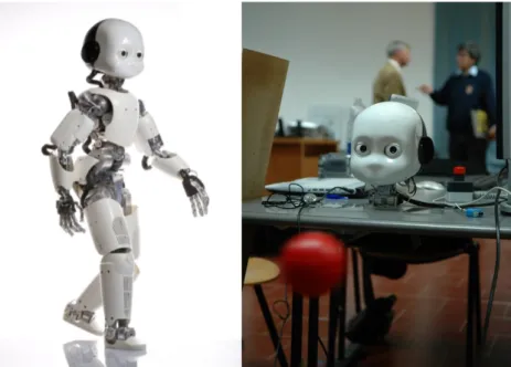
Figure 2.1.: The iCub robot has a physical size and shape similar to that of an

about three year-old child. The iCub head contains a total of 6 DOFs: neck pan, tilt and swing and eye pan (independent) and tilt (common).

understanding of cognitive systems by exploiting this platform in the study of cogni-tive development (Metta et al. 2010; Tsagarakis et al. 2007). To achieve this goal it has been planned to construct an embodied system able to learn: i) how to interact with the environment by complex manipulation and through gesture production & interpretation; and ii) how to develop its perceptual, motor and communication ca-pabilities for the purpose of performing goal-directed manipulation tasks. The iCub robot has a physical size and shape similar to that of an about three year-old child, and will achieve its cognitive capabilities through artificial ontogenic co-development with its environment (Fig. 2.1). The iCub has a total of 53 degrees of freedom orga-nized as follows: 7 for each arm, 8 for each hand, 6 for the head, 3 for the torso/spine and 7 for each leg. In order to guarantee a good representation of the human move-ments, the iCub head contains a total of 6 DOFs: neck pan, tilt and swing and eye pan (independent) and tilt (common) (Beira et al. 2006). The eyes cyclotor-sion was ignored because it is not useful for control, and similar image rotations are easily produced by software. The elevation/depression from both eyes is always the same in humans, in spite of the existence of independent muscles. Similarly, a single actuator is used for the robot eyes elevation (tilt). Eye vergence is ensured by independent motors. Data regarding accelerations, velocities and joint range of the oculomotor system of human babies are not available, and very few studies exist in the literature of psychology or physiology. Overall, the iCub dimensions are those of about three-year old human child, and it is supposed to perform tasks similar to those performed by human children. First, it has been used the small-est range of saccadic speeds as a reference and it has been used the ratio between

(27)

2.2 The iCub Robot

Figure 2.2.: The iCub simulator has been designed to reproduce, as accurately as

possible, the physics and the dynamics of the robot and its environment.

neck/eye velocity (14% − 41%) and acceleration (2% − 4%) as an important design parameter. The eyes mechanism has three degrees of freedom. Both eyes can pan (independently) and tilt (simultaneously). The pan movement is driven by a belt system, with the motor behind the eye ball. The eyes (common) tilt movement is actuated by a belt system placed in the middle of the two eyes. Each belt system has a tension adjustment mechanism. For the necessary acceleration and speed, the iCub has Faulhaber DC micromotors, equipped with optical encoders and planetary gearheads. In order to guarantee easy assembly and maintenance procedures, the mechanical system architecture is also completely modular, in such a way that it is possible to remove and replace a certain module, without having to disassemble the entire structure. For vision, the main sensory modality, two DragonFly cameras with VGA resolution and 30 fps are integrated in the head. These cameras are very easy to integrate because the CCD sensor is mounted on a remote head, connected to the electronics with a flexible cable. In this way, the sensor head is mounted in the ocular globe, while the electronics are fixed to a non-moving part of the eye-system. All motor control boards are specially designed to fit in the size constraints of the robot. They are all integrated in the head and connect to the remote com-puter with a CAN bus. To measure the head position (kinesthetic information), the motors have magnetic encoders, for calibration purposes and noting that the protection system drift in case of overload condition, absolute position sensors were applied to each neck joint. The simulator (Fig. 2.2) as stated has been designed to reproduce, as accurately as possible, the physics and the dynamics of the robot and its environment (Tikhanoff et al. 2008b;a). It has been constructed collecting data directly from the robot design specifications in order to achieve an exact replication of the iCub. This means same height, mass and d.o.f.. The iCub simulator was created using open source libraries. It uses ODE (Open Dynamics Engine) for

(28)

sim-ulating rigid bodies and the collision detection algorithms to compute the physical interaction with objects. ODE consists of a high performance library for simulat-ing rigid body dynamics ussimulat-ing a simple C/C++ API. The iCub Simulator allows controlling iCub robot in the position and in the velocity space, and it provides the encoder value of each motor. The iCub simulator uses YARP as its software archi-tecture. YARP (Yet Another Robot Platform ) software (described in (Metta and Fitzpatrick 2006; Fitzpatrick et al. 2008)) is the middleware software used by the iCub humanoid robot. It is worth mentioning that the iCub simulator is one of the few that attempts to create 3D dynamic robot environment capable of recreating complex worlds and fully based on non-proprietary open source libraries.

2.3. Predictive tracking across occlusions

The smooth pursuit is complicated by the fact that the initial visual processing in the human brain delays the stimulus by approximately 100 ms before it reaches the visual cortex (Wells and Barnes 1998; Fukushima et al. 2002). When the pursued object is occluded, the smooth eye movements get effectively interrupted. Subjects switch gaze across the occluder, with saccades, to continue tracking (von Hofsten et al. 2007). This is valid for visual tracking in adults (Lisberger et al. 1987; Kowler 1990) and in infants (Rosander and von Hofsten 2004). Infants react differently from adults to occlusions of the object. Adults always predict the reappearance and their gaze arrives at the opposite side of the occluder slightly before the object. Infants can simply maintain a representation of the object motion while the object is occluded and shift gaze to the other side of the occluder when the conceived object is about to arrive there. In support of this alternative are the findings that object velocity is represented in the frontal eye field (FEF) of rhesus monkeys during the occlusion of a moving object (Barborica and Ferrera 2003). An interesting paper about occlusions and eye movements is proposed by Zhang and colleagues (Zhang et al. 2005). They describe a real-time head tracking system, formulated as an active visual servo problem based on the integration of a saccade and a smooth pursuit process.

2.4. The proposed model for occlusions

This work proposes the integration of different systems in order to obtain a human like behavior of a predictive smooth pursuit of a dynamic target, with saccadic shift of gaze in case of occlusions. The presented model is able to predict target trajecto-ries that present a second order dynamics also in presence of temporary occlusion. It is possible to extend this model to cope with more complex target motions with nonlinear dynamics as suggested in (Shibata and Schaal 2001). (Fig. 2.3) shows the entire system model. The model is basically an extension of the model presented

(29)

2.4 The proposed model for occlusions

Figure 2.3.: If the object disappears behind the occluder a event of occlusion is

notice and another module starts to detect the edges in the image to find where the object will reappear. At this point the saccade generator module repeats the prediction of the target dynamics until the predicted position is equal to the edge detected from the previous module.

by the author in Zambrano et al. 2010 and described in sec. 1.5. The first module is the visual tracker that allows rapid recognition of the object and provides its posi-tion in eye coordinates to the next modules. If the object is visible the informaposi-tion about target is processed and the smooth pursuit is executed. The smooth pursuit system requires only measurements of the retinal slip (the target velocity on the retina) to estimate the next target velocity. This information is obtained from the difference of the target position in eye coordinates sent by the tracking module, with respect to the sampling time of the cameras. When the system learns to predict the target dynamics the regression vector values reach convergence and the internal model stores these values. This part of the model basically follows the description presented in sec. 1.5. Regarding the behaviour expressed during occlusions, if the object disappears behind the occluder the tracking module stops sending data and another module starts to detect the edges in the image to find where the object will reappear. At this point the saccade generator module repeats the prediction of the target dynamic by a reiteration of Equation 1.5 with the complete regression matrix, as follows: Y(t + 1) = " 1 ∆t w1 w2 # Y(t) (2.1)

(30)

Where ∆t is the sampling time of the cameras and Y(t) represents the velocity and the position of the target. In order to obtain a long term prediction, the current state Y(t) has to be set equal to the previous iteration of Equation 2.1. The 2.1 is repeated until the predicted position is equal to the edge detected from the previous module. In this way it is possible to obtain the position and the velocity of the target reappearance. The robot switches gaze saccadicly across the occluder to continue tracking and arrives at the opposite side of the occluder slightly before the object. In Fig. 2.4 are shown the results obtained from a simulation of this model on MATLAB Simulink for a sinusoidal dynamics with angular frequency of 1 rad/sec and amplitude of 20 rad. The occlusion range was chosen between -10 rad and 10 rad. In Fig. 2.4 (top) are shown the eye position and the target position. When the target goes behind the occluder, the eye rapidly reaches the exact reappearance point predicted. In Fig. 2.4 (down) the eye velocity has a peak on correspondence with the saccadic movement, then it goes to zero until target reappearance. The velocity of the saccadic movement reaches 300 rad/sec.

2.5. Robotic implementation

To emulate the gazing behaviour of humans in an experiment when the object of in-terest undergoes total occlusions, we use a method for object detection and tracking with built-in occlusion detection. Two properties of the tracking system are impor-tant for this work: it must be able to detect transitions between the states of full visibility and occlusions of the tracked object and it must be able to initialize au-tonomously the tracker when the object of interest reappears after an occlusion. The detection of the aforementioned transitions is important for our purposes because it corresponds to the events when humans toggle their eye movement behaviour from smooth pursuit to saccadic. We use the tracking system described in (Taiana et al. 2010; 2008), exploiting the behaviour of the likelihood values it computes whens the object of interest is partially occluded. The tracking system we use is based on Particle Filtering methods and exploits knowledge on the shape, color and dynamics of the tracked object. Each particle in the filter represents a hypothetical state for the object, composed of 3D position and velocity. Particles are weighted according to a likelihood function. To compute the likelihood of one particle we first place the points of the shape model around the 3D position encoded in the particle, with respect to the camera. Then we project these points onto the image plane obtaining two sets of 2D points. The sets of 2D points lie on the image on the inner and outer boundary of the silhouette that the tracked object would project if it were at the hypothetical position. The idea is that the color and luminance differences be-tween the sides of the hypothetical silhouette are indicators of the likelihood of the corresponding pose. Object-to-model similarity positively influences the likelihood, while object-to-background similarity contributes to likelihood in the opposite di-rection. When the object of interest is fully visible, the likelihood estimated by the

(31)

2.6 The visual tracking model

filter as a whole is high. When the object gradually becomes occluded, the tracker continues working, but the estimated likelihood drops, only to rise again when the object reappears. The observation model we use enables us to detect occlusions and reappearance events just by setting a threshold on the likelihood value and by reini-tializing the tracker, effectively running a detection process, each time the likelihood is below that threshold. The initialization is performed by generating a new particle set, sampling a predefined Gaussian distribution.

Beyond the simulations we have performed results on the real robotic platform iCub (described in sec. 2.2). A known target (a blue ball) is suspended from the ceiling with a string. Once it is put into periodic oscillation, the robot starts estimating and tracking the ball trajectory. It uses the predicted velocity to command the eye motions. Suddenly, an occluder is put close to the ball. At moderate amounts of occlusions, the robot still detects the ball and keeps tracking it. When the occlusion is almost complete, the smooth pursuit tracking stops and the robot estimates when and where the ball will reappear, preparing a saccade. The saccade happens at the onset of reappearance and the eyes are already centered at the target and ready to keep tracking it (Falotico et al. 2009).

2.6. The visual tracking model

The space-variant resolution of the retina requires efficient eye movements for correct vision. Saccades are fast eye movements (maximum eye velocity > 1000 deg/sec) that allow primates to shift the orientation of the gaze using the position error (difference between the target position and the eye position) (Leigh and Kennard 2004). The duration of the saccadic movement is very short (30-80ms), so they cannot be executed with continuous visual feedback. The saccade generation consists in a sensorimotor transformation from visual space input to the motor command space. That transformation involves many brain areas from the superior colliculus (SC) to the cerebellum. Some of these areas are similar to those involved in the smooth pursuit generation (de Xivry 2007). Usually smooth pursuit is executed for predictable target motion rather the saccades are used in correspondence of static target. In case of moving target the oculomotor system uses a combination of the smooth pursuit eye movement and saccadic movement, namely “catch up” saccades to fixate the object of interest. Recent studies investigate the mechanisms underlying the programming and the execution of catch-up saccades in humans (de Brouwer and Missal 2001; de Brouwer et al. 2002a;b).

The model presented in sec. 1.5 (and Zambrano et al. 2010) is able to predict target trajectories that present a second order dynamics. It is possible to extend this model to cope with more complex target motions with nonlinear dynamics as suggested in sec. 2.4 (Falotico et al. 2009). This model is composed by a saccade generator system and a predictive model of smooth pursuit eye movement. The smooth pursuit controller has been proposed by Shibata (Shibata and Schaal 2001). This controller

(32)

learns to predict the visual target velocity in head coordinates, based on fast on-line statistical learning of the target dynamics. This model has been modified to improve its convergence speed by using a memory based internal model that stores the already seen target dynamics (Zambrano et al. 2010). Fig. 1.3 shows the smooth pursuit model block schema. The Estimator State module generates the target velocity estimation and computes position by integrating the velocity information. The state vector is used by the Predictor to compute the target velocity in the next time step. The Inverse Dynamics Controller generates the necessary torque force that allows the Eye Plant to reach the predicted velocity. This controller corresponds to the low-level velocity controller of the robot. The control model consists of three subsystems: a RLS (Ljung and Soderstrom 1987) predictor (see sec. 1.4) mapped onto the MST, which receives the retinal slip, i.e. target velocity projected onto the retina, with delays, and predicts the current target motion; the inverse dynamics controller (IDC) of the oculomotor system, mapped onto the cerebellum and the brainstem; and the internal model that recognizes the already seen target dynamics and provides predictions that are used alternatively to the RLS predictor. The third part is based on the fact that there is a direct relationship between the angular frequency of the target dynamics and the final weights of the model. Such values depend only on the angular frequency of the target dynamics and on the configuration of the system, being independent from the amplitude and the phase of the sinusoidal motion. A memory block (Internal Model) recognizes the target dynamics and it provides the correct weights values before the RLS algorithm. For this purpose, such weight values are stored in a neural network (MLP) for future presentation of learned target dynamics. The neural network outputs are the correct weight values of the corresponding target dynamics. Such weights are set to the predictor module in order to guide the RLS algorithm to final values improving the converging speed (see sec. 1.5 and Zambrano et al. 2010). Concerning the Saccade Generator block, it has been implemented the results provided from recent studies (de Brouwer and Missal 2001; de Brouwer et al. 2002a;b). These studies show that the smooth pursuit motor command is not interrupted during catch-up saccades. Instead the pursuit command is linearly added to the saccade. From experimental data analysis it has been also shown that there is a specific equation that can generate a correct saccade, taking into account both position error e(t) and retinal slip ˙e(t):

ESamp = 1 ∗ e(t) + (0.1 + Sdur) ∗ 0.77 ∗ ˙e(t) (2.2)

Where ESamp is the exact amplitude of the saccade that will catch the moving

target and Sdur is an estimate average saccade duration (= 0.074). Although the

experimental results show that the final position error is not always cancel out by the catch-up saccade and that it is influenced by retinal slip (de Brouwer and Missal 2001; de Brouwer et al. 2002a), for this robotic implementation it has been used the exact formula. Moreover the saccade amplitude is converted in a velocity profile in order to keep the same velocity control using for the smooth pursuit system and

(33)

2.7 Results

to obtain the linear adding of the smooth pursuit and saccadic command. The mechanism underling the decision to switch from the smooth pursuit system to the saccadic system has been also studied (de Brouwer et al. 2002b). What it has been found is that the oculomotor system uses a prediction of the time at which the eye trajectory will cross the target, defined as the eye crossing time TXE. This value

has been defined as the ration between the opposite of the position error e(t) and retinal slip ˙e(t) :

TXE = −

e(t)

˙e(t) (2.3)

This time is evaluated 125 ms before saccade onset due to the visual system delay. On average, for between 40 and 180 ms no saccade is triggered and target tracking remains purely smooth. In contrast, if is smaller than 40 ms and larger than 180 ms, a saccade is triggered after a short latency. With regard to the proposed implemen-tation the Equation 2.3 for the eye crossing time poses two problems. First of all, the equation presents a discontinuity when the retinal slip is null. Although this case, probably never happens in real systems, in principle, the smooth pursuit controller tries to reduce the retinal slip as much as possible. Thus the trigger system will command for a saccade even if it is not necessary. The second problem connected with the previous, is that the robotic system has some intrinsic limits firstly due to the noise added to the measure of the position error from the cameras. Others sources of errors are the accuracy of the motor system and the noise on the encoder. Thus the accuracy of the entire system is not less 3 degrees. For these reasons it has been added a threshold value for which the saccade will be not generated if the absolute value of the position error is smaller than 3 degree. This threshold could be modified depending on the characteristic of the specific robotic system.

2.7. Results

The model has been tested on the iCub Simulator and on Matlab Simulink. Both implementation results showed in the figures below, try to reproduce experiments on humans (described in de Brouwer et al. 2002b). These experiments aim at studying the interaction between saccades (catch-up saccades) and smooth pursuit. Fig. 2.6 show examples of responses to unexpected changes in target motion. In particular they show a typical response to an increase in target velocity between two ramps. Smooth pursuit system is able to cancel out the retinal slip during the first ramp, but has no influence on the position error on the retina. So, when the second ramp occurs, the position error increases and one or more corrective saccades are elicited to reach the target. The Fig. 2.6 is the result of a test executed on the iCub Simulator (described in sec. 2.2). The implementation confirms expected results,

(34)

according to human experimental data (de Brouwer et al. 2002b). The model has been tested on sinusoidal target motions (already tested as input in Equation 1.7). Fig. 2.7 shows the results of an example of simulation with a sinusoidal motion target with frequency of 0.2 Hz and 0.4 Hz. The target position and the eye position are aligned for five seconds, when the target position follows an already known sinusoidal motion. After this time the frequency of the sinusoidal target motion is doubled. The position error increases and some saccades are elicited. Saccades correspond to peaks in the position error time course. The model is able to cancel the retinal slip with the smooth pursuit and the position error with catch-up saccades. Preliminary tests have been executed on the iCub robot. The model has been tested on sinusoidal target motions with the dynamics described in Equation 1.7. The tracking algorithm used is based on Particle Filtering method (Taiana et al. 2008; 2010). Fig. 2.8 shows the results of an example of simulation with a sinusoidal motion target with frequency of 0.5Hz. The number of saccade elicited is greater than the number of saccade elicited in the same test executed on the iCub simulator, because of the noise. The position error, after an initial phase, decreases and after 5 seconds is almost canceled.

This work presents a model and a robotic implementation to address the problem of tracking visual targets with coordinated predictive smooth pursuit and saccadic eye movements, like in humans. The oculomotor system uses prediction to anticipate the future target trajectory during smooth pursuit. When the object motion is unpredictable there is an accumulation of retinal error that is compensated by catch-up saccades. These movements are executed without visual feedback and in order to achieve better performance they have to take in account the retinal slip.

(35)

2.7 Results

Figure 2.4.: The simulation results of the eye position and the target position

(top) for a smooth pursuit tracking with occlusion of a sinusoidal target dynamics with angular frequency of 1 rad/sec and amplitude of 20 rad. The gaze sac-cadiclymoves across the occluder to continue tracking and arrives at the opposite side of the occluder slightly before the object. The eye velocity (down) has a peack on correspondence with the saccadic movement, then goes to zero until target reappearance.

Figure 2.5.: The model schema is composed by a saccade generator system and a

(36)

Figure 2.6.: Example of the responses to unexpected changes in target velocity

between two ramps

Figure 2.7.: A smooth pursuit trial, for which the combination of retinal slip and

(37)

2.7 Results

Figure 2.8.: Simulation on iCub robot of response to a sinusoidal motion of the

(38)

(39)

3. The gaze control

3.1. Overview

Space-varinat resolution retina imposes that when we want to examine an object in the world, we have to move the fovea to it. The gaze system performs this function through two components: the oculomotor system, which moves the eyes in the orbit, and the head movement system, which moves the orbits in space (Kandel et al. 2000). The gaze system also prevents the image of an object from moving on the retina. It keeps the eye still when the image is still and stabilizes the image when the object moves in the world or when the head itself moves. As described in chapter 1 the smooth pursuit system keeps the image of a moving target on the fovea. While the saccadic system shifts the fovea rapidly to a visual target in the peripheryn (see chapter 2). Vestibulo-ocular movements hold images still on the retina during brief head movements and are driven by signals from the vestibular system. Optokinetic movements hold images during sustained head rotation and are driven by visual stimuli. Finally, there are times that the eye must stay still in the orbit so that it can examine a stationary object. Thus, another system, the fixation system, holds the eye still during intent gaze. This requires active suppression of eye movement. When we look at an object of interest a neural system of fixation actively prevents the eyes from moving.

The foundations of cognition are built upon the sensory-motor loop - processing sensory inputs to determine which motor action to perform next. The human brain has a huge number of such loops, spanning the evolutionary timescale from the most primitive reflexes in the peripheral nervous system, up to the most abstract and inscrutable plans. This chapter, complete the loop of the gaze control, by an-alyzing the learning mechanisms that govern its behavior. At the subcortical level, the cerebellum and basal ganglia are the two major motor control areas, each of which has specially adapted learning mechanisms. The basal ganglia are special-ized for learning from reward/punishment signals, in comparison to expectations for reward/punishment, and this learning then shapes the action selection that the organism will make under different circumstances (selecting the most rewarding ac-tions and avoiding punishing ones). This form of learning is called reinforcement learning. The cerebellum is specialized for learning from error, specifically errors be-tween the sensory outcomes associated with motor actions, relative to expectations for these sensory outcomes associated with those motor actions. Thus, the cerebel-lum can refine the implementation of a given motor plan, to make it more accurate,

(40)

efficient, and well-coordinated. Therefore we can say that the basal ganglia help to select one out of many possible actions to perform, and the cerebellum then makes sure that the selected action is performed well. A typical example of the role of the cerebellum in the gaze control is the VOR/OKR system.

3.2. The VOR/OKR system

This work is focused on oculomotor control, in particular in one of the most basic and phylogenetically oldest functions of oculomotor control: the visual stabilization. Since the oculomotor system resides in a moving head, successful visual perception requires that retinal images remain constant, at least for the time necessary for ac-curate analysis. The head motion is recognized by the oculomotor system and it knows how much to move the eyes to compensate for the head movement in order to maintain clear vision. The head motion is derivable from visual information be-cause when the head moves the image of the world also moves on the retina. It is also possible to derive head velocity from proprioceptive systems of the neck and body. However, these sensory mechanisms are too slow. In contrast, the hair cells of the vestibular system sense head acceleration directly, and this sensing in turn allows those reflexes (that require information about head motion) to act efficiently and quickly. Due to the latencies of the oculomotor system, however, many evi-dence suggest that the brain, and in particularly the cerebellum, uses learning to overcome these delays and to obtain perfect stabilization (Ito 1984). The state of the art of these system models provides basically two different approaches to the problem of the modeling of this behavior. In one case (Shibata and Schaal 2001), Shibata and Schaal suggest the idea of feedback error learning (FEL) as a biologi-cally plausible adaptive control concept (Kawato 1990). In this way they propose biomimetic oculomotor controller with accurate control performance and very fast learning convergence for a nonlinear oculomotor plant with temporal delays in the feedback loop. This model will be henceforward referred as FEL model. In an-other case (Porrill et al. 2004) Dean, Porrill and Stone propose an algorithm for the cerebellum, called decorrelation control, that offers the possibility of reconciling sen-sory and motor views of cerebellar function. The algorithm learns to compensate for the oculomotor plant by minimizing correlations between a predictor variable (eye-movement command) and a target variable (retinal slip), without requiring a motor-error signal. This model will be henceforward referred as decorrelation model. From biological point of view, in the VOR movement there are evidences of adaptive behavior (Ito 1984). By manipulation of the retinal slip using magnifying spectacles the ratio between eye and head velocity (VOR gain) changes after a certain learning time. This adaptation involves the vestibular cerebellum area that participates also in the Opto-Kinetic Response (OKR). The OKR reflex is another eye movement responsible of the stabilization of images from the retinal slip information. The retinal slip based feedback control loop is too late (80-100 ms) to fix the image on the