A sample selection model for unit and item nonresponse in cross-sectional surveys

A sample selection model for unit and item nonresponse

in cross-sectional surveys

Giuseppe De Luca Franco Peracchi

CEIS Tor Vergata - Research Paper Series, Vol.

33 , No. 99 , March 2007

This paper can be downloaded without charge from the Social Science Research Network Electronic Paper Collection:

http://papers.ssrn.com/paper.taf?abstract_id=967391

CEIS Tor Vergata

R

ESEARCH

P

APER

S

ERIES

A sample selection model for unit and

item nonresponse in cross-sectional surveys

∗

Giuseppe De Luca and Franco Peracchi

University of Rome “Tor Vergata”

This version: November 2006

Abstract

We consider a general sample selection model where unit and item nonresponse simulta-neously affect a regression relationship of interest, and both types of nonresponse are poten-tially correlated. We estimate both parametric and semiparametric specifications of the model. The parametric specification assumes that the errors in the latent regression equations follow a trivariate Gaussian distribution. The semiparametric specification avoids distributional as-sumptions about the underlying regression errors. In our empirical application, we estimate Engel curves for consumption expenditure using data from the first wave of SHARE (Survey on Health, Aging and Retirement in Europe).

Keywords: Unit nonresponse, item nonresponse, cross-sectional surveys, sample selection models, Engel curves.

JEL classification: C14, C31, C34, D12

∗_{We thank Chuck Manski, Frank Vella and seminar participants at Northwestern and UCL for helpful comments.}

Financial support for this research was provided through the European Community’s Program ‘Quality of Life’ under the contract No. QLK6-CT-2002-002426 (AMANDA). This paper is based on data from the early Release 1 of SHARE 2004, which is preliminary and may contain errors that will be corrected in later releases. The SHARE data collection has been primarily funded by the European Commission through the 5th framework program (project QLK6-CT-2001-00360 in the thematic program ‘Quality of Life’). Additional funding came from the US National Institute on Aging (U01 AG09740-13S2, P01 AG005842, P01 AG08291, P30 AG12815, Y1-AG-4553-01 and OGHA 04-064). Data collection in Austria (through the Austrian Science Fund, FWF) and Switzerland (through BBW/OFES/UFES) was nationally funded.

1

Introduction

Nonresponse is a very important source of nonsampling errors in sample surveys. A distinction is usually made between two forms of nonresponse: unit and item nonresponse. Unit nonresponse occurs when eligible sample units fail to participate to a survey because of failure to establish a contact, or explicit refusal to cooperate. Item nonresponse occurs instead when responding units do not provide useful answers to particular items of the questionnaire.

The relevance of distinguishing between unit and item nonresponse is twofold. First, data users can improve model specification, because different information is usually available for studying the two types of nonresponse. In fact, the information available to study unit nonresponse is usually confined to the information obtained from the sampling frame or the data collection process, whereas the additional information collected during the interview can be used to study item nonresponse. Second, understanding the different types of error generated by unit and item nonresponse plays a key rule at the survey design stage, where resources have to be allocated efficiently to reduce nonresponse errors. For instance, improving incentive schemes and follow-up procedures can help reduce unit nonresponse, while reducing the complexity of the questionnaire can help reduce item nonresponse.

For panel surveys, one can also distinguish a particular form of unit nonresponse, namely sample attrition. This occurs when a responding unit in one wave of the panel drops out in a subsequent wave. In this paper, we are mainly concerned with problems of nonresponse in cross-sectional surveys or, equivalently, in the first wave of panel surveys. Response rates in the first wave of a panel are typically much lower than in subsequent waves. For example, the overall household nonresponse rate in the first wave of the European Community Household Panel, a large longitudinal survey of the European population, is about 30 percent, whereas the overall household attrition rate in the next two waves is about 10 percent (Eurostat 1997). Despite its importance, however, response rate in the first wave has received little attention relative to panel attrition, largely because of the lack of information on unit nonrespondents.

One crucial issue in studying both unit and item nonresponse is establishing whether or not the mechanism generating missing observations is random. Following Rubin (1976), we distinguish between three missing data mechanisms: missing completely at random (MCAR), missing at ran-dom (MAR), and not missing at ranran-dom (NMAR). A mechanism is MCAR if missingness does not depend on the values of the variables in the data matrix. A mechanism is MAR if, after condi-tioning on a set of observed covariates, there is no relation between missingness and the observed

outcomes. A mechanism is NMAR if missingness and the observed outcomes are related even after conditioning on the set of observed covariates. When mechanisms underlying (unit or item) non-response are NMAR, ignoring nonnon-response errors or relying on the MAR assumption may lead to invalid inference about population parameters of interest.

An important strategy in order to reduce nonresponse errors consists of planning preventive measures to cope with nonresponse at the survey design stage. Well-designed surveys aim to reduce unit nonresponse rates by choosing the most appropriate fieldwork period, interview mode, interviewer training, follow-up procedures and incentive schemes. Other aspects of the questionnaire design, like length of the interview, wording of the questions and their reference period, are more likely to affect item nonresponse rates. Empirical studies by Groves and Couper (1998), Groves et al. (2002), O’Muircheartaigh and Campanelli (1999) and Riphahn and Serfling (2002), show that all these aspects of survey design are crucial to explain the response rates achieved in sample surveys.

Unfortunately, despite the preventive measures adopted for minimizing nonresponse errors, re-sponse rates are rarely close to 100 percent. This explains why most of the survey nonrere-sponse literature focuses on the development of statistical methods for ex-post adjustments of nonresponse errors (see Lessler and Kalsbeek 1992, and Little and Rubin 2002). Weighting adjustment meth-ods, which involve the assignment of weights to sample respondents in order to compensate for their systematic differences relative to nonrespondents, have been traditionally used to deal with problems of unit nonresponse, whereas imputation procedures, which aim to fill in missing values to produce a complete dataset, have been traditionally used to deal with problems of item nonre-sponse. Although ex-post adjustment techniques have reached a high level of sophistication, such methods commonly assume that the missing data mechanism is MAR, and they do not generally allow compensating simultaneously for errors due to unit and item nonresponse.

This paper differs from previous studies in two respects. First, problems of selectivity due to unit and item nonresponse are analyzed jointly. Second, missing data mechanisms underlying the different types of nonresponse are allowed to be NMAR. In particular, we analyze a general sam-ple selection model where unit and item nonresponse can jointly affect a regression relationship of interest, and the two types of nonresponse can be correlated. Attention focuses on two alternative specifications of the model, one parametric and the other semiparametric. In the parametric spec-ification, errors in the two selection equations (one for unit and one for item nonresponse) and in the equation for the outcome of interest are assumed to follow a trivariate Gaussian distribution.

In the semiparametric specification, we avoid distributional assumptions about the errors in the three equations. After discussing issues related to identification and estimation of the two kinds of model, we provide an empirical application by using data from the first wave of SHARE (Survey on Health, Aging and Retirement in Europe), a survey conducted in 2004 across eleven European countries. The aim of this analysis is to investigate the potential selectivity associated with unit and item nonresponse in the estimation of Engel curves for food consumption at home and total nondurable consumption.

The remainder of the paper is organized as follows. Section 2 formalizes the motivation of this study, and presents a general framework to analyze problems of unit and item nonresponse. Sections 2.1 and 2.2 consider problems of identification and estimation of the parametric and semiparametric model respectively. Section 3 presents our data. Section 4 presents our empirical results. Finally, Section 5 summarizes our main findings and offers some conclusion.

2

The statistical model

In what follows, we are interested in estimating the conditional mean function of a random outcome by using data from a survey. Initially, a set of n units is drawn at random from the population of interest. Nonresponse may then select the sample at two stages. First, unit nonresponse may

reduce the sample size to n1 < n responding units. Second, item nonresponse may further reduce

the number of usable observations to n2 < n1. This loss of observations causes an efficiency loss

relative to the ideal situation of complete response. This efficiency loss needs not be the main concern, however, because lack of independence between the missing data mechanism and the outcome of interest may also generate selectivity in the observed sample and may lead to biased estimates of the population parameters.

To formalize the statistical problem, we consider a sequential framework where individuals first decide whether to participate to the survey. Given participation, they then decide whether to

answer a specific item of the questionnaire. Thus, the indicator of unit response, Y1, is always

observed, the indicator of item response, Y2, is only observed for the units that agree to participate

to the survey, and the response process is completely described by two elements: the probability of

unit nonresponse, π0 = Pr{Y1 = 0}, and the probability of item nonresponse conditional on unit

response, π_{0|1 = Pr{Y}2 = 0 | Y1 = 1}. Our objective is to obtain consistent estimates of the mean

function of the outcome of interest Y3 (conditional on covariates) allowing for selectivity generated

By the law of iterated expectations1

E(Y3) = π0E(Y3| Y1 = 0) + (1 − π0)[π_0|1E(Y3| Y1= 1, Y2 = 0)+

+ (1 − π0|1) E(Y3| Y1= 1, Y2= 1)].

(1)

The sampling process identifies π0, π_0|1 and E(Y3| Y1 = 1, Y2 = 1) but not E(Y3| Y1 = 0) and

E(Y3| Y1 = 1, Y2 = 0). Hence, in the absence of additional information, E(Y3) is not identifiable.

The assumption that both unit and item nonresponse are MAR is convenient because it implies

that E(Y3| Y1= 1, Y2 = 1) = E(Y3), which enables one to directly exploit the information contained

in the subsample of fully responding units. If this assumption does not hold and estimates of

E(Y3| Y1 = 1, Y2 = 1) are used to estimate E(Y3), then the overall nonresponse bias is

E(Y3| Y1 = 1, Y2 = 1) − E(Y3) = π0[E(Y3| Y1 = 1) − E(Y3| Y1 = 0)]+

+ π_0|1[E(Y3| Y1 = 1, Y2= 1) − E(Y3| Y1= 1, Y2 = 0)].

(2)

Thus, the overall nonresponse bias depends on two separate components, respectively proportional to the probability of unit nonresponse and the probability of item nonresponse conditional on

unit response. The overall nonresponse bias is zero when π0 = π0|1 = 0 (neither unit nor item

nonresponse), or E(Y3| Y1 = 1) = E(Y3| Y1= 0) and E(Y3| Y1 = 1, Y2 = 1) = E(Y3| Y1= 1, Y2= 0)

(both unit and item nonresponse are MAR). Equation (2) makes it clear that there is also a third case in which the overall nonresponse bias is zero, namely when the bias components due to unit and item nonresponse have opposite sign and offset each other.

A simple way of allowing for differential selectivity effects of unit and item nonresponse is to adopt the following straightforward generalization of the classical sample selection model of Heckman (1979)

Y_j∗ = μj+ Uj, j = 1, 2, 3, (3)

Y1 = 1{Y1∗≥ 0}, (4)

Y2 = 1{Y2∗≥ 0}, if Y1 = 1, (5)

Y3 = Y3∗, if Y1Y2 = 1, (6)

where the Y_j∗, j = 1, 2, 3, are latent continuous random variables representing, respectively, the

propensity to participate to the survey, the propensity to answer to the item of interest, and the

outcome variable in the uncensored sample, and the Uj are regression errors with zero mean. The

μj are assumed to depend linearly on a kj-vector of fully observable exogenous variables Xj, that is,

1

μj = αj+ βj>Xj, j = 1, 2, 3, where αj and βj are unknown parameters to be estimated. The latent

variables Y∗

j are related to their observed counterparts Yj through the observation rules (4)—(6),

where 1{A} is the indicator function of the event A.

The primary interest of the analysis is estimation of the parameters in μ3 from the sub-sample

of fully observed units, for which

E(Y₃∗_{| Y}1Y2 = 1) = μ3+ σ3E(U3| U1> −μ1, U2> −μ2). (7)

If any of the two nonresponse mechanisms is NMAR, then the conditional expectation on the right hand side of (7) is different from zero, and traditional estimation methods, sach as ordinary least squares, lead to inconsistent estimates of the parameters of interest. Consistent estimation can be based on simple generalizations of the classical Heckman two-step procedure. Parametric and semiparametric versions of this procedure are presented in Sections 2.1 and 2.2 respectively. In both

cases, point identification of E(Y3) is achieved by restricting the shape of the joint distribution of

(Y1, Y2, Y3).

Although unavoidable if one seeks point identification, assumptions about the shape of the joint

distribution of (Y1, Y2, Y3) may not be entirely convincing, especially if they cannot be tested. When

the lack of credible assumptions about the response process prevents point identification of E(Y3),

partial identification in the sense of Horowitz and Manski (1998) and Manski (2003) would still be

possible if one could bound E(Y3| Y1 = 0) and E(Y3| Y1 = 1, Y2 = 0) in (1). Specifically, suppose

that E(Y3| Y1 = 0) can take any value in the interval [a0, a1], whereas E(Y3| Y1 = 1, Y2 = 0) can

take any value in the interval [b0, b1]. Then, E(Y3) must necessarily lie in the interval H = [c0, c1],

where

c0= π0a0+ (1 − π0)[π0|1b0+ (1 − π0|1) E(Y3| Y1 = 1, Y2 = 1)],

c1= π0a1+ (1 − π0)[π_0|1b1+ (1 − π_0|1) E(Y3| Y1 = 1, Y2 = 1)],

whose width is equal to

c1− c0 = π0(a1− a0) + (1 − π0)π_0|1(b1− b0).

When Y3 is non-negative, as in the empirical example in Section 4, it is natural to choose a0= b0=

0. The resulting bounds of the identification region for E(Y3) are

c0= (1 − π0)(1 − π_0|1) E(Y3| Y1 = 1, Y2 = 1)],

c1= π0a1+ (1 − π0)[π_0|1b1+ (1 − π_0|1) E(Y3| Y1 = 1, Y2 = 1)],

and the width of the identification region is c1− c0 = π0a1+ (1 − π0)π_0|1b1. Even in this case,

however, credible values for a1 and b1 are not easily found (unless when Y3 is a 0-1 indicator, in

2.1

Parametric estimation

Our parametric framework assumes that the latent regression errors follow a trivariate Gaussian distribution with zero mean and correlation matrix

Σ = ⎡ ⎣ ρ112 ρ112 ρρ1323 ρ13 ρ23 1 ⎤ ⎦ .

We also normalize the variances of U1 and U2 to one in order to identify the coefficients of the

binary response equations.

In this parametric setting, the vectors β = (β1, β2, β3) and α = (α1, α2, α3) of regression

para-meters can be estimated consistently through the two-step procedure proposed by Poirier (1980) and further developed by Ham (1982). Here, we slightly modify their procedure in order to account

for partial observability of Y2. The procedure exploits the fact that, under our set of assumptions,

we have the explicit representation

E(U3| U1 > −μ1, U2 > −μ2) = ρ13λ1(θ) + ρ23λ2(θ), (8)

where θ = (α1, α2, β1, β2, ρ12), the λj(θ) are bias correction terms given by

λ1(θ) = φ(μ1) Φ(σ−1(μ2− ρ12μ1)) Φ2(μ1, μ2; ρ12) , λ2(θ) = φ(μ2) Φ(σ−1(μ1− ρ12μ2)) Φ2(μ1, μ2; ρ12) ,

σ = p_{1 − ρ}2_{12, and φ(·), Φ(·) and Φ}2(·, ·; ρ) denote, respectively, the density of the

standard-ized Gaussian distribution, its distribution function and the distribution function of the bivariate Gaussian distribution with zero means, unit variances and correlation coefficient ρ. The basic idea of the two-step procedure is to obtain consistent estimates of the bias correction terms in (8), and then use them as additional explanatory variables in an otherwise standard OLS regression.

In the first step of the procedure, we consider a bivariate probit model with sample selection for

(Y1, Y2), and estimate the parameter θ by maximum likelihood (ML). Identifiability of θ requires

imposing at least one exclusion restriction on the two sets of exogenous covariates X1 and X2.

Subject to the identifiability restrictions, the log-likelihood for a random sample of n units is of the form L(θ) = n X i=1 [Yi1Yi2ln πi11(θ) + Yi1(1 − Yi2) ln πi10(θ) + (1 − Yi1) ln πi0(θ)] , (9)

where we conventionally set Yi2= 0 whenever Yi1= 0 and, dropping the suffix i for simplicity,

π11(θ) = Pr{Y1= 1, Y2= 1} = Φ2(μ1, μ2; ρ12),

π10(θ) = Pr{Y1= 1, Y2= 0} = Φ(μ1) − Φ2(μ1, μ2; ρ12),

π0(θ) = Pr{Y1= 0} = 1 − Φ(μ1).

A ML estimator ˆ_{θ maximizes (9) over the parameter space Θ = <}k1+k2+2_{× (−1, 1). This estimator}

is asymptotically normal under general conditions, and is consistent if the bivariate probit model is correctly specified. Within this model, the hypothesis of conditional independence between unit

and item nonresponse can be tested either through a Wald test on the significance of ρ12, or through

a likelihood ratio test that compares the maximized values of the log-likelihood in (9) with the sum

of the log-likelihoods of two simple probit models, one for Y1 and one for Y2 given Y1= 1.

In the second step of the procedure, estimates ˆλj = λj(ˆθ), j = 1, 2, of the bias correction terms

in (8) are used as additional predictors in the augmented regression model

Y3= α3+ β3>X3+ σ3ρ13λˆ1+ σ3ρ23λˆ2+ 3, (10)

where 3 = U3− σ3ρ13λˆ1− σ3ρ23λˆ2 is a heteroscedastic regression error with zero conditional mean.

The vector of parameters γ = (α3, β3, σ3ρ13, σ3ρ23) may be estimated consistently by OLS, but

inference must take into account the heteroscedasticity induced by censoring and the additional

sampling variability induced by the use of the generated regressors ˆλ1 and ˆλ2 instead of λ1 and

λ2. Ham (1982) provides consistent estimators of the σ3 and the asymptotic covariance matrix of

the OLS estimator of γ. Alternatively, standard errors may be obtained via the nonparametric bootstrap.

Although implementing this two-step procedure is relatively straightforward, a major concern is identifiability of the parameters in model (10). The identification problem is closely related to that arising in the classical Heckman two-step procedure (see Vella 1998 and Puhani 2000 for an extensive discussion). Parameters of the second estimation step may in principle be identified through the nonlinearity of the inverse Mills ratio. However, since the inverse Mills ratio is linear over a wide range of its argument, identification obtained through the nonlinearity of the inverse Mills ratio is often weak and exclusion restrictions are typically imposed to assist identification in

the second estimation step.2 The above considerations also hold for sample selection models with

2 _{Leung and Yu (1996) show that the quasi-linearity of the inverse Mills ratio causes essentially a problem of}

collinearity with the other covariates of the second estimation step, which in turn leads to inflated standard errors and unreliable estimates.

two censoring equations. Although larger values of the correlation coefficient ρ12 increase slightly

the nonlinearity of the bivariate Mills ratio, the function is still linear for wide ranges of the two

indexes μ1 and μ2. Exclusion restrictions (that is, variables which are included in X1 and X2 but

excluded from X3) become then crucial to guarantee identifiability of the parameters in the second

estimation step.

As suggested by Fitzgerald et al. (1998) and Nicoletti and Peracchi (2005), features of the data collection process and socio-demographic characteristics of the interviewers can be promising candidates for this set of exclusion restrictions. Because these variables are external to the subjects under investigation and are not under their control, one should expect them to be irrelevant in explaining the outcome of interest. On the other hand, results of several data validation studies have shown that these variables are typically important predictors of both unit and item response.

2.2

Semiparametric estimation

Parametric estimators of sample selection models are known to be sensitive to incorrect specification of the model. During the last twenty-five years, a large body of literature has been concerned with finding semiparametric procedures for consistent estimation in the presence of various forms of misspecification.

In this section, we focus on model (3)—(6) and consider semiparametric estimation procedures that are robust to departures from the assumption of Gaussian errors. As noted by Vella (1998), semiparametric estimation of sample selection models involves two main difficulties. First, one cannot invoke distributional assumptions to estimate parameters of the two binary response models. Second, one cannot use distributional relationships to find an analytical expression for the bias correction term in equation (7). In this case, the conditional expectation for the outcome variable of interest can be written as the partially linear model

E(Y3| Y1Y2= 1) = μ3+ g(μ1, μ2), i = 1, . . . , n2, (11)

where μ3 = α3 + β3>X3 is the linear part of the model, and g is an unknown function of the two

indexes μ1 = α1+ β1>X1 and μ2 = α2+ β2>X2. Notice that model (11) maintains a double index

structure. Although restrictive, this structure is useful to avoid the curse of dimensionality problem. Under regularity conditions, semiparametric estimation of model (3)—(6) can again be carried out through a two-step procedure. In the first step, we adapt the semi-nonparametric (SNP) esti-mator of Gallant and Nychka (1987) to the bivariate binary-choice model with sample selection to

obtain consistent estimators of μ1 and μ2.3 A similar approach has been used, among others, by

Gabler et al. (1993), Gerfin (1996), Melenberg and van Soest (1996), and Stewart (2004) for SNP estimation of univariate binary-choice and ordered-choice models. In the second step, the remain-ing parameters of the partially linear model in (11) are instead estimated by the semiparametric approach of Robinson (1988).

Alternative approaches for semiparametric estimation of sample selection models with multiple selection rules are the semiparametric least square (SLS) estimator of Ichimura and Lee (1991) and the semiparametric two-step estimator of Das, Newey and Vella (2003). The SLS estimator is likely to be less efficient of our semiparametric two-step procedure because it only focuses on the sub-sample of fully observed units for simultaneous estimation of the parameters in the selection equations and in the equation for the outcome of interest. In addition, this estimator is more computational demanding because it requires to compute kernel regressions at each iteration of the estimation process. The semiparametric two-step procedure of Das, Newey and Vella (2003) is instead an attractive alternative because it allows for several generalizations (such as the presence of endogenous regressors). However, their estimator requires independence of the error terms in the selection equations, which we do not want to impose a priori.

Before describing our estimation procedure in detail, it is important to mention the conditions

under which this semiparametric model is identified. First, identification of μ3 from equation (11)

requires identification of the two indexes μ1 and μ2. As argued by Newey (1999), consistency of ˆμ1

and ˆμ2 guarantees identification of the underlying indexes, but different consistent estimators may

correspond to different identifying assumptions. Identification conditions necessary for consistent

estimation of μ1 and μ2 are provided in the following section. Second, it is important to notice that

the intercept coefficient α3is absorbed into the unknown function g and is not separately identified.

Third, as shown by Robinson (1988), identification of the slope coefficients β3 requires that X1 and

X2 are not linear combinations of X3. As for the parametric case, exclusion restrictions are then

necessary to guarantee identifiability of the parameters in the second estimation step.

The bivariate binary-choice model with sample selection consists of equations (4) and (5). The

log-likelihood function for a random sample of n observations has the same form as (9) with π11(θ),

3_{Parameters of the two response equations could also be estimated by the semiparametric maximum likelihood}

(SML) approach of Lee (1995), which generalizes to sequential choice models the approach originally proposed for binary-choice models by Klein and Spady (1993). Like other semiparametric estimators based on kernel density estimaton, the SML estimator is likely to be very computational demanding since kernel regression needs to be conducted at each iteration of the maximization process. In particular, because of both the large sample size and the large number of covariates used in our empirical application, the implementation of this estimator would be very time consuming.

π10(θ) and π0(θ) replaced by

π11(δ) = Pr{Y1 = 1, Y2 = 1} = 1 − F1(−μ1) − F2(−μ2) + F (−μ1, −μ2),

π10(δ) = Pr{Y1 = 1, Y2 = 0} = F2(−μ2) − F (−μ1, −μ2),

π0(δ) = Pr{Y1 = 0} = F1(−μ1),

where δ = (α1, α2, β1, β2), Fj is the unknown marginal distribution function of the latent regression

error Uj, j = 1, 2, and F is the unknown joint distribution function of (U1, U2).

Following Gallant and Nychka (1987), we approximate the unknown joint density f of the latent regression errors by an Hermite polynomial expansion of the form

f∗(u1, u2) =

1

ψK

τK(u1, u2)2φ(u1) φ(u2), (12)

where τK(u1, u2) =PKh,k=0τhkuh1uk2 is a polynomial of order K in u1 and u2, and

ψK = Z _∞ −∞ Z _∞ −∞ τK(u1, u2)2φ(u1)φ(u2) du1du2

is a normalization factor to ensure that f∗ is a proper density. The class of densities that can be

approximated by this polynomial expansion includes densities with arbitrary skewness and kurtosis, but excludes violently oscillatory densities or densities with too fat or too thin tails (see Gallant and Nychka 1987, p. 369).

Since the polynomial expansion in (12) is invariant to multiplication of τ = (τ00, τ01, . . . , τKK)

by a scalar, some normalization is needed. After setting τ00 = 1, expanding the square of the

polynomial in (12) and rearranging terms gives

f∗(u1, u2) = 1 ψK ⎡ ⎣ 2K X h,k=0 τ_hk∗ uh₁uk₂ ⎤ ⎦ φ(u1) φ(u2), with τ_hk∗ = Pbh r=ah Pbk

s=akτrsτh−r,k−s, where ah = max(0, h − K), ak = max(0, k − K), bh =

min(h, K), and bk= min(k, K). Integrating f∗(u1, u2) alternatively with respect to u2and u1gives

the following approximations to the marginal densities f1 and f2

f₁∗(u1) = 1 ψK ⎡ ⎣ 2K X h,k=0 τ_hk∗ mkuh1 ⎤ ⎦ φ(u1) = 1 ψK "_2K X h=0 γ1huh1 # φ(u1), (13) f₂∗(u2) = 1 ψK ⎡ ⎣ 2K X h,k=0 τ_hk∗ mhuk2 ⎤ ⎦ φ(u2) = 1 ψK "_2K X k=0 γ2kuk2 # φ(u2), (14)

where mh and mkare the hth and kth central moments of the standardized Gaussian distribution, γ1h = P2Kk=0τhk∗ mk, γ2k = P2K h=0τhk∗ mh, and ψK = P2K h=0γ1hmh = P2Kk=0γ2kmk. As for the

bivariate density function, γ10 and γ20 are normalized to one by imposing that τi0= τ0j = 0 for all

i, j = 1, . . . , K. Thus, if γ1h = 0 for all h ≥ 1, then ψK = 1 and the approximation f1∗ coincides

with the standard normal density. Similarly, the approximation f₂∗ coincides with the standard

normal density when γ2k = 0 for all k ≥ 1. Thus, Wald tests for the joint significance of these two

sets of parameters provide tests for Gaussianity of the marginal distributions of U1 and U2.

Semiparametric identification of the model requires imposing some location restriction either on

the distributions of the latent regression errors U1 and U2, or on the systematic part of the model.

Gabler et al. (1993) impose restriction on the τhk parameters to guarantee that the error term in

their model has zero mean. Melenberg and van Soest (1996) argue that forcing the error terms to have mean zero is too cumbersome and propose instead the simpler approach of normalizing the

intercept coefficients α1 and α2 to be equal to their parametric estimates.

Subject to these identifiability restrictions, integrating the joint density (12) gives the following approximation to the joint distribution function F

F∗(u1, u2) = Φ(u1)Φ(u2) + 1 ψK A∗₁(u1, u2)φ(u1)φ(u2) −_ψ1 K A∗₂(u2)Φ(u1)φ(u2) − 1 ψK A∗₃(u1)φ(u1)Φ(u2).

Similarly, integrating the marginal densities (13) and (14) gives the following approximations to

the marginal distribution functions F1 and F2,

F₁∗(u1) = Φ(u1) − 1 ψK A∗₃(u1)φ(u1), F₂∗(u2) = Φ(u2) − 1 ψK A∗₂(u2)φ(u2), where A∗₁(u1, u2) = 2K X h,k=0 τ_hk∗ Ah(u1)Ak(u2), A∗₂(u2) = 2K X h,k=0 τ_hk∗ mhAk(u2) = 2K X k=0 γ2kAk(u2), A∗₃(u1) = 2K X h,k=0 τ_hk∗ mkAh(u1) = 2K X h=0 γ1hAh(u1),

with A0(uj) = 0, A1(uj) = 1, and Ar(uj) = (r − 1)Ar−2(uj) + ur−1j , j = 1, 2. Notice that, the SNP

function as the leading term and differ from this by the product of the Gaussian density function and a polynomial of order (2K − 1). The approximation to the joint distribution function F has instead the product of two Gaussian distribution functions as the leading term and differs from

this by a complicated function of u1 and u2. Thus, the approximations to marginal distribution

functions nest the univariate Gaussian distribution function, while the approximation to the joint distribution function only nests the bivariate Gaussian distribution with zero correlation coefficient.

Semiparametric estimators of β1 and β2 can then be obtained by maximizing a pseudo

log-likelihood function in which the unknown distribution functions F , F1 and F2 are replaced by their

approximations F∗, F₁∗ and F₂∗. As shown by Gallant and Nychka (1987), the resulting pseudo-ML

estimator of θ∗ is √n-consistent provided that the degree K of the polynomial increases with the

sample size.4 In practice, for a given sample size, the value of K may be selected either through a

sequence of likelihood ratio tests, or by model selection criteria like the Akaike Information Criterion (AIC) or the Bayesian Information Criterion (BIC).

2.2.1 Second step

Given consistent estimates of the two indexes μ1 and μ2, the parameters in μ3 can be estimated

by the semiparametric approach of Robinson (1988). Specifically, the partially linear model (11) implies that

Y3− E(Y3| μ1, μ2, Y1Y2 = 1) = β3>[X3− E(X3| μ1, μ2, Y1Y2 = 1)] + 3, (15)

where E( 3|μ1, μ2, Y1Y2= 1) = 0. After replacing μ1 and μ2with their estimates from the first step

and the unknown conditional expectations in (15) with their nonparametric estimates, the slope

coefficients β3 can be estimated by OLS with no intercept. Robinson (1988) shows that, under

mild regularity conditions, this estimator is √n-consistent and asymptotically normal. Like for

the parametric two-step procedure, computation of the standard errors needs to take into account the heteroscedasticity induced by censoring and the additional sampling variability induced by

the use of the generated regressors ˆμ1 and ˆμ2. In our empirical application, this is done via the

nonparametric bootstrap.

Finally, the nonlinear function g can be estimated nonparametrically by the residual component ˆ

g(μ1, μ2) = ˆE(Y3| μ1, μ2, Y1Y2= 1) − ˆβ3>E(Xˆ 3| μ1, μ2, Y1Y2 = 1), (16)

4_{Notice that, Gallant and Nycka (1987) do not provide asymptotic normality results. Results on the asymptotic}

where ˆE(Y3| μ1, μ2, Y1Y2 = 1) and ˆE(X3| μ1, μ2, Y1Y2 = 1) denote respectively the nonparametric

estimates of E(Y3| μ1, μ2, Y1Y2 = 1) and E(X3| μ1, μ2, Y1Y2 = 1).5 Notice that, since the rate of

convergence of ˆg depends on the rate of convergence of the nonparametric estimators in (16), this

estimator is not√n-consistent in general.

3

Data

Our empirical application uses data from the Survey on Health, Ageing and Retirement in Europe (SHARE), a standardized multi-purpose household survey designed to investigate several aspects of the elderly population in Europe.

Survey respondents are asked about their household expenditures on three sub-categories of consumption (food expenditure at home, food expenditure outside home, and phone expenditure) and on total nondurable consumption. Because of the large fractions of zeros on food expendi-ture outside home and phone expendiexpendi-ture, we only consider food expendiexpendi-ture at home and total nondurable expenditure. Although the measure of primary interest for many economic studies is total nondurable expenditure, recent data validation studies by Browning et al. (2002), Battistin et al. (2003) and Winter (2004) show that information collected through sub-categories of con-sumption expenditure is usually more accurate than that collected through a “one-shot” question on total nondurable expenditure. In addition, food expenditure at home is typically an important component of total nondurable expenditure, and is of direct interest in itself.

3.1

Country coverage and sampling design

The first wave of SHARE, conducted in 2004, covered 15,544 households and 22,431 individuals in eleven European countries (Austria, Belgium, Denmark, France, Germany, Greece, Italy, Nether-lands, Spain, Sweden and Switzerland).

In each country, the target population consists of all people living in residential households who have at least 50 years of age, plus their (possibly younger) partners. The target population is further restricted by excluding people who currently do not reside at the sampled address, or died before the starting of the field period, or are unable to speak the specific language of the national questionnaire, or are physically or mentally unable to participate to the survey.

All national samples are selected through probability sampling, but sampling procedures are

5_{Alternatively, the nonlinear component of the model can be estimated by a nonparametric regression of Y}

3− ˆβ3>X3

not completely standardized across countries. We distinguish between two groups of countries depending on the nature of the sampling frame adopted. In one group of countries (Denmark, Germany, Italy, Netherlands, Spain, and Sweden), the sampling frame is a population register containing information at least on years of age and gender of the sampled units (in Germany only information on broadly defined age class and gender is available). In the other group of countries, the sampling frame is either a telephone register (Austria, Belgium, Greece and Switzerland) or a register of dwellings (France), and contains no information on the background characteristics of the sampled units. In these countries, age-eligibility was assessed through a preliminary screening phase in the field. However, because of nonresponse during the screening phase, it was not possible to determine the eligibility status of about 15 percent of the gross sample. For this second group of countries, the analysis of unit nonresponse is therefore complicated by the lack of sampling frame information and unknown eligibility of a fraction of the gross sample. To avoid these problems, we only consider the countries of the first group for which sampling frame information on years of age and gender is available (Denmark, Italy, Netherlands, Spain, and Sweden).

Table 1 provides the number of eligible households, the unweighted household response rate, and the main sub-components of the household nonresponse rate (that is, noncontact rate, refusal rate

and other non-interview rate) by country.6 _{The household response rate ranges from a minimum of}

47 percent in Sweden to a maximum of 62 percent in the Netherlands, and is equal to 55 percent on average. Focusing attention on the reasons for nonresponse, refusal to participate to the survey is the main reason (35 percent), although in some countries a non negligible fraction of nonresponse is also due to noncontact (13 percent in Spain) and other non-interview reasons (5 percent in Sweden). Conditional on unit response, SHARE also experienced non-negligible amounts of missing data for open-ended questions on income, assets and consumption expenditures. Item response rates

for the two consumption expenditure items of interest are reported in Table 2.7 The cross-country

average of the item response rates is equal to 85 percent for food expenditure at home and 81 percent for total nondurable expenditure, again with considerable variation across countries. The lowest item response rates are in Spain (78 and 77 percent respectively), while the highest are in Sweden (93 and 90 percent respectively).

Although response rates obtained in the first wave of SHARE do not differ considerably from

6

For each country, the unweighted household response rate is computed as the fraction of eligible households with at least one interviewed person. Further details on the computations of these outcome rates are given in Börsch-Supan and Jürges (2005).

7 _{For each consumption expenditure question, the item response rate is compiuted as the fraction of eligible}

those obtained by other comparable European surveys, the results of Tables 1 and 2 indicate that unit and item nonresponse may be two important sources of nonsampling errors.

3.2

Outliers in consumption expenditure

A preliminary analysis of PPP-adjusted consumption expenditure data reveals clearly the presence of outliers in the tails of the empirical distribution of these variables. This is a typical problem with data collected through retrospective and open-ended questions. On the one hand, there are households who report zero or very low expenditures. Although these may be plausible values for some consumption categories (like food outside home and phone), they are highly suspicious for food expenditure at home and total nondurable expenditure. On the other hand, we also find extremely high expenditure values which are presumably due to interviewer’s typing errors.

To deal with these problems, we symmetrically trim 1 percent of the observations from each tail

of the two empirical distributions.8 _{Summary statistics (that is, number of nonmissing}

observa-tions, mean, standard deviation, minimum and maximum) of the two PPP-adjusted and trimmed consumption expenditure distributions are shown in Table 3.

3.3

Choice of predictors

In SHARE, predictors of unit nonresponse can be obtained by exploiting the information coming from the sampling frame, the survey agencies and the fieldwork. By matching these three sources of data, we are able to get information on background characteristics of the selected household member (like years of age and gender), interviewers’ characteristics (like years of age, gender and years of education), number and timing of calls made (total number of calls and indicators for calls made in the evening and the week-end), and length of the fieldwork (measured by the number of days between the first and the last call).

For the sub-sample of responding households, the additional information collected during the interview can be used to study nonresponse on specific items of the questionnaire. The multi-disciplinary nature of the SHARE data offers the unique opportunity of assessing whether item nonresponse on consumption expenditure questions is related to different types of economic and health variables, while controlling for features of the data collection process and background char-acteristics of respondents and interviewers.

8 _{A sensitiveness analysis with 1.5 and 2 percent of trimming on each tail does not lead to qualitative different}

Since consumption expenditure questions are asked to the household member who is most knowledgeable about housing matters (the “household respondent” or HR), a set of variables related to socio-demographic characteristics, cognitive abilities, and health conditions of the HR has been included as predictors of item response. Our set of socio-demographic variables includes years of age (entering as a quadratic term), gender, years of education, current job situation, marital status, household size, and indicators for having children aged less than 6 years and for living in small cities. Cognitive abilities are measured through the scores obtained in the mathematical, orientation in time, and delayed recall tests performed during the cognitive function (CF) module of the SHARE interview. The set of health variables includes instead indicators for less than good self-perceived

health, for at least one ADL limitation, and for self-reported problems in managing money.9

One problem with estimating Engel curves using the SHARE data is that household income is typically affected by item nonresponse, measurement errors and outliers. To deal with the first problem, we use the imputed gross annual household income provided in the SHARE public release

database, but include an indicator for imputed values.10 To reduce the impact of measurement

errors and outliers, we do not use income directly but use instead a set of indicators for income quartiles. There are three reasons for using imputed household income. First, considering the overall process leading to missing data on consumption and household income is complicated. This is because the latter is obtained by aggregating 27 different sources of income (19 collected at the individual level and 8 collected at the household level). Second, nonresponse on household income does not seem to be as problematic as nonresponse on consumption expenditure. As shown in Table 4, household income is fully observed for 47 percent of the households that agree to participate to the survey, while at least one income component is missing for the remaining 53 percent. Of these, 27 percent have only one missing component, 15 percent have two missing components, 7 percent have three missing components, and only 4 percent have more than three missing components. Accordingly, for households with missing income components, the fraction

9 _{A description of these cognitive ability tests and health measures can be found in Börsch-Supan et al. (2005).} 1 0

In SHARE, gross household income is obtained by aggregating different sources of income collected both at the individual and the household level. Missing data are imputed separately for each income source by using conditional hot-deck and regression imputations. The first method is used to impute missing data on the amount variables, while the second is used to imputed missing data on the frequency variables (e.g. the number of months in which the respondent has received a payment). For the imputation of amounts, the set of covariates consists of unfolding-bracket intervals and country dummies. If no unfolding-unfolding-bracket information is available, a richer set of covariates is used (typically, age, gender, education and country). For the imputation of frequencies, the set of covariates consists instead of age, gender, quartiles of the imputed amount, and country dummies. Multiple imputations are then provided by five independent replications of the one-step imputation procedure. Here, for simplicity reasons, we only use the first of these independent replications.

of total household income that is imputed is equal to 37 percent on average, but for half of them this fraction does not exceed 20 percent. Third, initial nonrespondents to questions about income amounts are asked a sequence of unfolding-bracket questions, namely whether the amount is larger than, smaller than, or about equal to a given threshold. This sequence provides valuable categorical information that is exploited in the imputation of household income. By design, however, no sequence of unfolding-bracket questions is used to collect additional information on nonrespondents

to consumption expenditure questions.11

To control for differences in the interview process, we use a set of measures of the cognitive burden of the interview. These variables include the length of the HR interview, and a set of indicators for partial proxy interviews, full proxy interviews, and interviews not conducted at the respondent’s home.

As a measure of the interviewers’ computer skill, we also include the length of the Interviewer (IV) module. The IV module contains a set of close-ended questions on the background charac-teristics of the interviewers and the conditions of the interview process. Since this module is only completed by the interviewer without involving the respondent, its length provides a proxy measure

of the interviewers’ computer skill.12

Definitions and summary statistics (number of nonmissing observations, mean and standard deviation) of the predictors used in our empirical application are given in Table 5.

4

Empirical results

This section presents the results obtained by using the first wave of SHARE to investigate whether selectivity associated with unit and item nonresponse may bias the estimation of Engel curves for household consumption expenditure.

4.1

Parametric estimates

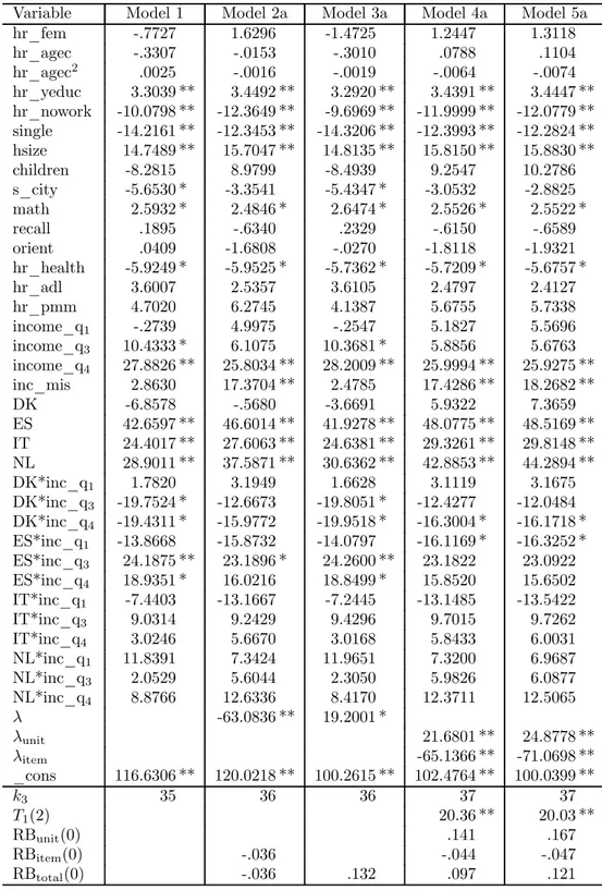
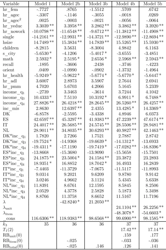
We estimate five alternative models. Model 1 is a standard linear model estimated for the fully responding units without accounting for selectivity generated by nonresponse. Model 2a is a clas-sical sample selection model estimated for the unit respondents and only accounts for selectivity generated by item nonresponse. Model 3a is a classical sample selection model estimated for the

1 1 _{Extensive discussions on the definition of household income, item response rates, unfolding-bracket questions,}

and imputation procedures adopted in SHARE are given in Börsch-Supan and Jürges (2005).

1 2 _{Estimates of a regression model reveals that this module tends to last longer for interviewers with higher age}

full sample with a single indicator (D = Y1Y2) for unit and item response. Model 4a is a generalized

sample selection model which accounts for selectivity generated by unit and item nonresponse, but assumes that errors in the unit and the item response equations are independent. Finaly, Model 5a is a generalized sample selection model which accounts for selectivity generated by unit and item nonresponse, and does not impose independence of the error terms in the two response equations. To control for possible effects due to “mismatch” between the interviewer and the interviewee, we also present the results obtained by introducing interaction terms in the age, gender and schooling level of the interviewer and the interviewee (Models 2b, 3b, 4b, and 5b). Parametric estimates of these models are provided in Tables 6—13.

All estimated models share two common features. First, given the high comparability of the SHARE data, we pool data from the various countries and introduce country indicators plus their interactions with income quartiles to capture unobserved heterogeneity across countries. Pooling the data allows us to increase efficiency of estimation and helps reducing problems of collinear-ity due to the limited within-country variabilcollinear-ity of some variables (like the characteristics of the

fieldwork and the interviewers).13 Second, identifiability of the model parameters is achieved by

imposing a common set of exclusion restrictions. As mentioned in Section 2.1, our exclusion restric-tions are based on characteristics of the fieldwork, the interview process and the interviewers. In particular, characteristics of the fieldwork are used to predict unit nonresponse, characteristics of the interview process are used to predict item nonresponse, and socio-demographic characteristics of the interviewers are used to predict both. Thus, if we distinguish between sampling frame or fieldwork information (Z), characteristics of the household or the HR (V ), characteristics of the interviewer or the interview process (W ), and country dummies (D), then the sets of predictors in each of the three model equations are

X1= (Z, W, D),

X2= (V, W, W∗, D),

X3= (V, D).

where W∗ are characteristics of the interviewer or interview process which are only relevant for the

item response equation. The use of this large set of exclusion restrictions should protect against problems of collinearity, especially in the second estimation step.

Estimates of the response probability for Model 3 are presented in Table 6, while estimates of the probability of participation for Models 4 and 5 are presented in Table 7. After dropping

1 3

a few cases with missing data on the covariates, the sample size consists of 12,537 households, of which 6,746 (53.8 percent) participated to the survey. The reference category for the unit response equations is always a Swedish male aged 55, who received 4 call attempts during fieldwork lasting one month, and was approached by a male interviewer of the same age and schooling level.

Other things being equal, we find that the relationship between the probability of participation and the age of the sampled household member has an inverted-U shape, with a maximum at 62 years of age. Women are less likely to participate than men, but the differences are not strongly significant. The interviewer’s gender does not seem to matter, whereas the interviewer’s age is positively related to unit response. The interviewer’s education, the total number of calls and the length of the fieldwork are negatively related to unit response. These negative relations may simply reflect the strategy of increasing the number of calls (specially those in the evening) and switching to more experienced interviewers when there are difficulties in reaching contact and gaining respondents’ cooperation. As for the interaction between characteristics of the interviewee and the interviewer, we find that the age interactions are significant at the 1 percent level, while the gender interaction is not. While the AIC tends to select the less parsimonious models with interactions, the BIC tends to select the more parsimonious ones without interactions.

Estimates of the probability of item response for food expenditure at home and total nondurable expenditure are presented in Tables 8 and 9 respectively. The reference category for the item response equations is now a Swedish male worker aged 55, with 13 years of education, living in a couple without children, residing in a big city, with good cognitive abilities and health conditions, in the second income quartile, with income not missing, interviewed by a male interviewer of the same age and schooling level, and with the interview conducted at the respondent home, without proxy, and lasting one hour.

Other thing being equal, we find that the probability of item response tends to fall with the age of the HR and with the presence of children aged less than 6 years. Living in a small city, being employed, being single, or being more educated are negatively related to item response, but the es-timated effects are only weakly statistically significant. Even after controlling for the respondent’s background characteristics (like age and education), the scores obtained on the cognitive ability tests are positively related to item response, while other health measures are not. The positive and significant coefficients on the third and forth income quartiles suggest that item nonresponse may lead to selection of households with higher income. Furthermore, the negative coefficient on the dummy for income imputations suggests that nonresponse to income questions is positively

related to nonresponse to consumption expenditure questions. Among characteristics of the inter-view process and the interinter-viewers, we find that allowing the interinter-viewee to be assisted by a proxy respondent, conducting the interview at the respondent home, and using more experienced inter-viewers (that is, interinter-viewers with better computer skill) are positively related to item response. Interaction terms do not seem to be important predictors of the probability of item response. For food consumption at home, both AIC and BIC tend to select models without interactions. For total nondurable consumption, AIC tends to select models with interactions, while BIC tends to select

models without interactions.14 Estimates of the correlation coefficient ρ12 are very close to zero,

and the corresponding likelihood ratio tests never reject conditional independence between unit and item nonresponse. Accordingly, the differences between the estimated coefficients of the probit model (Models 4a and 4b) and the bivariate probit model (Models 5a and 5b) are not statistically significant.

Finally, Tables 10—13 present estimates of the Engel curves for food expenditure at home and total nondurable expenditure. For both consumption expenditure items, the selection biases asso-ciated to unit and item nonresponse have opposite sign and therefore partly offset each other: the first (unit nonresponse) is positive, the second (item nonresponse) is negative.

Estimates of the model parameters can be used to estimate the relative total nonresponse bias for the reference category (corresponding to X = x)

RBtotal(x) =

E(U3| U1> −μ1(x), U2> −μ2(x))

μ3(x)

,

where μj(x) = αj+ βj>x, j = 1, 2, 3. For our parametric model, this is just the sum of the relative

biases due to unit and item nonresponse. The relative unit nonresponse bias for the refence category ranges between 8 percent and 10 percent for food expenditure at home, and between 14 percent and 18 percent for total nondurable expenditure. The relative item nonresponse bias ranges instead between -2 percent and -3 percent for food expenditure at home, and between -3 percent and -5 percent for total nondurable expenditure. For food expenditure at home, the coefficients on the bias

correction terms λunit and λitem are not statistically significant, and estimates of the five models

are not very different. We conclude that unit and item nonresponse appear to be purely random. For total nondurable expenditure, the coefficients on the bias correction terms are statistically significant at the 1 percent level. Therefore, neither unit nor item nonresponse errors are ignorable, and only estimates of Models 4 and 5 are consistent.

1 4

As mentioned in Section 2.2, the assumption of Gaussian errors is critical for our parametric estimates of sample selection models. Parametric estimators are indeed inconsistent if this distri-butional assumption is not valid. Conditional moment tests provide a simple way of testing for

this assumption.15 Because errors of the unit and the item response equations are independent

under the null hypothesis (see Tables 8 and 9), tests for Gaussianity can be conducted separately by testing for Gaussianity in two simple probit models. Following Pagan and Vella (1989), these conditional moment tests can be computed via artificial regressions in which the sample third and forth moments are regressed against an intercept and the score obtained from the probit model. Under the null, the coefficients on the intercepts should be equal to zero. Thus, a test for the joint significance of these coefficients is a test for Gaussianity in the probit model. The independence of the error terms in the two response equations is also useful to test Gaussianity in the outcome equation. In this case, a straightforward generalization of the RESET-like test proposed by Pagan and Vella (1989) consists of augmenting the second estimation step with the additional variables ζU j = ˆμj1λˆ1, ζIj = ˆμj2λˆ2 and ζrs = ζU rζIs (with j = 1, 2, 3 and r, s = 0, 1, 2, 3), and then testing

their joint significance.16 Tables 14 and 15 focus on Model 5a and provide tests for the assumption

of Gaussian errors in the two response equations and in the outcome equation respectively. Overall, our results suggest that the Gaussian assumption is strongly rejected for the unit response equation, but not for the other two equations. As a consequence, parametric estimators may be inconsistent.

4.2

Semiparametric estimates

In this section, we focus on Model 5a and presents estimates of the semiparametric two-step pro-cedure that are robust to departures from the assumption of Gaussian errors.

In the first step of the procedure, parameters of the unit and item response equations are esti-mated jointly by the SNP estimator discussed in Section ?? for two choices of K (the degree of the Hermite polynomial used for approximating the bivariate density of the error terms), namely K = 3 and K = 4. The model specifications underlying these different choices are then compared through a likelihood ratio test, AIC, and BIC. For all model selection criteria, the preferred specification has K = 3 for both food expenditure at home and total nondurable expenditure. Parametric and SNP estimates of these models are presented in Tables 16—19. Notice that, because of the different scale, estimated coefficients of the SNP model and the bivariate probit model with sample selec-tion are not directly comparable. Thus we compare ratios of the estimated coefficients, obtained

1 5 _{For an extensive discussion of conditional moment tests see Newey (1985) and Pagan and Vella (1989).} 1 6 _{Here, ˆλ}

after dividing by the absolute value of the coefficient for the length of the fieldwork (lfield) in the unit response equation and the basolute value of the coefficient on the length of the IV module (ivlength) in the item response equation (and then dividing again by 100). The standard errors of these normalized coefficients are computed using the delta method.

For the unit response equation, we find significant differences between the SNP and the paramet-ric estimates. The main differences occur for interviewers’ characteristics, features of the fieldwork, and country dummies. The assumption of Gaussian error in the unit response equation is again

rejected at the 1 percent level by a Wald test on the joint significance of the γ1h parameters in

the approximation (13). The semiparametric estimate of the marginal density function exhibits positive skewness and lower kurtosis than a standard normal density. Furthermore, the density plot in Figure 1 also reveals the presence of multiple modes.

For the item response equation, we find that Gaussianity is still rejected for food expenditure at home but not for total nondurable expenditure. The marginal densities underlying the two item response equations appear to have a similar shape. They are both platikurtic, exhibit negative skewness, and have a secondary mode in the lower tail of the distribution (see Figure 1). For the item response equation, however, departures from the assumption of Gaussian errors appear to be less harmful. Once the different scale in taken into account, the differences between the parametric and the SNP estimates in Table 19 are small.

In the second step of the procedure, estimates of the two indexes ˆμ1and ˆμ2 are used to estimate

a partially linear model for the outcome variables of interest. Following Robinson (1988), the unknown conditional expectations in (15) are estimated nonparametrically by Nadaraya-Watson bivariate kernel regression estimators, where the bivariate kernel is the product of two univariate

bias reducing kernels with the same bandwidth hn = O(n−1/p). In computing the nonparametric

estimates, we also trim observations for which the denominator of the Nadaraya-Watson estimator

is smaller than a threshold bn= O(n−1/r). In the application, we experiment with different values

of p and r. After replacing the unknown conditional expectations in (15) with their nonparametric

estimates, the vector β3 of slope parameters is estimated by standard OLS with no intercept.17

Standard errors of the OLS estimator are instead computed by the nonparametric bootstrap with 50 replications.

Semiparametric estimates of the partially linear model for food expenditure at home and total nondurable expenditure are presented in Tables 20 and 21 respectively. To explore sensitiveness of

1 7

As mentioned in Section 2.2, the intercept coefficient is absorbed in the nonlinear function g and is not separately identified.

Robinson’s estimator with respect to choice of the bandwidth parameter hn and the threshold bn,

estimation is carried out for various alternative combinations of p and r.18 _{In particular, results}

are presented for p = 5 and r = 21 (Model A), p = 6 and r = 13 (Model B), p = 7 and r = 10 (Model C). Parametric estimates are also reported to facilitate comparisons.

According to our estimates, the Robinson’s estimator is not very sensitive to the choice of the

bandwidth hn and the threshold bn. The only exception is Model A in Table 20. For this model,

the low value of the bandwidth and the high value of threshold lead to imprecise estimates. For food expenditure at home, we find that the estimated coefficients of the partially linear are very close to their parametric counterparts. This suggests that parametric estimates are only marginally affected by departures from Gaussianity. For total nondurable expenditure, instead, the differences between the parametric and the semiparametric estimates are somewhat larger, especially for the coefficients on the income quartiles and their interactions with the country dummies.

5

Conclusions

In this paper we investigate problems of selectivity generated by unit and item nonresponse in cross-sectional surveys, or equivalently, in the first wave of a panel survey.

We first analyze a general sample selection model in which unit and item nonresponse can si-multaneously affect a regression relationship of interest through NMAR missing data mechanisms. Issues concerning identification and estimation have been considered for two alternative specifica-tions of this model. In the parametric specification, errors in the two selection equaspecifica-tions and in the equation for the outcome of interest are assumed to follow a trivariate Gaussian distribution, and model parameters are estimated by the parametric two-step procedure proposed by Poirier (1980). In the semiparametric specification, error terms are assumed to follow an unknown distribution, and model parameters are estimated by a semiparametric two-step procedure which involves a gen-eralization of the SNP estimator proposed by Gallant and Nychka (1987) in the first step, and the semiparametric estimator of Robinson (1988) in the second step.

We then use data from the first wave of SHARE to investigate whether selectivity associated with unit and item nonresponse may bias the estimation of Engel curve for food expenditure at home and total nondurable expenditure. Overall, the amount of bias generated by unit and item nonresponse does not seem to be ignorable. According to our estimates, the relative unit nonresponse bias for

1 8 _{Combinations of p and r are selected to satisfy conditions imposed on the choice of the bandwidth parameter}

the refence category ranges between 8 percent and 10 percent for food expenditure at home, and between 14 percent and 18 percent for total nondurable expenditure. The relative item nonresponse bias ranges instead between -2 percent and -3 percent for food expenditure at home, and between -3 percent and -5 percent for total nondurable expenditure. According to several specifications of our sample selection models, unit and item nonresponse errors appear to be purely random for food expenditure at home, whereas they are not ignorable for total nondurable expenditure.

Diagnostic tests based on the conditional moment framework of Pagan and Vella (1989) and on the SNP framework do not support the assumption of Gaussian errors, specially in the unit response equation. Nevertheless, estimates of our semiparametric two-step procedure do not lead to very qualitative different results.

References

Battistin E., R. Miniaci, and G. Weber (2003), “What Do We Learn from Recall Consumption Data?”, Journal of Human Resources, 38: 354—385.

Börsch-Supan A., A. Brugiavini, H. Jürges, J. Mackenbach, J. Siegrist and G. Weber (2005), Health, Ageing and Retirement in Europe - First Results from the Survey of Health, Ageing and Retirement in Europe, MEA, Mannheim.

Börsch-Supan A., and H. Jürges (2005), The Survey of Health, Ageing and Retirement in Europe - Method-ology, MEA, Mannheim.

Browning M., T.F. Crossley, and G. Weber (2002), “Asking Consumption Questions in General Purpose Survey”, Economic Journal, 113: 540—567.

Das M., W.K. Newey, and F. Vella (2003), “Nonoparametric Estimation of Sample Selection Models”, Review of Economic Studies, 70, 33—58.

Eurostat (1997), “Response rates for the first three waves of the ECHP”, PAN 92/97, Luxembourg. Fitzgerald J., P. Gottschalk, and R. Moffitt (1998), “An Analysis of Sample Attrition in Panel Data: The

Michigan Panel Study of Income Dynamics”, Journal of Human Resources, 33: 251—299.

Gabler S., F. Laisney, and M. Lechner (1993), “Semiparametric Estimation of Binary-Choice Models with an Application to Labor-Force Participation”, Journal of Business and Economic Statistics, 11: 61—80. Gallant A.R., and D.W. Nychka (1987), “Semi-Nonparametric Maximum Likelihood Estimation”,

Econo-metrica, 55: 363—390.

Gerfin M. (1996), “Parametric and Semi-Parametric Estimation of Binary Response Model of Labor Market Participation”, Journal of Applied Econometrics, 11: 321—339.

Groves R.M., and M.P. Couper (1998), Nonresponse in Household Interview Surveys, Wiley, New York. Groves R.M., D.A. Dillman, J.L. Eltinge, and R.J.A. Little (2002), Survey Nonresponse, Wiley, New York. Ham J.C. (1982), “Estimation of a Labour Supply Model with Censoring due to Unemployment and

Underemployment”, Review of Economic Studies, 49: 335—354.

Heckman J. (1979), “Sample Selection Bias as a Specification Error”, Econometrica, 47: 153—161.

Horowitz J., and C.F. Manski (1998), “Censoring of Outcomes and Regressors due to Survey Nonresponse: Identification and Estimation using Weights and Imputations”, Journal of Econometrics, 84: 37—58. Ichimura H., and L.F. Lee (1991), “Semiparametric Least Square of Multiple Index Models: Single Equation

Estimation”, in W.A. Barnett, J. Powell, and G. Tauchen (eds.), Nonparametric and Semiparametric Methods in Econometrics and Statistics, Cambridge University Press, Cambridge.

Klein R., and R. Spady (1993),“An Efficient Semiparametric Estimator for the Binary Response Model”, Econometrica, 61: 387—421.

Lee L.F. (1995), “Semiparametric Maximum Likelihood Estimation of Polychotomous and Sequential Choice Models”, Journal of Econometrics, 65: 381—428.

Lessler J.T., and W.D. Kalsbeek (1992), Nonresponse Errors in Surveys, Wiley, New York.

Leung S.F., and S. Yu (1996), “On the Choice between Sample Selection and Two-Part Models”, Journal of Econometrics, 72: 197—229.

Little R.J.A., and D.B. Rubin (2002), Statistical Analysis with Missing Data (2nd ed.), Wiley, New York. Manski C.F. (2003), Partial Identification of Probability Distribution, Springer, New York.

Melenberg B., and A. van Soest (1996), “Measuring the Costs of Children: Parametric and Semiparametric Estimators”, Statistica Neerlandica, 50: 171—192.

Nicoletti C., and F. Peracchi (2005), “Survey Response and Survey Characteristics: Microlevel Evidence from the European Community Household Panel”, Journal of the Royal Statistical Society, Series A, 168: 763—81.

Newey W. (1985), “Maximum Likelihood Specification Testing and Conditional Moment Tests”, Econo-metrica, 53: 1047—1070.

Newey W. (1999), “Two Step Series Estimation of Sample Selection Models”, unpublished.

O’Muircheartaigh C., and P. Campanelli (1999), “A Multilevel Exploration of the Role of Interviewers in Survey Nonresponse”, Journal of the Royal Statistical Society, Series A, 162: 437—446.

Pagan A., and F. Vella (1989), “Diagnostic Test for Models Based on Individual Data: A Survey”, Journal of Applied Econometrics, 4: 29—59.

Poirier D. (1980), “Partial Observability in Bivariate Probit Models”, Journal of Econometrics, 12: 209— 217.

Puhani P. A. (2000), “The Heckman Correction for Sample Selection and its Critique”, Journal of Economic Surveys, 14: 53—68.

Riphahn R. T., and O. Serfling (2002), “Item Nonresponse on Income and Wealth Questions”, Discussion Paper No. 573, IZA Bonn.

Robinson P.M. (1988), “Root-N-Consistent Semiparametric Regression”, Econometrica, 56: 931—954. Rubin D.B. (1976), “Inference and Missing Data”, Biometrika, 63: 581—592.

Stewart M.B. (2004), “Semi-Nonparametric Estimation of Extended Ordered Probit Models”, The Stata Journal, 4: 27—39.

Vella F. (1998), “Estimating Models with Sample Selection Bias: A Survey”, Journal of Human Resources, 33: 127—169.

Winter J. (2004), “Response Bias in Survey-Based Measures of Household Consumption”, Economics Bul-letin, 3: 1—12.

Table 1: Unweighted household response rates.

Response Noncontact Refusal Other noninterview

Country Eligible rate rate rate rate

Denmark 1742 .61 .09 .29 .01 Italy 2505 .54 .08 .36 .02 Netherlands 2509 .62 .05 .32 .01 Spain 2619 .50 .13 .36 .01 Sweden 3956 .47 .06 .42 .05 Total 13331 .55 .08 .35 .02

Table 2: Unweighted item response rates for consumption expenditure questions.

Food Nondurable

Country Eligible at home consumption

Denmark 1178 .81 .79 Italy 1376 .85 .84 Netherlands 1559 .89 .77 Spain 1341 .78 .77 Sweden 1850 .93 .90 Total 7304 .85 .81

Table 3: Summary statistics for consumption expenditure questions. Yearly amounts expressed in 100 Euro. Empirical distributions trimmed symmetrically by 2 percent.

Variable Obs. Mean Std. Min Max

Food at home 6067 49.6 42.4 .9 640

Nondurable consumption 5780 118.0 86.9 11.7 1280

Table 4: Summary statistics for the fraction of imputed household income by missing income components.

Missing Fraction of imputed income

components Eligible Mean P25 P50 P75

0 3411 1 1943 .20 .00 .02 .29 2 1091 .47 .07 .42 .88 3 527 .59 .18 .68 1.00 4 or more 332 .72 .47 .88 1.00 Total 7304 .37 .01 .20 .76