simulations in Augmented Reality
Lorenzo Mariti, Pier Paolo Valentini1
Abstract. In this chapter, an enhanced methodology for interactive, accurate, fast and robust multibody simulations using Augmented Reality is presented and dis-cussed. This methodology is based on the integration of a mechanical tracker and a dedicated impulse based solver. The use of the mechanical tracker for the inter-action between the user and the simulation allows to separate the processing of the data coming from the position tracking from those coming from the image colli-mation processing. By this way simulation results and visualization remain sepa-rated and the precision is enhanced. The use of a dedicated sequential impulse solver allows a quick and stable simulation also for a large number of bodies and overabundant constraints. The final result of this work is a software tool able to manage real time dynamic simulations and update the augmented scene according-ly. The robustness and the reliability of the system will be checked over two test cases: a ten pendula dynamic system and of a cross-lift mechanism simulation.
Keywords: Augmented Reality, Interactive Multibody Simulation, User Track-ing, Sequential Impulse Solver.
1. Introduction
During the last years, many investigations focused on the increasing trend of using Augmented Reality (AR) [1] to support a variety of engineering activities and to develop interactive tools in design. Augmented Reality has been used for support-ing geometrical modelsupport-ing [2], reverse engineersupport-ing [3], assembly simulation [4-7], analysis [8].
The augmented reality deals with the combination of real world images and computer generated data. Most AR research is concerned with the use of live vid-eo imagery which is digitally processed and augmented by the addition of com-puter generated graphics. The purpose of the augmented environment is to extend
1Pier Paolo Valentini, corresponding author.
Department of Industrial Engineering, University of Rome “Tor Vergata”, via del Politecnico, 1, 00133, Rome, Italy. E-mail: [email protected]
the visual perception of the world, being supported by additional information and virtual objects. One of the most important feature of AR is the possibility to em-bed an high level of user's interaction with the augmented scene [9].
Some recent contributions showed an increasing interest in developing environ-ments for simulating and reviewing physical simulations based on Augmented Re-ality [10-14]. They focused on the interactivity between the user and the augment-ed environment. By this way, the user is not a mere spectator of the contents of the augmented scene, but influences them. Interaction in dynamic simulations can concern both the definition of boundary conditions and initial parameters and the real time control of the process.
In a recent paper [15], P.P. Valentini and E. Pezzuti developed a methodology for implementing, solving and reviewing multibody simulation using augmented reality. According to their results, augmented reality facilitates the interaction be-tween the user and the simulated system and allows a more appealing visualization of simulation results. For this reason, this approach has revealed to be suitable for didactical applications and teaching purposes as well.
On the other hand, the development of multibody simulations in augmented real-ity requires very fast solver in order to produce a smooth animation and an effec-tive illusion. Valentini and Pezzuti proposed to use an optical marker to track the position of the user and interact with the objects in the scene. Moreover, they de-veloped some simple examples to introduce the methodology.
Starting from the discussed background, this chapter aims to discuss two im-portant enhancements of the work in [15] in order to improve the accuracy of us-er's interaction and to allow a robust simulation of large multibody systems. The accuracy in tracking the user is important to perform precise simulation that are required in many engineering applications. The use of optical marker is simple but in this case position tracking error highly depends on the resolution of the camera sensor and on the distance between the camera and the marker. Using standard USB cameras, this error can be some millimeters and can be inacceptable for pre-cise applications, and unwanted flickering may occur due to the tracking algorithm limitations [16]. In order to improve the accuracy in tracking, in the present study we have included the use of a mechanical instrumented arm which is able to achieve a precision of about 0.2 mm in a working space of about 1.2 m of diame-ter. This enhancement is also important to separate the processing of the data com-ing from the position trackcom-ing from those comcom-ing from the image processcom-ing (for perspective collimation and visualization issues). By this way, higher precision in the analysis results can be achieved and only the graphical visualization is affected by optical imprecision.
The second enhancement which has been proposed and tested, is about the use of a dedicated solver for managing the integration of the equations of motion. The implemented solver makes use of the sequential impulse strategy [17] which al-lows a quick and stable simulation also for a large number of bodies, in presence of overabundant and unilateral constraints. According to some authors and
appli-cations (i.e. [18-19]), this approach leads to a very fast and stable solution, but quite less accurate than global solution methods.
The chapter is organized as follows. First of all, a brief introduction about the state of the art of virtual engineering in augmented reality is presented, focusing on the aspects related to multibody simulations. Then, a description of hardware and software implementations is discussed, including the explanation of the itera-tive impulse solver and the details about the strategy for implementing interaction between the user and the scene. In the second part, two examples are presented and discussed.
2. Multibody simulations in Augmented Reality environments
The first and basic implementation of multibody simulations in augmented reality is about the possibility to project on a real scenario the results coming from a pre-computed simulation. It concerns the rendering on the augmented scene of all the objects involved in the simulation whose position is updated according to the re-sults of the simulation.
This implementation is similar to that of the common post-processing software for visualizing graphics results. The only difference is in the introduction of the simulated system in a real context. The advantage is to perceive the interaction with the real world and check working spaces, possible interferences, etc.
Although it can be useful, this approach does not unveil all the potential of AR [15]. A more powerful way to enhance multibody simulation is to introduce an high level of interactivity. It means that the user does not only watch the augment-ed scene, but interacts with it. In this case, the solution of the equations of motion has to be computed synchronously to the animation in order to populate the scene with quickly updated information.
With this type of interaction, the user is active in the scene and can change the augmented contents by picking, pushing and moving objects and controlling the provided information and the environment behaves according to realistic physics laws. The interaction is carried out with advanced input/output devices involving different sensorial channels (sight, hear, touch, etc.) in an integrated way [20]. In particular, in order to interacts with digital information through the physical envi-ronment, the environment has to be provided of the so called Tangible User Inter-faces (TUIs) [21-23].
In the most simple implementations, the patterned markers used for collimating real and virtual contents are used also as TUIs. In advanced implementation visual interaction is achieved by dedicated interfaces (mechanical, magnetic, optical, etc.). By this way, the image processing for the computation of the camera-world perspective transformation can be separated from the acquisition and processing of the user intent. Thanks to this split computation, it is possible to achieve a very precise interaction and simulation and a less precise (and more efficient) visual collimation. This means that the results of the simulations can be accurate and
suitable for technical and engineering purposes. On the other hand, the small im-precisions in the optical collimation are limited to graphics display.
Starting from these considerations, the generic integration algorithm between multibody simulations and augmented reality presented in [15] can be modified separating the contributions of interaction and collimation. For this reason, an high-interactive generic multibody simulation in augmented reality can be imple-mented following five main steps:
1. Before the simulation starts, the geometries and topological properties (joints and connections) have to be defined (as for any multibody sys-tem);
2. The real scene has to contain information for collimating the real world to the virtual objects;
3. The real environment has to contain one or more TUIs for the acquisition of the user’s intent of interacting with the scene;
4. During each frame acquisition, the user’s intent has to be interpreted; the multibody equations have to be built and solved synchronously in order to compute the correct position of all the virtual bodies in the scene; 5. For each frame acquisition, virtual objects have to be rendered on the
scene, after the numerical integration, in the correct position and atti-tude.
3. Implementation of the Augmented Reality environment
3.1 Hardware setup
For the specific purpose of this investigation, the implemented AR system (depict-ed in Figure 1) includes an input video device Microsoft LifeCam VX6000 USB 2.0 camera, an Head Mounted Display (Emagin Z800) equipped with OLed dis-plays, a Revware Microscribe GX2 mechanical tracker and a personal computer.
The Revware Microscribe is an instrumented arm (digitizer) which can be grabbed and driven by the user and possesses five degrees of freedom. It is able to acquire the real-time position of its tip stylus. The operating space is a sphere of about 1.2 m of diameter and the precision of tracking is up to 0.2 mm.
3.2 Implementation and interaction strategy
In order to implement a AR environment suitable for multibody dynamics interac-tive simulation, we have chosen the following strategy (see Figure 2). Before the simulation starts, the geometries and topological properties (joints and
connec-tions) h has to c Usually nized by tation of Fig. 1. A During quired a puting t preted a with the pute the the user After the corr All th guage a processi have to be def contain inform y this operatio y the processi f the camera p ugmented reali g each frame as well. This t the position an and transferred e scene). Then e correct posit r's intent. this computat rect position an e supporting s and Microsoft ing have bee
fined (as for a mation for co n is performe ing units. For point of view a ity hardware se acquisition, th task can be pe nd attitude of d as a spatial n, the multibo tion of all the
tion, al the vir nd attitude. software has b t Visual Stud en developed any multibody ollimating the ed by a pattern the scope it i and the corres
etup
he position of erformed usin f its end effec input for the dy equations virtual bodie rtual objects h been impleme dio 2003 deve using the o y simulation). real world to ned planar ma s necessary to sponding pers f the user in th g the mechan tor. This info simulation (us have to be so es in the scene have to be ren ented using C+ eloping suite. open source l
Then, the rea o the virtual arker which is o perform the pective effect he scene has to ical tracker an rmation can b ser's intent to lved in order e, taking into dered on the s ++ programm Routines for libraries name al scene objects. s recog- compu-t. to be ac-nd com-be inter-interact to com-account scene in ming lan-r image med
AR-Toolkit librarie ognize techniq tween m tion is and rea of the l Fig. 2. M The M that all mented the five stylus t 2 The http://sou 3 http:// t2 which has b es comprise a planar pattern ques, the routi
markers and c necessary for al scene. The library can be Multibody simu Microscribe G ows the real t d arm. This lib e revolute joi tip by solving ARToolkit l urceforge.net/pr /www.hitl.washi been successf set of numeri ned markers i ines are also a camera with go r an accurate details about found on the ulation in augme GX2 has been time access to brary interpret ints of the me an open kinem ibraries can roject/showfiles. ington.edu/artoo fully used in ical procedure in a video stre able to compu ood precision perspective c specific impl internet site o ented reality pr n integrated u o position and ts the output c echanical arm matic chain pr n be freely .php?group_id=1 olkit/ many previou es which are a eam in real ti ute relative po n for visual pu collimation be lementation a of the develop rocedural schem
using the Mic d attitude of e coming from t m and comput roblem. downloaded f 116280 us investigatio able to detect me. Using co sition and atti rposes. This c etween virtual and about the
ers3. me. croscribe SDK ach link of th the rotation se es the positio
from the inte
ons. The and rec-orrelation itude be- computa-l entities contents K library he instru-ensors of on of the ernet site
For m renderin using O Detail the syste All th ronment
3.3 Co
The firs mation the digi by an im scene an era and augmen Fig. 3. C 4 The lib managing comp ng tasks about OpenGL library ls about the pr em under inve ese pieces of t.ollimation P
st step in the i between the i tal camera. T mage processi nd to compute the real word nted scene in thollimation betw
brary can be free
plex geometri t virtual objec y. rocedures for d estigation hav software hav
Procedure
integration of information a he video strea ing routine. It e the correspo d. This matrix he correct pos ween optical ma ely downloaded es the OpenV cts in the augm deducing and ve been provid ve been integr f the tracker in acquired by th am acquired b t is able to re onding transfo x is used to pr sition and persarker and mech
from the interne
Vrml library4 h
mented scene
solving the eq ded in the next rated into a sin
n the augment he instrumente by the digital ecognize a pat ormation matr roject all the v
spective.
hanical tracking
et site http://open
has been includ have been per
quations of m t sections. ngle simulatio ted scene is th ed device and camera is ela tterned marke rix between th virtual content g system. nvrml.org/ ded. All rformed motion of on envi-he colli-d that of aborated er in the he cam-ts in the
The information acquired by the digitizer is concerned with the position and atti-tude of the end effector with respect to the reference frame fixed to the device it-self.
In order to ensure the collimation between the data stream coming from the camera and that from the tracker, it is important to compute the relative transfor-mation matrix between the tracker and the world (described by the marker). This calibration has to be performed only at the beginning of the application and it has to be repeated only if the relative position between the world marker and the digi-tizer changes.
The calibration procedure can be performed by picking with the tracker stylus a set not-aligned points (four no-coplanar points at least) at known positions with respect to the relative frame associated to the marker.
For expressing the coordinate transformation between points, it is useful to deal with homogeneous transformation matrices which include information on both ro-tation and translation parameters. A generic homogeneous transformation matrix can be expressed in the form:
Orientation
3x 3
Position
3x10
0
0
1
T
(1)In the same way, a generic point can be expressed with the following coordinate vector:
P
x
y
z
1
T (2) The coordinate transformation of a generic point P from the local coordinate system fixed to the digitizer to the world coordinate system attached to the marker can be written as:
digitizer
world
world digitizer
P
T
P
(3)where:
P
world is the vector containing the coordinate of the point P expressed in the world reference frame;
P
digitizeris the vector containing the coordinate of the point P expressed in the local (tracker) reference frame.Considering a collection of points
P
1P
2...
P
n, we can built two matrices as:
P
world
P
1 world
P
2 world...
P
n world
(4)
P
digitizer
P
1 digitizer
P
2 digitizer...
P
n digitizer
In order to compute the matrix
T
worddigitizer
we have to solve the following sys-tem of equations:
digitizer
world world digitizerP
T
P
(6) for the unknown elements of the matrix
T
worddigitizer
.An homogeneous transformation matrix is defined by 6 independent parameters (three for the description of the rotation and three for the translation). For this rea-son, the system (6) has more equations than unknowns and the solution can be computed as:
1
T
worlddigitizer
P
worldP
digitizer(7)
where the
1
world
P
is the pseudo-inverse matrix of the
world
P
matrix. Due to numerical approximation or errors in acquisition, the orientation block of the computed matrix
T
worddigitizer
can result not exactly orthogonal. Since it repre-sents a rigid spatial rotation, it is important to correct this imprecision. For this purpose, we can operate a QR decomposition of this orientation block:
1 3x 3 1 3x 3 3x 3
Orientation
digitizerword
R
U
(8)
where (due to the QR algorithm):
R
1 is an orthogonal matrix representing the corrected rotation;
U
1 is a matrix whose upper band contains the errors of approximation and the lower band has only zero elements. In case of a pure rotation (orientation block without errors)
U
1
I
.Finally, in order to compute the transformation matrix between the digitizer and the camera
T
cameradigitizer
, useful to collimate the acquired points to the visualized ones, a matrix multiplication has to be performed:
T
cameradigitizer
T
worddigitizer
T
cameraword
(9)Figure 5 shows some snapshots acquired during a calibration procedure. The reference points are picked using a reference cube of known dimensions (80 mm x 80 mm x 80 mm).
Fig. 4. F
3.4 Us
Once th define t A po betwee the sim namics Math spline c motion
F
e
where: Four snapshotsser’s intera
he position an the methods to ssible solutio en the digitizer mulation [24]. of that point hematically, th control point n:
F
ek
f
taken during caaction
nd the attitude o interact with n is the use o r stylus tip an By this way, that moves ac he use of a fict adds a term to
_ tracke springd
virtual alibration proc e of the tracker h the simulatio of a fictitious nd a point belo if the tip is m ccordingly. titious spring o the external
_ _ _ er tip l body point
cedure. r are correctly on. s spring-damp onging to one moved in the sc between the t force vector
_ f spring vc
d
y recorded, we per element co of the rigid b cene, it affects racker stylus t
F
e in equa _ _ _ tracker tip virtual body poine have to onnected bodies in ts the dy-tip and a uations of
nt (10)
tracke virtuald
digitizer
tracke virtuald
_ f sprink
_ f sprinc
In ord an exter ter has proves t Fig. 5. T simulate4. Imp
Given a and sub followin One o equation
where:
M
i
is
_ _ _ er tip l body point is r tip;
_ _ _ er tip l body point is ng is the stiffn ngis the dampi der to prevent rnal (and not pto be chosen the stability of The implementa d bodies.
plementing
a collection o bjected to a se ng different ap of the most use ns, obtaining a
0
M
q
s the inertia m s the vector co s the distance s the derivativ ness coefficien ing coefficien the dynamics physical) elast very stiff. M f the system a ation of a fictitiothe sequen
fn
body rigid et of external pproaches. ed multibody adifferential-
T q
matrix of the c ontaining all th e between the ve of
d
virtualtracker__ nt of the fictiti nt of the fictitio s of the system tic componen Moreover, the and prevents jious spring for
ntial impuls
bodies, cons forces, the eq dynamics for algebraic syst
F
e
ollection of ri he constraint e e connected c
_ _ _ tip body point wi ous spring; ous spring. m to be affecte nt the value of use of a dam ittering in sim managing the use solver
trained byn
j quation of mo rmulation is b tem: igid bodies; equations; control point th respect to t ed by the pres f the stiffness p mping coeffici mulation. user’s interactio joint kinemati otion can be d ased on the L ( and the time; sence of parame-ient im-on to the ic joints deduced Lagrange (11)
q
,
q
and
q
are the vectors of absolute generalized coordinates, velocities and accelerations, respectively;q
is the Jacobian matrix of the constraint equations (differentiated with re-spect to the generalized coordinates);
is the vector of Lagrange multipliers associated to the constraint equations;
F
e is the vector containing all the elastic and external forces (including the fic-titious spring contribution).In order to reduce the complexity of the solution, the constraint equations are of-ten differentiated two times with respect to time and Eq. (11) is rearranged as:
0
T q e qM
q
F
(12) where
q
2
qt
tt qq
q
q
(13)and the subscripts "q" and "t" denote the differentiation with respect to the gener-alized coordinates and time, respectively.
Both Eq. (11) and Eq. (12) allow to solve for the unknown generalized accelera-tion, velocities and positions taking into account all the constraint equations simul-taneously. Of course, this approach can achieve accurate results with suitable DAE solver. On the other hand, a dynamic system with a lot of constraints in-creases the complexity of the problem and the computational effort to solve it. For this reason, the system in (12) can be rearranged for being suitable for the sequen-tial impulse solution strategy.
There are two main steps in the impulse-based methodology. Firstly, the equa-tions of motion are tentatively solved considering elastic and external forces but neglecting all the kinematic constraints. This produces a solution that is only ap-proximated because the constraint equations are not satisfied. In a second step, a sequence of impulses are applied to each body in the system in order to correct its velocity according to the limitation imposed by the constraint. This second step is iterative. It means that a series of impulse is applied to the bodies until the con-straint equations are fulfilled within a specific tolerance. It is important to under-line that each impulse is applied independent from the others. By this way the constraint equations are not solved globally, but iteratively.
4.1 Solving the equations of motion
Following the approach introduced in the previous section, the sequential impulse formulation can be split into two main steps. The first one is about the solution of the equations of motion in (11) neglecting the constraint equations and constraint forces:
M
q
approx
F
e (14)By this way, Eq. (14) can be solved for
q
approx that represent the vector of approximated generalized accelerations.The values of the corresponding approximated generalized velocities and posi-tions can be computed by linear approximation:
q
approx
h q
approx (15)
q
approx
h q
approx (16)where h is the integration time step. In order to correct the
approx
q
and fulfill the constraint equations, a series of impulses
constraint
P
has to be applied to the bodies. Each impulse is computed imposing the fulfillment of the constraint equations written in terms of generalized coordinates. As well-known from the Newton's law, the application of the impuls-es causimpuls-es a variation of momentum:
M
q
corrected
q
approx
P
constraint (17) where
q
correctedis the vector of generalized velocities after the application of impulses
P
constraint.The corrected velocities can be computed from Eq. (17) as:
1
corrected approx constraint
q
q
M
P
(18)Considering that the impulses are related to the constraint equations, they can be computed as
T
q constraint
P
(19)where
is the vector of Lagrange multipliers associated to the impulses. Since the effect of the impulses is to correct the generalized velocities and fulfill the kinematic constraints, the
corrected
q
has to satisfy the constraint equations written in terms of velocities:
0
d
0
d
t
qq
t
(20)
0
qq
corrected t
(21)Inserting Eq. (19) into Eq. (18) and substituting
q
corrected into Eq. (21) we can obtain:
1
0
T qq
approxM
q t
(22)Eq. (22) can be solved for
obtaining:
1
1 T
q
M
q qq
approx t
(23) Then, the impulses can be computed using Eq. (19) and the corrected values of generalized velocities using Eq. (18).Since the impulses are computed sequentially, the global fulfillment of the con-straint equations cannot be directly achieved. Some iterations are required. The computation of
,
constraint
P
and
corrected
q
can be repeated till a tolerance on the fulfillment of Eq. (21) is reached or for a maximum number of time. Expe-rience [17] shows that four or five iterations are sufficient to achieve an adequate tolerance. Since the constraints are imposed at velocity level, a stabilized formula-tion is required to control the constraints fulfillment at the posiformula-tion level. Details are provided in section 4.3.4.2 Computation of reaction forces
When simulating multibody dynamics, one of the most interesting results for en-gineers is the knowledge of the reaction forces, i.e. the forces exerted by the joints.
Using the sequential impulse formulation, the reaction forces cannot be comput-ed directly but a preliminary computation is requircomput-ed. The problem is that impuls-es are applied sequentially, it means that each joint exerts more than one impulse during each time step and the various impulses have to be recollected.
In order to deduce a methodology for evaluating the reaction forces of the joints we have to introduce the concept of the accumulated impulse. It can be defined as the resultant impulse of each joint produced each time step and it can be computed as the sum of all the impulses exerted by the joint over the iteration.
In the solution of the equations of motion, the joint impulses are evaluated using Eq. (23) and Eq. (19). This computation is performed iteratively in order to reach a set of velocities congruent to kinematic joints. It means that at each iteration a new impulse vector
constraint
The accumulated Lagrange multipliers
of the impulses for each time step can be evaluated as:
iterations
(24)The accumulated impulse
P
tot constraint can be computed using Eq. (19) obtain-ing:
T
tot constraint q
P
(25)The reaction forces
constraint
F
exerted by the joints can be computed using the general relation between forces and impulses:
tot constraint constraintP
F
h
(26)4.3 Stability issues
The use of the sequential impulse strategy is subjected to the use of constraint equations expressed in terms of generalized velocity. It means that the exact in-formation about the kinematic joints may be lost during the integration process. In this case a position drift can be observed and stability problems may occur.
In order to enforce the constraints on position a stabilized formulation can be adopted. In this case, the constraint equations in Eq. (21) can be modified as:
0
qq
corrected th
(27)where
is a scalar chosen in the range 0 ÷ 1.5. Examples of simulation
In order to test the proposed methodology and both hardware and software inte-gration, in this section two examples of implementation are presented and dis-cussed.
5.1 Ten pendula dynamic system
The first simulated scenario is about a collection of 10 rigid pendula that move under the effect of gravity. All the pendula have the same geometry and inertial properties which have been summarized in Table 1.
Table 1. Geometrical and inertial parameters of the first example.
Parameter Value Pendulum length 50 mm
Pendulum mass 0.1 kg
Pendulum principal moments of inertia [21,21,0.5] kg
mm2The first pendulum is pivoted to a fixed frame by means of a point-to-point 3 d.o.f. joint. The other pendula are sequentially connected by mean of revolute joints (hinges). The user can interact with the scene by connecting a fictitious spring between the tracker stylus and the free end of the last pendulum. In particu-lar, the user can decide when the connection between the tracker and the last pen-dulum has to be activated (simulating the clipping) or deactivated (simulating the release). This scenario is also important to test the methodology with event based changes in the equations of motion.
In order to achieve stable and correct results, the solution strategy has to be able to manage rapid changes in force definition. The simulation has been performed with a fixed time step of 0.01 s.
Per each video frame, 4 integration steps are computed and the augmented scene is updated accordingly.
Figure 6reports a series of four snapshots taken during the run of the simulation. The rigid body collection is real-time rendered along with the simulation. In the first part of the simulation (snapshot A of Figure 6) the pendula are free to move and they are in an equilibrium position (aligned along the vertical direction).
Then, the user locates the tracker near the last pendulum tip and activates the fic-titious spring connection (snapshot B). From this moment, the tip of the last pen-dulum moves subjected to this connection.
When the user moves the tracker, the tip of the pendulum follows it. It is im-portant to notice that the motion of all the rigid body collection is continuously simulated according to the external action of the gravity and the driving force due to the user’s presence.
When the user decides to release the fictitious spring connection (snapshot C), the collection of pendula moves subjected to gravity force only and it oscillates around the equilibrium position (snapshot D).
Fig. 6.Sn The a the erro system pressed steps w tems (en tribution ing the fictitiou
P
wherePow
tion;
F
fic Eq (10) napshots of the ccuracy and t r in the fulfill (potential, kin using positio hen it reache nergy loss) is n of the extern corresponding us spring and t _ user actioPower
_ user actionwer
_ ctitious spring ; simulation of t the stability o ment of the co netic and elas on variable is s 1.6·10-5 m. below 1%. In nal action of t g power as th the velocity of
on
F
fictitious is the power a is the reactiothe first exampl
of the simulati onstraint equa stic). The nor always lowe The variation n the computa
the user has b he dot product f the digitizer
_ us spring
v
sty associated to on force of th leion have been ations and the rm of the con er than 10-6 m n of the overa tion of the ov been taken into
t between the stylus tip as:
_ tylus tip the reaction f he fictitious sp n checked com overall energ nstraint equati m except for t all energy of t erall energy, t o account by e reaction forc ( force of the us pring compute mputing gy of the ions ex-ten time the sys-the con- evaluat-ce of the (28) ser’s ac-ed as in
v
stylus tip_
is the absolute velocity of the stylus tip.4.2 Cross-lift dynamic simulation
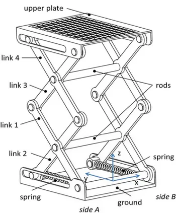
The second simulated scenario is about the dynamic motion of a cross lift device which is comprised of 11 rigid bodies connected by 16 hinges and 4 slider joints (see Figure 7). The links are connected by means of the following constraints: Two revolute joints between the frame and the first link on both side A and B
of the mechanism
Two slider joints between the frame and the second link on both side A and B of the mechanism
Four revolute joints between adjacent links on each side of the mechanism (8 in total)
A revolute joint between the third link and the upper plate on both side A and B of the mechanism;
A slider joint between the fourth link and the upper plate on both side A and B of the mechanism;
Four revolute joints connecting the two horizontal rods between the two side of the mechanism.
Two linear spring-damper elements act horizontally between the frame and the slider joint location of the second link on both side A and B of the mechanism. The gravity field acts downward along the vertical direction.
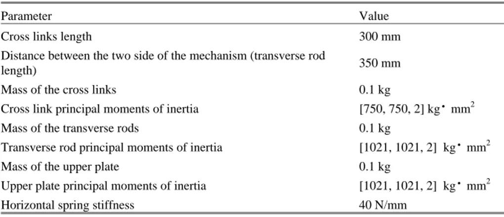
The example has been chosen in order to test the capabilities of the solver to deal with many overabundant constraints. Geometrical, inertial and elastic proper-ties of the simulation have been summarized in Table 2.
Table 2. Geometrical, inertial and elastic parameters of the second example.
Parameter Value
Cross links length 300 mm
Distance between the two side of the mechanism (transverse rod
length) 350 mm
Mass of the cross links 0.1 kg
Cross link principal moments of inertia [750, 750, 2] kg
mm2 Mass of the transverse rods 0.1 kgTransverse rod principal moments of inertia [1021, 1021, 2] kg
mm2Mass of the upper plate 0.1 kg
Upper plate principal moments of inertia [1021, 1021, 2] kg
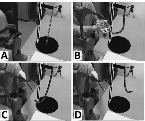
mm2 Horizontal spring stiffness 40 N/mmFig. 7. C The u stylus ti when th (simulat In the fixed tim and the Figure The cro In the to move the mid shot B) the track When tion (sn
ross lift device
ser can intera ip and the mid he connection
ting the clippi same way of me step of 0.0 augmented sc e 8 reports a s ss lift mechan first part of th e and it is in a ddle of the upp . From this m ker and the m n the user mov
apshot C), pre
of the second ex
act with the sc ddle point of th
between the ing) or deactiv f the first exam 01 s. Per each cene is update eries of four s nism is real-tim he simulation an equilibrium per plate and moment, the u echanism mov ves the tracker
eserving the r
xample.
cene by impos the upper plate
tracker and t vated (simulat mple, the sim h video frame ed accordingly snapshots take me rendered a n (snapshot A m position. Th activates the upper plate ve ves subjected r, the upper pl right connectio sing a fictitiou e. In particula the upper plat ting the releas mulation has be
e, 4 integration y.
en during the r along with the of Figure 8) t hen, the user fictitious spri ertical coordin to this connec late follows it on with the ot us spring betw ar, the user can te has to be a
e).
een performed n steps are co
run of the sim simulation. he mechanism locates the tra ng connection nates is contro
ction. t in the vertica ther rigid bodi
ween the n decide activated d with a omputed mulation. m is free acker in n (snap-olled by al direc-dies. It is
importa simulat ing forc When vice m around Fig. 8. S Also checke constra tion (w 10-6 m. increas tems is overall into ac ant to notice t ted according ce due to the u n the user dec oves freely su
the equilibriu
Snapshots of the
for this exam d. Due to the aint equations when the simu
. When the us ses and reache s always below
energy, the c count by eva
that the motio to the externa user’s presenc cides to releas ubjected to gr um position (s e simulation of
mple, the accur presence of a is higher tha lation run wit ser interacts b es 6.1·10-5 m. w 2%. As in t contribution o luating the co on of all the ri al action of th ce. se the fictitiou ravity force an snapshot D).
the second exam
racy and the st a lot of overab an in the prev thout the inter by pushing an
. The variatio the previous e of the externa
orresponding
igid body coll he gravity, the us spring conn nd internal sp mple. tability of the bundant constr ious example raction of the d pulling the n of the over example, in th al action of th power as the ection is cont e springs and nection, the li prings and it o simulation ha raints, the nor
. During the f user) it is low upper plate, t rall energy of he computatio e user has be dot product tinuously the driv-ifting de-oscillates ave been rm of the free mo-wer than the norm f the sys-on of the een taken between
the reaction force of the fictitious spring and the velocity of the digitizer stylus tip using Eq. (28).
6. Conclusions
In this chapter, an enhanced methodology for interactive, accurate, fast and robust multibody simulations of mechanical systems using Augmented Reality has been presented and discussed. This methodology is based on the integration of a me-chanical tracker and a dedicated impulse based solver.
In this context, the simulation of movement of mechanical systems in an Aug-mented Reality environment can be useful for projecting virtual animated contents into a real world. By this way, it is possible to build comprehensive and appealing representations of interactive simulations including pictorial view and accurate numerical results.
In particular, two important enhancements have been presented with respect to a previous implementations. First of all, it has been possible to improve the preci-sion of the interaction between the user and the scene by means of a precise me-chanical tracking instrumentation. This constitutes an important improvement if compared with the use of simple optical markers for tracking the user in the scene. In the latter case, the precision in tracking was affected by the resolution of the camera, while with a mechanical device, it is possible to separate the processing of the data coming from the position tracking, from those coming from the image collimation processing. By this way, the simulation input is independent from the visualization input and output.
The second important enhancement is the use of a dedicated solver based on the sequential impulse strategy in order to perform a fast and robust simulation.
According to this approach, the solution is based on the less computational de-manding solution strategy. Following the implemented algorithm, the equations of motion are firstly tentatively solved considering elastic and external forces but ne-glecting all the kinematic constraints. This produces a solution that is only approx-imated because the constraint equations are not satisfied. In a second step, a se-quence of impulses are applied to each body in the collection in order to correct its velocity according to the limitation imposed by the constraint. This second step is iterative and involves the application of a series of impulses to the bodies until the constraint equations are fulfilled within a specific tolerance.
The final result of this work is a tool able to manage real time dynamic simula-tion and to update the augmented scene accordingly. The robustness and the relia-bility of the system have been checked over two test cases: a ten pendula dynamic system and the dynamics of a cross-lift mechanism.
According to the proposed methodology, the user can directly control the simu-lation by a smooth visualization on the head mounted display.
The integration among Augmented Reality, dedicated solver and precise input tracker can be considered an advantage for the future development of a new class of multibody simulation software. Moreover, this integrated simulation environ-ment can be useful for both didactical purposes and engineering assessenviron-ments of mechanical systems.
References
[1] Azuma R, Baillot Y et al.: Recent advances in augmented reality. IEEE Computer Graphics
21(6), 34–47, (2001)
[2] Gattamelata D, Pezzuti E, Valentini PP: A CAD system in Augmented Reality application,
Proc. of 20th European Modeling and Simulation Symposium, track on Virtual Reality and
Visualization, Briatico (CS), Italy, (2008)
[3] Valentini PP: Augmented Reality and Reverse Engineering tools to support acquisition, pro-cessing and interactive study of archaeological heritage, chapter in Virtual Reality, Nova Pub-lishing, (2011)
[4] Raghavan V, Molineros J, Sharma R: Interactive evaluation of assembly sequences using augmented reality, IEEE Transaction on Robotics and Automation, 15(3), 435-449, (1999) [5] Pang Y, Nee AYC, Ong SK, Yuan ML, Youcef-Toumi K: Assembly Feature Design in an
Augmented Reality Environment, Assembly Automation, 26(1), 34-43, (2006)
[6] Valentini PP: Interactive virtual assembling in augmented reality, International Journal on
Interactive Design and Manufacturing, 3, 109-119, (2009)
[7] Valentini PP: Interactive cable harnessing in Augmented Reality", International Journal on
Interactive Design and Manufacturing, 5(1), (2011)
[8] Gattamelata D, Pezzuti E, Valentini PP: Virtual engineering in augmented reality, chapter in
Computer Animation, Nova Publishing, 57-84, (2010)
[9] Valentini PP, Enhancing user role in augmented reality interactive simulations, chapter in
Human Factors in Augmented Reality Environments, Springer, (2012)
[10] Buchanan P, Seichter H, Billinghurst M, Grasset R: Augmented reality and rigid body simu-lation for edutainment: the interesting mechanism - an AR puzzle to teach Newton physics, Proc. of the International Conference on Advances in Computer Entertainment Technology, Yokohama, Japan, 17-20, (2008)
[11] Chae C, Ko K: Introduction of Physics Simulation in Augmented Reality, Proc. of the 2008
International Symposium on Ubiquitous Virtual Reality, ISUVR. IEEE Computer Society,
Washington, DC, 37-40, (2008)
[12] Kaufmann, H, Meyer, B: Simulating Educational Physical Experiments in Augmented Real-ity, in ACM SIGGRAPH ASIA, (2008)
[13] Irawati S, Hong S, Kim J, Ko H: 3D edutainment environment: learning physics through VR/AR experiences. Proc. of the International Conference on Advances in Computer
Enter-tainment Technology, 21-24, (2008).
[14] Mac Namee B, Beaney D, Dong Q: Motion in augmented reality games: an engine for creat-ing plausible physical interactions in augmented reality games. International Journal of
Computer Games Technology, Article ID 979235, (2010)
[15] Valentini PP, Pezzuti E: Interactive Multibody Simulation in Augmented Reality, Journal of
Theoretical and Applied Mechanics, 48(3), 733-750, (2010)
[16] Azuma RT, Tracking Requirements for Augmented Reality. Communications of the ACM,
vol. 36(7), 50-51, (1993)
[17] Mirtich BV: Impulse-based dynamic simulation of rigid body systems. PhD thesis, Universi-ty of California, Berkeley, (1996)
[18] Schmitt A, Bender J: Impulse-based dynamic simulation of multibody systems: numerical comparison with standard methods. In Proc. Automation of Discrete Production Engineering, 324–329, (2005)
[19] Schmitt A, Bender J, Prautzsch H: On the convergence and correctness of impulse-based dynamic simulation. Internal report, 17, Institut für Betriebs- und Dialogsysteme, (2005) [20] Jaimes A, Sebe N: Multimodal human-computer interaction: A survey. Computer vision and
image understanding, 108(1-2), 116-134, (2007)
[21] Ullmer B, Ishii H: Emerging frameworks for tangible user interfaces. IBM Systems Journal, 39(3-4), 915–931, (2000)
[22] Fiorentino M, Monno G, Uva AE: Tangible Interfaces for Augmented Engineering Data Management. Chapter in Augmented Reality, Intech, Croatia, (2010)
[23] Slay H, Thomas B, Vernik R: Tangible user interaction using augmented reality. Proceed-ings of the 3rd Australasian Conference on User interfaces, Melbourne, Victoria, Australia, (2002)
[24] Valentini PP, Pezzuti E: Dynamic Splines for interactive simulation of elastic beams in Augmented Reality, Proc. of IMPROVE 2011 International Congress, Venice, Italy (2011).
![Fig. 4. F 3.4 Us Once th define t A po betwee the sim namics Math spline c motion F e where: Four snapshots ser’s intera he position an the methods tossible solutioen the digitizermulation [24]](https://thumb-eu.123doks.com/thumbv2/123dokorg/7607288.114917/10.892.199.646.218.659/define-motion-snapshots-position-methods-tossible-solutioen-digitizermulation.webp)