A SEARCH FOR SPECTRAL HYSTERESIS AND ENERGY-DEPENDENT TIME LAGS
FROM X-RAY AND TeV GAMMA-RAY OBSERVATIONS OF Mrk 421
A. U. Abeysekara1, S. Archambault2, A. Archer3, W. Benbow4, R. Bird5, M. Buchovecky5, J. H. Buckley3, V. Bugaev3, J. V Cardenzana6, M. Cerruti4, X. Chen7,8, L. Ciupik9, M. P. Connolly10, W. Cui11,12, J. D. Eisch6, A. Falcone13, Q. Feng2,
J. P. Finley11, H. Fleischhack8, A. Flinders1, L. Fortson14, A. Furniss15, S. Griffin2, N. Håkansson7, D. Hanna2, O. Hervet16, J. Holder17, T. B. Humensky18, M. Hütten8, P. Kaaret19, P. Kar1, M. Kertzman20, D. Kieda1, M. Krause8,
S. Kumar17, M. J. Lang10, G. Maier8, S. McArthur11, A. McCann2, K. Meagher21, P. Moriarty10, R. Mukherjee22, D. Nieto18, S. O’Brien24, R. A. Ong5, A. N. Otte21, N. Park23, V. Pelassa4, M. Pohl7,8, A. Popkow5, E. Pueschel24, K. Ragan2, P. T. Reynolds25, G. T. Richards21, E. Roache4, I. Sadeh8, M. Santander22, G. H. Sembroski11, K. Shahinyan14, D. Staszak23, I. Telezhinsky7,8, J. V. Tucci11, J. Tyler2, S. P. Wakely23, A. Weinstein6, A. Wilhelm7,8, D. A. Williams16
(the VERITAS Collaboration), and
M. L. Ahnen26, S. Ansoldi27,56, L. A. Antonelli28, P. Antoranz29, C. Arcaro30, A. Babic31, B. Banerjee32, P. Bangale33, U. Barres de Almeida33,57, J. A. Barrio34, J. Becerra González35,36,58, W. Bednarek37, E. Bernardini38,39, A. Berti27,59,
B. Biasuzzi27, A. Biland26, O. Blanch40, S. Bonnefoy34, G. Bonnoli29, F. Borracci33, T. Bretz41,60, R. Carosi29, A. Carosi28, A. Chatterjee32, P. Colin33, E. Colombo35,36, J. L. Contreras34, J. Cortina40, S. Covino28, P. Cumani40,
P. Da Vela29, F. Dazzi33, A. De Angelis30, B. De Lotto27, E. de Oña Wilhelmi42, F. Di Pierro28, M. Doert43, A. Domínguez34, D. Dominis Prester31, D. Dorner41, M. Doro30, S. Einecke43, D. Eisenacher Glawion41, D. Elsaesser43,
M. Engelkemeier43, V. Fallah Ramazani44, A. Fernández-Barral40, D. Fidalgo34, M. V. Fonseca34, L. Font45, C. Fruck33, D. Galindo46, R. J. García LÓpez35,36, M. Garczarczyk38, M. Gaug45, P. Giammaria28, N. GodinoviĆ31, D. Gora38, D. Guberman40, D. Hadasch47, A. Hahn33, T. Hassan40, M. Hayashida47, J. Herrera35,36, J. Hose33, D. Hrupec31,
G. Hughes26, W. Idec37, K. Kodani47, Y. Konno47, H. Kubo47, J. Kushida47, D. Lelas31, E. Lindfors44, S. Lombardi28, F. Longo27,59, M. LÓpez34, R. LÓpez-Coto40,61, P. Majumdar32, M. Makariev48, K. Mallot38, G. Maneva48, M. Manganaro35,36, K. Mannheim41, L. Maraschi28, B. Marcote46, M. Mariotti30, M. Martínez40, D. Mazin33,62,
U. Menzel33, R. Mirzoyan33, A. Moralejo40, E. Moretti33, D. Nakajima47, V. Neustroev44, A. Niedzwiecki37, M. Nievas Rosillo34, K. Nilsson44,63, K. Nishijima47, K. Noda33, L. Nogués40, M. Nöthe43, S. Paiano30, J. Palacio40, M. Palatiello27, D. Paneque33, R. Paoletti29, J. M. Paredes46, X. Paredes-Fortuny46, G. Pedaletti38, M. Peresano27, L. Perri28, M. Persic27,64, J. Poutanen44, P. G. Prada Moroni49, E. Prandini30, I. Puljak31, J. R. Garcia33, I. Reichardt30,
W. Rhode43, M. RibÓ46, J. Rico40, T. Saito47, K. Satalecka38, S. Schroeder43, T. Schweizer33, S. N. Shore49, A. Sillanpää44, J. Sitarek37, I. Snidaric31, D. Sobczynska37, A. Stamerra28, M. Strzys33, T. SuriĆ31, L. Takalo44, F. Tavecchio28, P. Temnikov48, T. TerziĆ31, D. Tescaro30, M. Teshima33,62, D. F. Torres50, N. Torres-Albà46, T. Toyama33,
A. Treves27, G. Vanzo35,36, M. Vazquez Acosta35,36, I. Vovk33, J. E. Ward40, M. Will35,36, M. H. Wu42, R. Zanin46,bd (the MAGIC Collaboration),
T. Hovatta51,52, I. de la Calle Perez53, P. S. Smith54, E. Racero53, and M. BalokoviĆ55
1
Department of Physics and Astronomy, University of Utah, Salt Lake City, UT 84112, USA
2
Physics Department, McGill University, Montreal, QC H3A 2T8, Canada
3
Department of Physics, Washington University, St. Louis, MO 63130, USA
4
Fred Lawrence Whipple Observatory, Harvard-Smithsonian Center for Astrophysics, Amado, AZ 85645, USA
5Department of Physics and Astronomy, University of California, Los Angeles, CA 90095, USA 6
Department of Physics and Astronomy, Iowa State University, Ames, IA 50011, USA
7
Institute of Physics and Astronomy, University of Potsdam, D-14476 Potsdam-Golm, Germany
8
DESY, Platanenallee 6, D-15738 Zeuthen, Germany
9
Astronomy Department, Adler Planetarium and Astronomy Museum, Chicago, IL 60605, USA
10
School of Physics, National University of Ireland Galway, University Road, Galway, Ireland
11
Department of Physics and Astronomy, Purdue University, West Lafayette, IN 47907, USA
12
Department of Physics and Center for Astrophysics, Tsinghua University, Beijing 100084, China
13
Department of Astronomy and Astrophysics, 525 Davey Lab, Pennsylvania State University, University Park, PA 16802, USA
14School of Physics and Astronomy, University of Minnesota, Minneapolis, MN 55455, USA 15
Department of Physics, California State University—East Bay, Hayward, CA 94542, USA
16
Santa Cruz Institute for Particle Physics and Department of Physics, University of California, Santa Cruz, CA 95064, USA
17
Department of Physics and Astronomy and the Bartol Research Institute, University of Delaware, Newark, DE 19716, USA
18
Physics Department, Columbia University, New York, NY 10027, USA
19
Department of Physics and Astronomy, University of Iowa, Van Allen Hall, Iowa City, IA 52242, USA
20
Department of Physics and Astronomy, DePauw University, Greencastle, IN 46135-0037, USA
21
School of Physics and Center for Relativistic Astrophysics, Georgia Institute of Technology, 837 State Street NW, Atlanta, GA 30332-0430, USA
22
Department of Physics and Astronomy, Barnard College, Columbia University, NY 10027, USA
23
Enrico Fermi Institute, University of Chicago, Chicago, IL 60637, USA
24
School of Physics, University College Dublin, Belfield, Dublin 4, Ireland
25Department of Physical Sciences, Cork Institute of Technology, Bishopstown, Cork, Ireland 26
ETH Zurich, CH-8093 Zurich, Switzerland
27
Università di Udine, and INFN Trieste, I-33100 Udine, Italy
28
INAF National Institute for Astrophysics, I-00136 Rome, Italy
29
Università di Siena, and INFN Pisa, I-53100 Siena, Italy
30Università di Padova and INFN, I-35131 Padova, Italy 31
Croatian MAGIC Consortium, Rudjer Boskovic Institute, University of Rijeka, University of Split and University of Zagreb, Croatia
32
Saha Institute of Nuclear Physics, 1/AF Bidhannagar, Salt Lake, Sector-1, Kolkata 700064, India
33
Max-Planck-Institut für Physik, D-80805 München, Germany
34
Universidad Complutense, E-28040 Madrid, Spain
35
Inst. de Astrofísica de Canarias, E-38200 La Laguna, Tenerife, Spain
36
Universidad de La Laguna, Dpto. Astrofísica, E-38206 La Laguna, Tenerife, Spain
37
University ofŁódź, PL-90236 Lodz, Poland
38
Deutsches Elektronen-Synchrotron(DESY), D-15738 Zeuthen, Germany
39Humboldt University of Berlin, Institut für Physik Newtonstr. 15, D-12489 Berlin Germany 40
Institut de Fisica d’Altes Energies (IFAE), The Barcelona Institute of Science and Technology, Campus UAB, E-08193 Bellaterra (Barcelona), Spain
41
Universität Würzburg, D-97074 Würzburg, Germany
42
Institute for Space Sciences(CSIC/IEEC), E-08193 Barcelona, Spain
43
Technische Universität Dortmund, D-44221 Dortmund, Germany
44
Finnish MAGIC Consortium, Tuorla Observatory, University of Turku and Astronomy Division, University of Oulu, Finland
45
Unitat de Física de les Radiacions, Departament de Física, and CERES-IEEC, Universitat Autònoma de Barcelona, E-08193 Bellaterra, Spain
46
Universitat de Barcelona, ICC, IEEC-UB, E-08028 Barcelona, Spain
47
Japanese MAGIC Consortium, ICRR, The University of Tokyo, Department of Physics and Hakubi Center, Kyoto University, Tokai University, The University of Tokushima, Japan
48
Inst. for Nucl. Research and Nucl. Energy, BG-1784 Sofia, Bulgaria
49
Università di Pisa, and INFN Pisa, I-56126 Pisa, Italy
50
ICREA and Institute for Space Sciences(CSIC/IEEC), E-08193 Barcelona, Spain
51
Aalto University Metsähovi Radio Observatory, Metsähovintie 114, 02540 Kylmälä, Finland
52
Aalto University Department of Radio Science and Engineering, P.O. BOX 13000, FI-00076 AALTO, Finland
53
European Space Astronomy Centre(INSA-ESAC), European Space Agency (ESA), Satellite Tracking Station, P.O. Box—Apdo 50727, E-28080 Villafranca del Castillo, Madrid, Spain
54
Steward Observatory, University of Arizona, Tucson, AZ 85721, USA
55
Cahill Center for Astronomy & Astrophysics, California Institute of Technology, 1200 E. California Blvd, Pasadena, CA 91125, USA Received 2016 September 26; accepted 2016 November 10; published 2016 December 22
ABSTRACT
Blazars are variable emitters across all wavelengths over a wide range of timescales, from months down to minutes. It is therefore essential to observe blazars simultaneously at different wavelengths, especially in the X-ray and gamma-ray bands, where the broadband spectral energy distributions usually peak. In this work, we report on three “target-of-opportunity” observations of Mrk 421, one of the brightest TeV blazars, triggered by a strong flaring event at TeV energies in 2014. These observations feature long, continuous, and simultaneous exposures with XMM-Newton (covering the X-ray and optical/ultraviolet bands) and VERITAS (covering the TeV gamma-ray band), along with contemporaneous observations from other gamma-ray facilities (MAGIC and Fermi-Large Area Telescope) and a number of radio and optical facilities. Although neither rapid flares nor significant X-ray/TeV correlation are detected, these observations reveal subtle changes in the X-ray spectrum of the source over the course of a few days. We search the simultaneous X-ray and TeV data for spectral hysteresis patterns and time delays, which could provide insight into the emission mechanisms and the source properties(e.g., the radius of the emitting region, the strength of the magnetic field, and related timescales). The observed broadband spectra are consistent with a one-zone synchrotron self-Compton model. Wefind that the power spectral density distribution at 4×10⁻⁴Hz from the X-ray data can be described by a power-law model with an index value between 1.2 and 1.8, and do notfind evidence for a steepening of the power spectral index (often associated with a characteristic length scale) compared to the previously reported values at lower frequencies.
Key words: BL Lacertae objects: individual(Markarian 421) – galaxies: active – gamma rays: general – radiation mechanisms: non-thermal
1. INTRODUCTION
Relativistic outflows in the form of bipolar jets are an important means of carrying energy away from many accreting compact objects in astrophysics. Such objects range from X-ray binaries of a few solar masses, to the bright central regions with black holes of millions of solar masses in some galaxies, known as active galactic nuclei(AGNs). Blazars, an extreme sub-class of the AGN family, are oriented such that one of the relativistic jets is pointed almost directly at the observer, resulting in a bright, point-like source (e.g., Padovani & Giommi1995).
The spectral energy distribution (SED) of blazars typically exhibits two peaks in theνFνrepresentation(e.g., Fossati et al. 1998). The lower-energy peak in the SED of blazars is commonly associated with synchrotron radiation from
56
Also at the Department of Physics of Kyoto University, Japan.
57
Now at Centro Brasileiro de Pesquisas Físicas (CBPF/MCTI), R. Dr. Xavier Sigaud, 150—Urca, Rio de Janeiro—RJ, 22290-180, Brazil.
58
Now at NASA Goddard Space Flight Center, Greenbelt, MD 20771, USA and Department of Physics and Department of Astronomy, University of Maryland, College Park, MD 20742, USA.
59
Also at University of Trieste.
60
Now at Ecole polytechnique fédérale de Lausanne (EPFL), Lausanne, Switzerland.
61
Now at Max-Planck-Institut für Kernphysik, P.O. Box 103980, D-69029 Heidelberg, Germany.
62
Also at Japanese MAGIC Consortium.
63
Now at Finnish Centre for Astronomy with ESO(FINCA), Turku, Finland.
64
Also at INAF-Trieste and Dept. of Physics & Astronomy, University of Bologna.
relativistic electrons/positrons (electrons hereafter) in the jet. The higher-energy peak could be the result of inverse-Compton scattering from the same electrons (in leptonic models, e.g., Marscher & Gear 1985; Maraschi et al. 1992; Böttcher & Dermer1998), or of radiation from hadronic processes, e.g., π0 decay (e.g., Sahu et al. 2013), photopion processes (e.g., Mannheim et al. 1991; Dimitrakoudis et al. 2014), or proton synchrotron emission (e.g., Aharonian 2000). Current instru-ments are usually unable to measure the broadband SED with the necessary energy coverage and time resolution (e.g., Böttcher et al. 2013), therefore variability plays a crucial role in distinguishing between these models (e.g., Mastichiadis et al.2013).
Blazars are variable emitters across all wavelengths over a wide range of timescales. On long timescales(days to months), radio observations with high angular resolution have suggested a connection between knots with distinct polarization angles and outbursts of radioflux, sometimes with an optical and/or gamma-ray counterpart (e.g., Rani et al. 2015). Correlated multiwavelength (MWL) variability studies are important for investigating the particles and magneticfield in the jets, as well as their spatial structure (e.g., Błażejowski et al. 2005; Katarzyński et al. 2005; Arlen et al. 2013). For example, in synchrotron self-Compton (SSC) models for high-frequency-peaked BL Lac objects (HBLs), X-ray and very-high-energy (VHE; 100 GeV–100 TeV) fluxes are highly correlated and most strongly variable when the electron injection rate changes. A general correlation between the X-ray and TeV fluxes on longer timescales has been observed with no systematic lags. However, Fossati et al. (2008) found “an intriguing hint” that the correlation between X-ray and TeVfluxes may be different for variability with different timescales. Specifically, the data suggest a roughly quadratic dependence of the VHEflux on the X-ray flux for timescales of hours, but a less steep, close to linear relationship, for timescales of days (e.g., Fossati et al. 2008; Aleksić et al.2015b; Baloković et al. 2016).
On shorter timescales, blazar variability has been observed in both X-ray and gamma-ray bands(e.g., Gaidos et al.1996; Cui 2004; Pryal et al.2015). Especially interesting are the fast TeV flares with doubling times as short as a few minutes, the production mechanisms of which are even less well understood than the variability on longer timescales. One major obstacle to understanding such flares lies in the practical challenge in organizing simultaneous MWL observations on short time-scales. First, it is difficult, if not impossible, to predict when a blazar will flare, due to the stochastic nature of its emission. Second, it takes time to coordinate target-of-opportunity(ToO) observations with X-ray satellites and ground-based telescopes in response to a spontaneous flaring event. Third, most of the current X-ray satellites have relatively short orbital periods, and
are frequently interrupted by Earth occultation and the South Atlantic Anomaly passage, while observations from ground-based Cherenkov telescopes may be affected by the weather, or precluded by daylight. These gaps in the observations increase the chances of missing a fast flare and introduce bias into timing analyses (e.g., cross-correlation and power spectrum). The XMM-Newton satellite has a long orbital period (48 hr), capable of providing observations of>10 hr with no exposure gaps. It is therefore uniquely well-suited for monitoring and studying sub-hour variability, and is chosen as the primary X-ray instrument in this work. It is also worth noting that fast automated analyses of multi-wavelength data from TeV gamma-ray blazars are done regularly, providing the potential to deploy ToO observations at short notice if a strongflare is detected from a blazar.
Spectral hysteresis and energy-dependent time lags observed in blazars have also provided unique insights into the different timescales associated with particle acceleration and energy loss (e.g., Kirk et al. 1998; Böttcher & Chiang 2002), which can then be used to test different blazar models. However, such studies have been limited to X-ray observations, as a large number of photons are needed to provide a constraining result (e.g., Takahashi et al. 1996; Kataoka et al. 2000; Cui 2004; Falcone et al. 2004). The increased sensitivity of the current generation of Cherenkov telescopes, such us VERITAS and MAGIC, has motivated the search of fast TeV gamma-ray variability and hysteresis of blazars in this work.
Within the framework of a 6 month long multi-instrument campaign, the MAGIC telescopes observed on 2014 April 25 a VHE gamma-ray flux reaching eight times the flux above 300 GeV of the Crab Nebula(Crab units, C. U.) from the TeV blazar Mrk 421 (e.g., Punch et al. 1992), which is about 16 times brighter than usual. This triggered a joint ToO program by XMM-Newton, VERITAS, and MAGIC. Three, approxi-mately 4 hr long, continuous and simultaneous observations in both X-ray and TeV gamma-ray bands were carried out on 2014 April 29, May 1, and May 3. This was the third time in eight years that Mrk421 triggered the joint ToO program. Compared to the last two triggers in 2006 and 2008(Acciari et al. 2011), the source flux observed by VERITAS was significantly higher at 1–2.5 C. U. in 2014. In this work, we focus on the simultaneous VERITAS–XMM-Newton data obtained from the ToO observations in 2014(listed in Table1), and complement this study with other contemporaneous MWL observations (including those of MAGIC) of Mrk421. The details of the largeflare observed with MAGIC on 2014 April 25 will be reported elsewhere.
2. OBSERVATIONS AND DATA ANALYSIS 2.1. VERITAS and MAGIC
VERITAS is an array of four 12 m ground-based imaging atmospheric Cherenkov telescopes in southern Arizona, each equipped with a camera consisting of 499 photomultiplier tubes (PMTs) (Holder 2011). It is sensitive to gamma-rays in the energy range from ∼100 GeV to ∼30 TeV with an energy resolution of ∼15%, and covers a 3°.5 field-of-view with an angular resolution(68% containment) of ∼0°.1. It is capable of making a detection at a statistical significance of five standard deviations(5σ) of a point source of 1% C. U. in ∼25 hr. The systematic uncertainty on the energy calibration is estimated at Table 1
Summary of the Simultaneous ToO Observations of Mrk 421 in 2014
UTC Date MJD VERITAS XMM-EPN
2014 Apr 29 56776 03:19-08:02 04:24-08:00 2014 May 01 56778 03:24-06:10 03:46-07:53 2014 May 03 56780 03:31-06:05 03:35-07:42 Note. Columns 1 and 2 are the UTC and MJD dates of the observations, respectively. Columns 3 and 4 are the start and end time of the VERITAS and XMM-Newton observations, respectively.
20%, and that on the spectral index is estimated at 0.2 (Madhavan2013).
VERITAS has been monitoring Mrk421 regularly for approximately 20 hr every year, as part of several long-term MWL monitoring campaigns(e.g., Acciari et al.2011; Aleksić et al. 2015b). The general strategy is to take a 30 minute exposure on every third night when the source is visible, with coordinated, simultaneous X-ray observations(usually with the X-Ray Telescope (XRT) on board the Swift satellite). In contrast, the three long and simultaneous observations with XMM-Newton and VERITAS on 2014 April 29, May 1, and May 3 are specific attempts to catch rapid flares on top of elevatedflux states simultaneously in the X-ray and TeV bands. Due to high atmospheric dust conditions at the VERITAS site on May 1, only data from the ToO observations on April 29 and May 3 have been used. The VERITAS observations on these two nights were taken in “wobble” mode (Fomin et al. 1994) with the source offset 0°.5 from the center of the field-of-view. The zenith angles of the observations were between 10° and 40°. After deadtime correction, the total exposure time from these observations is 6.14 hr. The data were analyzed using the data analysis procedures described in Cogan (2008). Standard gamma-ray selection cuts, previously optimized for sources with a power-law spectrum of a photon index 2.5, were applied to reject cosmic-ray (CR) background events. The reflected-region background model (Berge et al. 2007) was used to estimate the number of CR background events that passed the cuts, and a generalized method from Li & Ma (1983) was used for the calculation of statistical significance. The VERITAS results are shown in Table2.
To parameterize the curvature in the VERITAS-measured TeV spectra, a power-law model with an exponential cutoff has been used tofit the daily spectra:
dN dE K E E0 e . 1 E Ecutoff = a -⎛ ⎝ ⎜ ⎞⎠⎟ ( )
However, we used a power-law model in the hysteresis study in Section 3.3, as it adequately describes each 10 minute integrated spectrum without the cutoff energy as an extra degree of freedom.
The Major Atmospheric Gamma-ray Imaging Cherenkov (MAGIC) telescope system consists of two 17 m telescopes, located at the Observatory Roque de los Muchachos, on the Canary Island of La Palma (28.8 N, 17.8 W, 2200 m a.s.l.). Stereoscopic observations provide a sensitivity of detecting a point source at ∼0.7% C. U. above 220 GeV in 50 hr of observation, and allow measurement of photons in the energy range from 50 GeV to above 50 TeV. The night-to-night systematic uncertainty in the VHE flux measurement by MAGIC is estimated to be of the order of 11% (Aleksić et al.2016).
Mrk421 was observed by MAGIC for six nights from 2014 April 28 to May 4, as part of a longer MWL observational
campaign. The source was observed in“wobble” mode, with 0°.4 offset with respect to the nominal source position (Fomin et al. 1994). After discarding data observed in poor weather conditions, the total analyzed data amounted to 3.3 hr of observations, with exposures per observation ranging from 14 to 38 minutes, and zenith angles spanning from 9° to 42°.
The MAGIC data were analyzed using the standard MAGIC analysis and reconstruction software(Zanin et al. 2013). The integral flux was computed above 560 GeV, the same as the energy threshold found in the VERITAS long-term light curve, in order to use all the observations including those at large zenith angles. The source gamma-ray flux varied between 1.3 and 2.2 C. U. above 560 GeV for different days in this period, with no significant intra-night variability. This flux value is 3–5 times larger than the typical VHE flux of Mrk421 (Acciari et al. 2014; Aleksić et al.2015a). These observations are not simultaneous with the XMM-Newton observations. The source is known to change spectral index with flux level (Krennrich et al. 2002), and hence we computed the photon flux above 560 GeV using the measured spectral shape above 400 GeV, which ranged from 2.8 to 3.3.
2.2. Fermi-Large Area Telescope(LAT)
Fermi-LAT is a pair-conversion high-energy(HE) gamma-ray telescope covering an energy range from about 20 MeV to more than 300 GeV(Atwood et al.2009). It has a large field-of-view of 2.4sr that covers the full sky every 3hr in the nominal survey mode. Thus, Fermi-LAT provides long-term sampling of the entire sky. However, it has a small effective area of∼8000 cm2for>1 GeV, which is usually not sufficient to resolve variability on timescales of hours or less.
We analyzed the Fermi-LAT Pass 8 data in the week of the VERITAS observations and produced daily averaged spectra and a daily binned light curve. We selected events of class source and type front+back with an energy between 0.1 and 300 GeV in a 10° region of interest (RoI) centered at the location of Mrk421, and removed events with a zenith angle >90°. The data were processed using the publicly available Fermi-LAT science tools(v10r0p5) with instrument response functions (P8R2_SOURCE_V6). A model with the contribu-tions of all sources within the RoI with a test statistic value greater than 3, a list of 3FGL sources within a source region of a radius of 20° from Mrk421, and the contribution of the Galactic (using file gll_iem_v06.fit) and isotropic (using file iso_P8R2_SOURCE_V6_v06.txt) diffuse emission was used. This model was fitted to LAT Pass 8 data between 2014 April 1 and June 1 using an unbinned likelihood analysis (gtlike). The test-statistic maps were examined to ensure no unmodeled transient sources were present in the RoI during the period analyzed. All other best-fit parameters in the model were thenfixed, except the spectral normalization and the power-law index of Mrk421, in order to perform a spectral and temporal maximum likelihood analysis.
Table 2
Summary of VERITAS Observations of Mrk 421(the Analysis Details are given in Section3)
Date Exposure Significance Non Noff α Gamma-ray Rate Background Rate
(minutes) σ photons min−1 CRs min−1
2014 Apr 29 237.4 97.4 2481 538 0.1 10.2±0.2 0.21
2014 May 01 146.4 K K K K K K
2.3. XMM-Newton and Swift-XRT
The XMM-Newton satellite carries the European Photon Imaging Camera(EPIC) pn X-ray CCD camera (Strüder et al. 2001), including two metal-oxide-silicon (MOS) cameras and a pn camera. The reflection grating spectrometers (RGS) with high-energy resolution are installed in front of the MOS detector. The incoming X-rayflux is divided into two portions for the MOS and RGS detectors. The EPIC-pn(EPN) detector receives the unobstructed beam and is capable of observing with very high time resolution. The Optical/ultraviolet (UV) Monitor(OM) onboard the XMM-Newton satellite provides the capability to cover a 17′×17′ square region between 170 and 650 nm (Mason et al. 2001). The OM is equipped with six broad-bandfilters (U, B, V, UVW1, UVM2, and UVW2).
Three ToO observations were taken simultaneously with the VERITAS observations on 2014 April 29, May1, and May3. To fully utilize the high time resolution capability of XMM-Newton in both the X-ray and optical/UV bands, all three ToO observations of Mrk 421 were taken in EPN timing mode and OM fast mode. MOS and RGS were also operated during the observations, but the data were not used due to the relatively low timing resolution and the lack of X-ray spectral lines from the source. The EPN camera covers a spectral range of approximately 0.5–10 keV and, with the UVM2 filter, the OM covers the range of about 200–270 nm.
XMM-Newton EPN and OM data were analyzed using Statistical Analysis System (SAS) software version 13.5 (Gabriel et al. 2004). An X-ray loading correction and a rate-dependent pulse height amplitude (RDPHA) correction were performed using the SAS tool epchain. We ran the SAS task epproc to produce the RDPHA results, which applies calibrations using known spectral lines and is likely more accurate than the alternative charge transfer inefficiency corrections.65 Note that even after the RDPHA corrections, residual absorption features(not associated with the source) can still be present in the spectrum(see e.g., Pintore et al.2014). To account for the source and the residual spectral features, the X-ray spectra werefitted using XSPEC version 12.8.1 with a model including a power law, a photoelectric absorption component representing the Galactic neutral hydrogen absorp-tion, an absorption edge component, and two Gaussian components. The last three components are only associated with the instrument. They account for the oxygen K line at ∼0.54 keV, the silicon K line at ∼1.84 keV, and the gold M line at∼2.2 keV, respectively. The model can be expressed as follows: dN dE e K E e E E e K E e E E , ; , ; 2 n E i K c D E E n E i K c PL 2 PL 2 G i i E E i i c G i i E E i i H , 0, 2 2 2 3 H , 0, 2 2 2
å
å
= + + s a p s s a p s - - -- - - -s s -- -⎧ ⎨ ⎪ ⎪ ⎪⎪ ⎩ ⎪ ⎪ ⎪ ⎪ ⎡ ⎣ ⎢ ⎤ ⎦ ⎥ ⎡ ⎣ ⎢ ⎤ ⎦ ⎥ ( ) ( ) ( ) ( ) ( ) ( )where nHis the column density of neutral hydrogen; KPLand
KG i, are the normalization factor for the power-law component and the ith Gaussian component, respectively; Ec, E0,i, and σi
are the threshold energy of the absorption edge, the center and the standard deviation of the ith Gaussian component, respectively; D is the absorption depth at the threshold energy Ec; andα is the photon index of the power-law component in the model. The edge component at∼0.5 keV is replaced by a Gaussian component(the 0th component in Table4) for data taken on May 3 since the latter provides a betterfit. We fix the
column density of Galactic neutral hydrogen to
NH≈1.9×1020cm−2, which was measured by the Leiden/ Argentine/Bonn (LAB) survey toward the direction of Mrk421 (Kalberla et al. 2005). It is worth noting that the best-fit power-law index hardly changes when we set NHfree. The count rate measured by the EPN camera with a thinfilter can be converted to flux using energy conversion factors (ECFs, in units of 1011cts cm2erg−1), which depend on the filter, the photon index α, the Galactic nHabsorption, and the energy range (Mateos et al. 2009). The flux f, in units of erg cm−2s−1, can be obtained by f=rate/ECF, where rate has the units of cts s−1. A similarflux conversion factor is used for the OM UVM2filter to convert each count at 2310 Å to flux density 2.20×10¹⁵erg cm−2s−1Å−1. A 2% systematic uncertainty error was added to the OM light curve.
The long-term Swift-XRT light curve is produced using an online analysis tool The Swift-XRT data products generator66 (Evans et al.2009). This tool is publicly available and can be used to produce Swift-XRT spectra, light curves, and images for a point source. A light curve of Mrk421 was made from all Swift-XRT observations available from 2005 March 1 to 2014 April 30, integrated between 0.3 and 10 keV, with afixed bin width of 50 s. We cut thefirst 150s of each WT observation, during which it is possible that the satellite could still be settling, thus causing non-source-related deflections in the light curve.
2.4. Steward Observatory
Regular optical observations of a sample of gamma-ray-bright blazars, including Mrk421, have been carried out at Steward Observatory since the launch of the Fermi satellite (Smith et al.2009), and these data are publicly accessible.67For the 2014 April–May MWL observing campaign, the SPOL optical, dual-beam spectropolarimeter (Schmidt et al. 1992b) was used at the Steward Observatory 1.54 m Kuiper Telescope on Mt. Bigelow, Arizona from April 25 to May 4 UTC. When the weather permitted, the usual observing frequency of one observation per night for Mrk421 was increased to four per night after April 26 so that any rapid changes in linear polarization and optical flux could be better tracked. The spectropolarimeter was configured with a 600 l/mm diffraction grating that yields a dispersion of 4Å pixel−1, spectral coverage from 4000 to 7550Å, and resolution of ∼16 Å. The CCD detector is a thinned, anti-reflection coated 1200×800 STA device with a quantum efficiency of about 0.9 from 5000 to 7000Å. All polarization observations of Mrk421 were made with a 3″×50″ slit oriented so that its long (spatial) dimension is east–west on the sky and the CCD was binned by two pixels (∼0 9) in the spatial direction. An observation of Mrk421 typically consists of a 30 s exposure at all 16 positions of the λ/2-wave plate, properly sorted into four images with
65
Seehttp://xmm2.esac.esa.int/docs/documents/CAL-SRN-0312-1-4.pdf.
66http://www.swift.ac.uk/user_objects/ 67
each image containing the two orthogonal polarized beams created by a Wollaston prism in the optical path. Extraction of the sky-subtracted spectra of Mrk421 is done using a 3″×9″ aperture for all polarization observations to keep the contrib-ution of the unpolarized starlight from its host galaxy as constant as possible for all measurements. Medians in the wavelength range of 5000–7000 Å are taken of the resulting spectra of the linear Stokes parameters q and u and used to calculate the observed degree of polarization (P) and the position angle of the polarization on the sky (χ). The instrumental polarization of SPOL has been consistently measured to be =0.1% and is ignored. Likewise, Galactic interstellar polarization is negligible in the direction of Mrk421 based on the amount of reddening estimated in this line of sight(Av∼0.042; Schlafly & Finkbeiner2011). Given the lack of significant instrumental and Galactic interstellar polarization, the uncertainties in the measurements made by SPOL are dominated by photon statistics and typically σp<0.1% when the spectropolarimetry is binned by 2000 Å. The polarization position angle was calibrated during the campaign by observing the polarization standard stars Hiltner 960 and VI Cyg #12 (Schmidt et al.1992a).
Optical flux monitoring of Mrk421 during this period was accomplished using SPOL with a 7 6×50″ slit when conditions were clear. As with the spectropolarimetry, the slit is oriented east–west on the sky and although the larger slit admits more host galaxy starlight, it minimizes slit losses as a function of wavelength. Differential photometry with “Star 1” (Villata et al.1998) was used to calibrate the V-band magnitude of Mrk421 within a spectral extraction aperture of 7 6×9″. Generally, a single 30 s exposure at a set wave plate position is obtained for both the blazar and the comparison star. A standard Johnson V filter bandpass transmission curve is multiplied to the extracted spectra and the instrumentalfluxes for the objects are compared to derive the brightness of Mrk421. This measurement is typically performed twice per visit to Mrk421 to check the consistency of the photometry. The dominant source of uncertainty for theflux measurements is the precision of the V-band calibration of the comparison star (0.02 mag). The flux contribution of the host galaxy in the R-band for a rectangular aperture of 7 6×9″ centered at the Mrk421 was estimated using the measurements in Nilsson et al. (2007), and converted to V-band using an E galaxy template of age 11 Gyr at a redshift of 0.031 that gives a V−R of 0.686(Fukugita et al. 1995).
2.5. OVRO and CARMA
Contemporaneous observations of Mrk421 were taken with the Owens Valley Radio Observatory (OVRO) at 15GHz (Richards et al.2011) and the Combined Array for Research in Millimeter-Wave Astronomy (CARMA) at 95GHz (Bock et al.2006).
The OVRO 40m telescope is equipped with a cryogenic, low-noise high electron mobility transistor amplifier with a 15.0GHz center frequency and 3GHz bandwidth. The two off-axis sky beams are Dicke-switched with the source alternating between the two beams, in order to remove atmospheric and ground contamination. The receiver gain is calibrated using a temperature-stable diode noise source. The systematic uncertainty in the flux density scale is estimated to be approximately 5%, and is not included in the error bars.
More details of the reduction and calibration procedure can be found in Richards et al.(2011).
The CARMA observations of Mrk421 were made using the eight 3.5 m telescopes of the array with a central frequency of 95 GHz and a bandwidth of 7.5 GHz. The amplitude and phase gain were self-calibrated on Mrk 421. The absolute flux was calibrated from a temporally nearby observation of the planets Mars, Neptune, or Uranus, or the quasar 3C 273. The absolute systematic uncertainty is estimated to be approximately 10%, and is not included in the error bars.
3. RESULTS 3.1. Light Curves
Figures1–3show simultaneous light curves in VHE, X-ray, and UV bands. The VERITAS light curves are binned in 10 minute intervals, and shown with the integratedflux above the highest-energy threshold among all observations taken on the corresponding night: 560 GeV on April 29 (315 GeV for thefirst ∼3.5 hr) and 225 GeV on May 3. The higher-energy threshold on April 29 is a result of the larger zenith angle at which the source was observed(∼48° during the last 30 minute exposure of the night), which consequently leads to more distant shower maxima from the telescope. The X-ray light curves in the middle panels show the count rates measured by XMM-EPN between 0.5 and 10 keV, binned in 50s intervals. The bottom panels show UV light curves constructed from the XMM-OM count rate using the UVM2filter in both Image and Fast modes.
The average VERITAS integral fluxes above 0.4 TeV are (1.27±0.03)×10−6photons m−2s−1 on April29 and (1.10±0.04)×10−6photons m−2 s−1 on May3. As shown in Table3, a constantfit to the X-ray light curves yields large reduced χ2 values (corresponding p-values <1×10⁻⁵, thus rejecting the hypothesis of constant flux), implying the presence of intra-night variability. The corresponding p-values in the VHE band, of 0.003 and 0.07, imply marginally Figure 1. XMM-Newton and VERITAS light curves of Mrk 421 from 2014 April 29 simultaneous ToO observations. Top panel: VERITAS flux light curves, integrated above the highest energy threshold of all runs on that night in 10 minute bins. Middle panel: XMM-EPN count rates between 0.5 and 10 keV in 50 s bins. Bottom panel: The black points are XMM-OM fast mode optical count rates between 200 and 300 nm in 50 s intervals, and the red points are OM image mode count rates binned by exposure.
significant intra-night variabilities in the VERITAS light curves >315 GeV on April 29 and >225 GeV on May 3.
Another quantity that describes the relative amount of variability is the fractional variability amplitude. Following the descriptions in Vaughan et al. (2003) and Poutanen et al. (2008), the fractional variability Fvar and its error sFvar are Figure 2. XMM-Newton light curves of Mrk 421 from 2014 May 1 ToO observations. Top panel: XMM-EPN count rates between 0.5 and 10 keV in 50 s bins. Bottom panel: The black points are XMM-OM fast mode optical count rates between 200 and 300 nm in 50 s bins, and the red points are OM image mode count rates binned by exposure. Note that VERITAS data on May 1 are not shown because the data were taken under poor weather conditions.
Figure 3. XMM-Newton and VERITAS light curves of Mrk 421 from 2014 May 3 simultaneous ToO observations. Top panel: VERITASflux light curves, integrated above the highest energy threshold of all runs on that night in 10 minute bins. Middle panel: XMM-EPN count rates between 0.5 and 10 keV in 50 s bins. Bottom panel: The black points are XMM-OM fast mode optical count rates between 200 and 300 nm in 50 s bins, and the red points are OM image mode count rates binned by exposure.
Table 3
Reducedχ2Values for a Constant Fit to the Light Curves and the Corresponding p-values for VERITAS Light Curves
Date VERITAS XMM-EPN XMM-OM
red 2
c p-value cred2 cred2
2014 Apr 29 2.1(>315 GeV) 0.003 11.1 0.9 1.2(>560 GeV) 0.2
2014 May 01 K K 48.0 0.9
2014 May 03 1.6 0.07 7.0 0.9
Figure 4. Fractional variability of VHE and X-ray light curves of Mrk 421 from the three simultaneous ToO observations in 2014. Open squares are calculated from VERITAS light curves with 600 s time bins and ∼15 ks duration on the two nights under good weather conditions, and open diamonds are from XMM-EPN light curves with 50 s time bins and∼15 ks duration. The results from three energy intervals(0.5–1 keV, 1–3 keV, and 3–10 keV) in the X-ray band are shown. Navy points represent the measurements on April 29, blue points for May 1, cyan ones for May 3, and gray ones for the duration of one week. The gray open square is from the VERITAS one-week flux measurements, and the gray cross is from the MAGIC one-week flux measurements. Both VHEfluxes are above 560 GeV with a 30 minute bin width. The gray diamonds are calculated from the XRT light curve with a 50 s bin width and a one-week duration, and the grayfilled circles are from the Steward Observatory light curve sampled at intervals of a few hours with one-week duration.
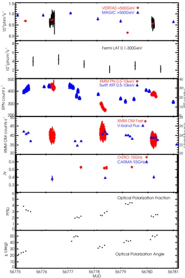
Figure 5. MWL light curves between April 28 and May 4. See the text for details of the light curve in each panel.
calculated as F S F var 2 err 2 2 s = - á ñ á ñ and F N F F N F F 2 4 , F var2 err 2 2 4 err 2 var2 2 var var s = + ás ñ s á ñ + á ñ á ñ
-where S is the standard deviation of the Nflux measurements, err
2
s
á ñ is the mean squared error of theseflux measurements, and
F
á ñ is the meanflux.
The fractional variability results from the simultaneous XMM-Newton and VERITAS data, as well as from con-temporaneous MWL data, are shown in Figure 4. The VHE fractional variability has been computed using the flux light curves integrated above 315 GeV for data from thefirst 3.5 hr on April 29, and above 225 GeV on May 3. The VERITAS fractional variability is ∼13%±3% on April 29, and ∼8%±5% on May 3.
The fractional variability of the X-ray flux is low, but significantly above zero in all three energy intervals 0.5–1 keV, 1–3 keV, and 3–10 keV. Comparing these three X-ray energy intervals, a higher fractional variability is observed at higher frequencies on April 29 (navy open diamonds) and on May 3 (cyan open diamonds), in agreement with previous results (e.g.,
Błażejowski et al. 2005). This may be explained as the manifestation of a different synchrotron-cooling time at different energies, tcool∝E−1/2. In the slow-cooling regime (the cooling time tcoolis longer than the dynamic timescale R/ c), the cooling time is shorter for higher-energy particles, leading to a faster variability in radiation at higher energies. Therefore, more variation at higher energies is observed compared to lower energies on the same timescales, which directly leads to a higher fractional variability for higher-energy emissions. However, the same trend is less obvious on May 1 (blue open diamonds), when only X-ray data are available.
Contemporaneous MWL observations often provide valu-able information about the activity of the source, e.g., abrupt changes in the radio and optical polarizations would reveal the emergence of a compact region that may be connected to a flaring event (see e.g., Arlen et al.2013). MWL light curves of Mrk421 from MJD 56775 to 56781are shown in Figure5. The TeV light curve, measured by MAGIC above 560 GeV on each night before the XMM-Newton observations, is shown in blue in the top panel. The fractional variabilities of the VHEflux for a one-week duration with a 30 minute bin width are measured by both VERITAS and MAGIC are shown as the gray open square and the gray cross in Figure 4, respectively. Only statistical uncertainties are taken into account in the calculation of the VHE fractional variability. As mentioned in Section2.1, the night-to-night systematic uncertainty in the VHE flux measurements from MAGIC in estimated to be ∼11%, the primary contribution to which is the fluctuation of the atmospheric transmission (see Aleksić et al. 2016 for further details). We follow a similar approach and estimate the systematic uncertainty in the VHEflux measured by VERITAS with 10 minute intervals to be less than ∼10% using observations of the Crab Nebula under similar conditions as the observations of Mrk421 in this work. Adding a 10% systematic uncertainty in quadrature to the statistical uncer-tainty of the VERITAS-measured VHE flux reduces its one-week Fvar value from 24.2%±2.5% to 21.9%±3.6%, and the Fvarvalue on April 29 from ∼13%±3% to ∼8%±5%, and the Fvarvalue∼8%±5% on May 3 should be considered as an upper limit.
The daily Fermi-LAT light curve (shown in the second panel) does not suggest any significant variability, although there might be a slight drop in GeV flux after May 1. X-ray count rates from the Swift-XRT are also shown, together with those measured by XMM-EPN in the third panel. The Swift-XRT results fill the gaps between the three XMM-Newton observations, and also show significant variability, illustrated by the fractional variability of∼20% computed from XRT data between April28 and May4, shown as the gray diamond in Figure4. Note that fractional variabilities of∼20% to ∼40% in the X-ray and∼30% in VHE during typical non-flaring states were found by Aleksić et al. (2015a), and much higher values, of∼40% to >60% in both X-ray and VHE during flaring states were found by Błażejowski et al. (2005) and J. Aleksić et al. (2016, in preparation). It is worth noting that fractional variability depends on the bin width, the sampling frequency, and the duration of the light curve(see the discussion section), which makes it more difficult to compare the Fvar values measured using different light curves.
The optical photometric variability of Mrk421 from April 25 to May 4 is mild(see the fourth panel of Figure5). Mrk421 varied from 12.8 to 12.9 in V band, with the maximum optical Figure 6. TeV photon flux vs. X-ray energy flux from the simultaneous
observations on 2014 April 29(shown in navy) and May 3 (shown in cyan). The VHEfluxes are measured by VERITAS integrated above 560 GeV (top panel) and 315 GeV (bottom panel); X-ray energy flux values are converted from the XMM-EPN count rates using ECFs based on the best-fit photon index and neutral hydrogen density of each night. Both X-ray and TeV data are binned in 10 minute intervals.
flux observed on MJD 56775. Over a 24 hr period, the object showed a maximumΔV∼0.1 mag and intra-night variability was generally <0.05 mag. During this period, Mrk421 was close to the middle of the range of optical brightness it has shown since 2008 (V∼11.9–13.6). The source does not exhibit strong variability in the UV band, nor at 15GHz or 95 GHz(see the fourth and fifth panels of Figure5).
In contrast to the flux variations, the optical polarization of Mrk 421 showed more pronounced variability during the dates shown. The observed polarization fraction P peaked at MJD 56779(4%–5%) with minima of P ∼ 2% two days preceding and one day after the polarization maximum(see the sixth panel of Figure 5). The polarization peak reaches only about half of the highest polarization levels observed for this object (10%–13%) since 2008. From 2008 to 2015, the Steward Observatory blazar data archive identified several periods when the polarization of Mrk421 is <1%. Like many blazars, the full range of values for the polarization position angle is exhibited by Mrk421 over a timescale of several years. During the dates shown, the polarization angle χ varied between 20° and 55° with rotations of nearly 20° observed in a day (see the bottom panel of Figure 5). Intra-night variations as large as ∼10° were observed on timescales as short as two hours. During the epoch of the campaign,χ is roughly orthogonal to the position angle of the 43 GHz VLBI jet (∼−35°),68 implying that the magnetic field within the region emitting the polarized optical continuum is more-or-less aligned with the jet.
3.2. Cross-band Flux Correlation
We plot the VHEflux against X-ray count rate in Figure6. There is no significant evidence for correlation. The Pearson correlation coefficient between X-ray flux and TeV gamma-ray flux >560 GeV is 0.48 (the 90% confidence interval is 0.24–0.67), and that between X-ray flux and TeV gamma-ray flux >315 GeV is 0.60 (the 90% confidence interval is 0.35–0.76). The values of the correlation coefficients only suggest a moderate positive correlation, without considering the uncertainties on the measurements. Therefore, we focus on theflux correlations between three X-ray bands, and between two TeV gamma-ray bands, respectively.
3.2.1. Hard/Soft X-Ray Correlation
We further divide XMM-EPN X-ray light curves into three energy bands, 0.5–1 keV, 1–3 keV, and 3–10 keV (as shown in the left panels in Figures 7–9). Z-transformed discrete correlation functions (ZDCFs) between these soft- and hard-X-ray light curves are calculated using a publicly available code, ZDCF v2.2 developed by Alexander (2013), as shown in the right panels in Figures7,8, and 9. At least 11 pairs of light curve points in each time delay bin are required to calculate the ZDCF, zero lag is not omitted, and 1000 Monte Carlo runs were used to estimate the measurement error, in addition to the error calculated in the z-space. From the ZDCFs, the corresponding time lags are calculated using PLIKE v4.0 also developed by Alexander(2013). No significant evidence is Figure 7. Left panel: light curves of Mrk421 observed with XMM-Newton-EPN on 2014 April29. Count rates binned in 50s time intervals in three energy bands, 0.5–1 keV, 1–3 keV, and 3–10 keV, are shown from top to bottom panel, respectively. Right panel: the ZDCF between these three X-ray bands. Positive lag values indicate“hard lag.”
68
found for any leads or lags between the soft-X-ray band relative to the hard-X-ray band.
3.2.2. Gamma-ray Intraband Correlation
The cross-correlations between light curves of blazars at TeV energies are particularly interesting, not only because they can provide insight to the particle acceleration and radiation, but also due to their potential to test Lorentz-invariance violation, which is a manifestation of an energy-dependent speed of light at the Planck scale predicted by foamy structures of spacetime in certain quantum theories (e.g., Aharonian et al. 2008; MAGIC Collaboration et al. 2008; Zitzer for the VERITAS Collaboration 2013).
In a similar fashion as done for the X-ray data(as described in Section 3.2.1), we divide the gamma-ray light curves into two bands, and compute ZDCFs and time lags as shown in Figure10. The chosen bands are 315–560 GeV and 560 GeV– 30 TeV on April 29, and 225–560 GeV and 560 GeV–30 TeV on May 3, so that the event rates are comparable in the higher-and lower-energy bins. ZDCFs are calculated using light curves binned by 10 minutes and 4 minutes, respectively. The 1-σ confidence interval of the time lag of maximum likelihood is calculated between −2000s and 2000s using plike_v4.0. To understand the ZDCFs produced by random noise, we simulate flicker-noise (whose power spectral density (PSD) distribution is proportional to 1/f ) and Gaussian white noise with 10 minute bin width and similar duration as the data. The 95% confidence regions calculated from ZDCF values between 200 pairs of simulated light curves are plotted in Figure 10,
along with ZDCFs calculated from 10 minute binned VER-ITAS light curves above and below 560 GeV. No evidence for time leads or lags is present in the gamma-ray data; however, given the lack of a strong detection of variability, this lack of evidence for any leads/lags is not surprising since the sensitivity to such leads and lags is dependent on the amplitude of the detected variability in these data.
3.3. Hardness Flux Correlation and Spectral Hysteresis Besides the possibility of time lags at different energies, the spectral evolution during blazar flares is also informative. A general trend, that the spectrum is harder when the flux is higher, has been observed in blazars in both the X-ray and gamma-ray bands(e.g., Fossati et al.2008; Acciari et al.2011). Several possibilities can lead to such a trend if the spectrum is being measured at the HE end of the synchrotron and inverse-Compton SED peaks. For example, this could result from an increase in the maximum electron energy, or a hardening in the electron energy distribution. If, however, the X-ray and gamma-ray observations are sampling the emission near the two peaks of the SED, this“harder-when-brighter” effect could also be the result of an increase of the SED peak frequency, which could arise from an increase in magneticfield strength or Doppler factor.
As well as the“harder-when-brighter” trend in the hardness-flux relation, competition between the acceleration and cooling timescales can lead to spectral hysteresis, since the spectral hardness differs on the rising and falling edges offlares (e.g., Kirk et al.1998; Li & Kusunose2000; Sato et al.2008). If one Figure 8. Left panel: light curves of Mrk421 observed with XMM-Newton-EPN on 2014 May1. Count rates binned in 50s time intervals in three energy bands, 0.5–1 keV, 1–3 keV, and 3–10 keV, are shown from top to bottom panel, respectively. Right panel: the ZDCF between these three X-ray bands. Positive lag values indicate“hard lag.”
plots the hardness–flux relation so that the spectrum is harder in the positive y-axis direction, and the flux is higher in the positive x-axis direction, the spectral hysteresis can be seen as a “loop” pattern. Since the spectral hysteresis is driven by the same timescales that determine the time lags at different energies, the direction of the hysteresis loop should be consistent with the sign of the time lag. Specifically, a “hard lag” should correspond to counter-clockwise hysteresis loops (see Section 3.2.1), while a “soft lag” will lead to clockwise hysteresis loops. Therefore, the hardness–flux plot offers an alternative view of the timescales in the system, and can be compared with the time-lag studies presented in the previous section.
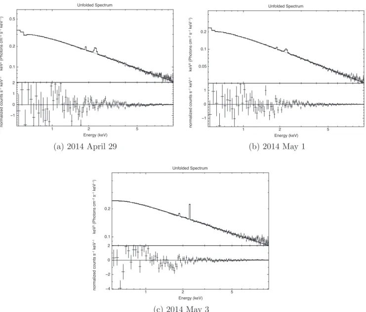
The nightly XMM-Newton-EPN X-ray spectra are fitted using a power-law model with absorption from neutral hydrogen, as well as instrumental features from oxygen, silicon, and gold, following the description in Section 2.3. The results are shown in Figure11and Table4. Note that the equivalent width EWi of each Gaussian component is shown instead of the standard deviation σi, because σi is small compared to the energy-bin size of the X-ray spectrum and therefore not well-constrained by the fit.
We then divide each of the XMM-Newton and VERITAS observations of Mrk421 on the two nights with good atmospheric conditions into simultaneous 10 minute intervals, and perform spectral fitting for each interval, using an absorbed-law model for the X-ray data, and a power-law model for the gamma-ray data. We note that although the X-ray spectral fit is significantly improved by introducing the
extra instrumental features, the spectral indices α remain unchanged within the uncertainty. Therefore we are confident that the hardness ratios and the spectral indices derived for each 10 minute interval are robust, and are not severely affected by the instrumental features.
We identify several time intervals with a rise and a subsequent fall of flux in the X-ray light curves, and plot photon index and hardness ratio againstflux (or count rate) for these bumps(see Figures12and13). Black arrows indicate the order of time for each point. Measurements taken at different times are also color coded to guide the eye. A “harder-when-brighter” effect can be identified on some individual X-ray branches,(e.g., the blue and green points in the top right panel in Figure 12). The observed “soft lag” on May3 indicates a harder spectrum when flux rises, and a softer spectrum when flux falls, corresponding to a clockwise loop (in orange) in the top right panel of the spectral hysteresis plot in Figure 13. Similarly, for the “hard lag” scenario on April29, a counter-clockwise loop is predicted and observed, as shown in Figure12. It is interesting to note that the time lag and loop direction changes forflares separated by a few days, in spite of similarflux levels.
The same analysis has been carried out for VHE data, and similar plots are shown. The uncertainties in VHE flux, hardness ratio, index, and hence hysteresis direction, are large, and do not allow us to draw anyfirm conclusions. We note that although the VHE spectrum of Mrk421 is likely curved, a power-law model describes the data reasonably well for each 10 minute interval(the average reduced χ2value is∼1.05). Figure 9. Left panel: light curves of Mrk421 observed with XMM-Newton-EPN on 2014 May3. Count rates binned in 50 s time intervals in three energy bands, 0.5–1 keV, 1–3 keV, and 3–10 keV, are shown from top to bottom panel, respectively. Right panel: the ZDCF between these three X-ray bands. Positive lag values indicate“hard lag.”
The hardness ratio pattern offers a more crude but less model-dependent estimation of the same signature. However, the hardness–flux diagram of the VERITAS observations also has large uncertainties. At theflux level of roughly 1–2 C. U., such spectral hysteresis studies with the current generation of ground-based gamma-ray instruments is difficult. This offers a reference for the future in defining flux level trigger criteria for ToO observations, aiming for similar goals.
3.4. Power Spectral Density
The PSD can be estimated from a periodogram, which is defined as the squared modulus of the Fourier transform of a time series P F f t t f t t cos 2 sin 2 . N i N i i i N i i 2 1 2 1 2
å
å
n n pn pn = = + = = ⎡ ⎣ ⎢ ⎤ ⎦ ⎥ ⎡ ⎣ ⎢ ⎤ ⎦ ⎥ ( ) ∣ ( )∣ ( ) ( ) ( ) ( )We apply Leahy normalization to the periodogram to get the PSD, so that Poisson noise produces a constant power at an amplitude of 2.
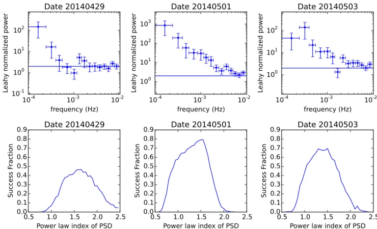
The top panels of Figure14show PSDs calculated from the X-ray light curves of Mrk 421, measured by
XMM-Newton-EPN on 2014 April 29, May 1, and May 3, respectively. The light curves arefirst binned by 50 s intervals, then divided into two equal-length segments, each of 128 bins. A raw power spectrum is calculated for each segment, and averaged over both segments. Then the power spectrum is rebinned geometrically with a step factor of 1.2 (i.e., a bin edge in frequency is the previous bin edge multiplied by a factor of 1.2). To estimate the error of the PSD in each bin, the standard deviation from all PSD points in the bin is used when it contains more than five points, otherwise the theoretical standard deviation of an exponential distribution is used. The PSDs cover a frequency range of 4×10⁻⁴ to 10−2Hz. At higher frequency, the shape of the PSDs becomesflatter due to Poisson noise, which is shown as theflat line with a power of two under the Leahy normalization. However, we note that the PSD is well above the Poisson noise level up to∼10−3Hz on all three days, which corresponds to timescales of under an hour. On May 1, the variability is still present, reaching ∼2–3×10⁻³Hz, which is shorter than 10 minutes.
We then simulate 1000 light curves at each of the indices ranging from 0.5 to 2.5 in steps of 0.1 following Timmer & Koenig (1995), and compare the data and the simulations to compute success fractions (SuFs) as an estimation of the power-law index α following the method described by Uttley et al. (2002). The results are plotted in the bottom panels of Figure14. The SuF peaks at the PSD indices of∼1.5–1.8 on April 29 with a peak value of∼0.5, ∼1.3–1.6 on May1 with a peak value of∼0.8, and ∼1.2–1.6 on May3 with a peak value of∼0.7. These values represent the indices of the PSD better than the simple power-law fit to the PSD, as SuFs are less biased by the spectral leakage which is present in both the data and the simulations. The range of PSD indices is consistent with previous studies of the same source at lower frequencies, e.g., a PSD index of 1.35–1.85 was found for frequency range ∼10−8–2×10⁻⁶Hz(Isobe et al. 2015). However, a break at frequency of∼9.5×10⁻⁶Hz was found in the X-ray PSD of Mrk 421 by Kataoka et al.(2001), and the PSD index above this frequency was determined to be 2.14. Surprisingly, we do notfind evidence of such a steep PSD at 4×10⁻⁴Hz.
3.5. Broadband SEDs
The SED of simultaneous VERITAS and XMM-Newton data, as well as contemporaneous MWL data, is shown in Figure15. Daily averaged HE (∼30 MeV–100 GeV) gamma-ray spectra are constructed from Fermi-LAT data between 100 MeV and 300 GeV, and butterfly regions of 95% confidence level are shown. Note that the uncertainty is large because of the scarcity of HE photons in the one-day window. Optical spectra from the Steward Observatory between 400 and 750 nm on May3, radio data from CARMA at 95GHz taken on both nights, and from OVRO at 15GHz on other nights within the week are also shown.
The X-ray and VHE spectra are located at the falling slopes of the lower- and higher-energy spectral peaks, respectively. The synchrotron peak is between the UV measurement at ∼1015Hz and the soft end of the X-ray spectrum at∼1017Hz. Although the Fermi-LAT spectrum is not very constraining, the HE spectral peak appears to be just below ∼100 GeV, as suggested by the TeV spectrum.
We use a static SSC model described in Krawczynski et al. (2002) to study the observed SEDs. The set of parameters used to generate the solid blue and red curves as shown in Figure15 Figure 10. VERITAS ZDCFs between light curves integrated below and above
560 GeV of Mrk 421 on 2014 April29 and May3. The 95% confidence region fromflicker noise and white noise simulations are shown as red dashed lines and green dotted lines, respectively.
Figure 11. X-ray spectra of Mrk 421 measured by XMM-Newton-EPN from the three simultaneous ToO observations in 2014. The spectra are fitted with a power-law plus absorption model accounting for the source, and multiple instrumental features(see the text and Table4for details).
Table 4
XMM-Newton-EPN Spectral Fit Results and ECFs using the Absorbed-power-law Model Plus Three Instrumental Features Described in Equation(2)
Parameter Unit Value on 56776 Value on 56778 Value on 56780
Ec keV 0.540±0.003 0.530±0.003 K D L 0.118±0.005 0.146±0.009 K E0,0 keV K K 0.48±0.04 EW0 keV K K <0.11 KG,0 10−3 K K 0.022±0.015 nH 10 20 cm−2 1.9 1.9 1.9 α L 2.649±0.002 2.817±0.004 2.450±0.002 KPL L 0.2714±0.0004 0.1711±0.0004 0.2251±0.0002 E0,1 keV 1.88±0.02 1.88±0.02 1.87±0.03 EW1 eV 4±2 4±3 2±2 KG,1 10−4 2.2±0.4 1.1±0.4 0.9±0.5 E0,2 keV 2.26±0.01 2.25±0.01 2.26±0.01 EW2 eV 26±3 19±3 19±7 KG,2 10−4 8.1±0.4 3.3±0.4 5.9±0.6 Reducedχ2 L 1.6 1.3 2.3
Note. Note that the fits are insensitive to the width σiof the Gaussian component, therefore the equivalent width(EW) values are shown instead. The instrumental feature around 0.5 keV isfitted as an edge component on MJD 56776 and 56778, but as a Gaussian component on 56780.
are listed in Table5. The static one-zone SSC model is roughly consistent with the data. The synchrotron peak frequency given by the model is νsyn∼4×10¹⁶Hz, while the inverse-Compton peak lies at νSSC∼5×1025Hz. Using the peak frequencies and the observed spectral indices below and above the synchrotron peak, we can follow Equation (16) given by Tavecchio et al. (1998) assuming the system is in the Klein– Nishina(KN) regime and estimate the strength of the magnetic field to be B mc h z 2.7 10 exp 1 1 1 2 1 1 0.06 G, 7 syn SSC 2 2 2 1 2 1 2 dn n a a a » ´ ´ - + - + » - ⎛ ⎝ ⎜ ⎞ ⎠ ⎟ ⎧ ⎨ ⎩ ⎡ ⎣⎢ ⎤ ⎦⎥ ⎫ ⎬ ⎭ ( )
where d= G[ (1-b cosq)]-1 »20.3 is the Doppler factor (Γ and θ taken from the SED modeling results on May 3), α1∼0.5 and α2∼1.5 are the observed spectral indices below and above the synchrotron peak. We also calculate the Doppler factor limits for the KN and Thomson regimes to be∼13 and ∼29, respectively, following Equations (13) and (17) in Tavecchio et al. (1998). The Doppler factor value of 20.3 obtained from the SSC model is in between the two limits,
therefore the gamma-ray emission is in the Thomson-to-KN transition regime.
From April 29 to May 3, the change in SED might be described by an increase in the radius of the emitting region R, along with an increase in the maximum energy Emax, a slight decrease in break energy Ebreakof the electron distribution, a harder electron spectrum (smaller p2) after the break energy, and a slight increase in the Doppler factor(see Table5). Note that a slight increase in magnetic field strength can have a similar effect as the increase in the Doppler factor. If these parameters indeed describe the evolution of the SED, it is consistent with the results of an expansion of the emitting region. The direct result of such an expansion is an increase in the dynamic timescale tdyn= R/c. Moreover, this will lead to a higher maximum energy of the electrons Emax, since the maximum possible gyro-radius has increased. Also, the synchrotron cooling break, which occurs at the electron energy that satisfies tsyn= tdyn, decreases since tsyn∝γ−1, whereγ is the Lorentz factor of the electron.
Under the simple SSC model, the hypothesis of an increase in the maximum energy Emax would be consistent with a counter-clockwise spectral hysteresis pattern on April 29 and a clockwise pattern on May 3. The former is predicted when the system is observed near the maximum particle energy(see e.g., Kirk et al. 1998), in which case the increasing acceleration timescale with higher particle energy results in the higher-Figure 12. Spectral hysteresis of Mrk 421 on 2014 April 29. The top and bottom rows show results from X-ray and TeV observations, respectively. In each row, the left plot shows a light curve segment that contains a bump influx, the middle plot shows the relationship between flux (counts) and best-fit photon index, and the right plot shows the relationship betweenflux (counts) and the hardness ratio. Each point of flux, HR, and index measurement is from a 10 minute interval. The hardness ratio for X-ray is the ratio between the count rates in 1–10 keV and 0.5–1 keV; and for VHE between 560 GeV–30 TeV and 315–560 GeV. Black arrows and different colors are used to guide the eye as time progresses.
energy photons lagging behind the lower-energy ones. Consequently, this leads to a softer spectrum when flux rises because lower-energy photons are emitted faster, and a counter-clockwise spectral hysteresis pattern. If the maximum electron energy Emax is lower on April 29, the observed X-ray frequency (fixed at 0.5–10 keV) is closer to the maximum frequency, therefore the change influx propagates from low to high frequencies and a counter-clockwise spectral hysteresis pattern should be observed. On the other hand, on May 3, as Emax increases, the observed X-ray frequency covers a relatively lower portion of the entire particle spectrum, therefore the change in flux propagates from high to low energies and a “soft lag” may be observed.
4. DISCUSSION
A detailed blazar variability study on sub-hour timescales using simultaneous and continuous VHE and X-ray observa-tions has been presented in this work. Although it is challenging to carry out studies on such short timescales, they have the potential to constrain blazar models. Several different analyses in time and energy space are carried out, providing results that can cross-check each other. Although the VHEflux level and dynamic range in this work are not sufficient to provide a conclusive picture of the emission mechanisms, the
methods used are important for similar observations if the source is at higherflux levels and/or more variable.
At theflux level of roughly ∼2C.U., Mrk421 shows <20% fractional variability in VHE gamma-ray flux on sub-hour to hour timescales, which seems low compared to previous studies on longer timescales at even lower fluxes. However, this is expected as the PSD of the variability follows a 1/fα style power law, leading to a lower variability power at higher frequencies(i.e., on shorter timescales) given that the value of α ranges from ∼1.2 to ∼1.8. For example, if a PSD of 1/f1.5 holds from∼1.65×10⁻⁶Hz (1 week) to 0.01Hz (50 s), the fractional variability from timescales of 7 days down to 1 day would be∼12 times higher than that from timescales probed in the XMM-Newton observations in this work. However, rare incidences of fast and strong variability in both X-ray and VHE have been observed before, e.g., variability with an amplitude of ∼15% and on timescales of 20 minutes was reported by Błażejowski et al. (2005). Such fast flares could be the manifestation of 1/fαnoise or individual local events caused by a different process. A steepening of the X-ray power spectral index to α∼2.14 at 9.5×10⁻⁶Hz for Mrk421 was reported by Kataoka et al.(2001). Such break features in the PSD of AGNs potentially carry information about the emission mechanism or characteristic timescales of the system. However, we do notfind evidence of a much steeper PSD at Figure 13. Spectral hysteresis of Mrk 421 on 2014 May 3. The top and bottom rows show results from X-ray and TeV observations, respectively. In each row, the left plot shows a light curve segment that contains a bump influx, the middle plot shows the relationship between flux (counts) and best-fit photon index, and the right plot shows the relationship betweenflux (counts) and the hardness ratio. Each point of flux, HR, and index measurement is from a 10 minute interval. The hardness ratio for X-ray is the ratio between the count rates in 1–10 keV and 0.5–1 keV; and for VHE between 560 GeV–30 TeV and 225–560 GeV. Black arrows and different colors are used to guide the eye as time progresses.
4×10⁻⁴Hz, compared with previous studies of the same source at lower frequencies.
Several important timescales in blazars—the cooling time tcool, acceleration time tacc, dynamic timescale tdyn, and
injection timescale tinj—control many of the observable quantities, including the energy-dependent trends in their variability. For example, if the cooling timescale controls the flare timescale (the slow-cooling regime), a shorter decay timescale and greater fractional variability will be observed at higher energies, and a “soft-lag” and clockwise spectral hysteresis loop will be seen(e.g., Kirk et al. 1998). “Soft-lag” has been commonly observed in blazars in the X-ray band (e.g., Falcone et al.2004), although “hard-lag” has also been reported (e.g., Sato et al. 2008). Spectral hysteresis has also been observed from blazars, mostly from HBLs in the X-ray band(e.g., Cui2004), as well as from a few flat-spectrum radio quasars in the HE gamma-ray band (e.g., Nandikotkur et al.2007).
Within this work we attempt to measure spectral hysteresis patterns, as well as leads/lags between higher- and lower-energy bands, within both X-ray and VHE gamma-ray regimes, using the simultaneous ToO observations of Mrk 421 in these two bands in 2014. However, the lack of significant detection of time lags using two cross-correlation methods suggests that, at the observedflux level (roughly between 1 and 2 C. U.) and fractional variability amplitude (15%), the current ground-based gamma-ray instruments are still not sensitive enough for such studies. Future gamma-ray observations with current instruments at higherflux levels or with greater dynamic range, e.g., during aflare similar to the 10 C.U. TeV gamma-ray flare from Mrk 421 that lasted for∼1 hr (Gaidos et al.1996), or with more sensitive instruments, e.g., the Cherenkov Telescope Figure 14. The PSD distributions (top row) and success fraction results (bottom row) of Mrk421 calculated from the XMM-Newton-EPN observations in 2014. The power spectra are averaged over two segments of light curves each with 128 bins, and then rebinned geometrically in frequency space with a step factor 1.2. The PSDs are Leahy normalized, and theflat lines indicate the power of Poisson noise. The success fraction (SuF) results are calculated from comparisons between data and simulated light curves assuming an underlying PSD that follows a power-law distribution, the index of which goes from 0.5 to 2.5 in 0.05 steps. The highest frequencies(>2×10⁻³Hz,>7×10⁻³Hz, and>3×10⁻³Hz on April 29, May 1, and May 3, respectively) are excluded when calculating the SuF to get rid of the bias caused by white noise. A total of 1000 simulated light curves are generated at each index.
Figure 15. Broadband SED of Mrk 421 on 2014 April 29 (shown in blue) and May 3(shown in red). From higher frequencies to lower ones, filled circles show VERITAS data, butterfly regions show Fermi-LAT data averaged over one day, round dots and triangles show XMM-Newton-EPN and OM data, respectively, small dots show Steward Observatory data(only on May 3, with host galaxy subtracted), and squares show CARMA and OVRO data. See text for details of the measurements and the SSC models shown. The results from previous observations are also shown for comparison: the gray, green, and magenta dashed lines correspond to models used for high, medium, and low flux as described in Błażejowski et al. (2005).