Dipartimento di
Scienze Chimiche, Biologiche, Farmaceutiche ed Ambientali
“Doctor of Philosophy in “Chemical Sciences”
Optimization, Evaluation and Use of Advanced Gas
Chromatography-Mass Spectrometry Methods within the
Context of Food Analysis
Ph.D. Thesis of:
Barbara Giocastro
Supervisor:
Prof. Luigi Mondello
Coordinator:
Prof.ssa Paola Dugo
Optimization, Evaluation and Use of Advanced Gas Chromatography-Mass Spectrometry Methods within the Context of Food Analysis
TABLE OF CONTENTS
Chapter 1
General scope and introduction ... 1
References ... 4
Chapter 2 Comprehensive two-dimensional gas chromatography: fundamentals and theoretical/practical aspects ... 5
2.1. Gas chromatography fundamentals ... 5
2.1.1. GC terminology and figures-of-merit ... 6
2.2. The need for multidimensional GC ... 16
2.3. From MDGC to GC×GC ... 17
2.4. GC×GC: basic instrumental setup ... 22
2.4.1. Column combination ... 24 2.4.2. Transfer device ... 28 2.4.3. Detectors ... 28 2.5. Modulators ... 30 2.5.1. Thermal modulators... 32 2.5.1.1. Cryogen-based modulators ... 34 2.5.1.2. Cryogen-free modulators... 39 2.5.2. Valve-based modulators ... 42
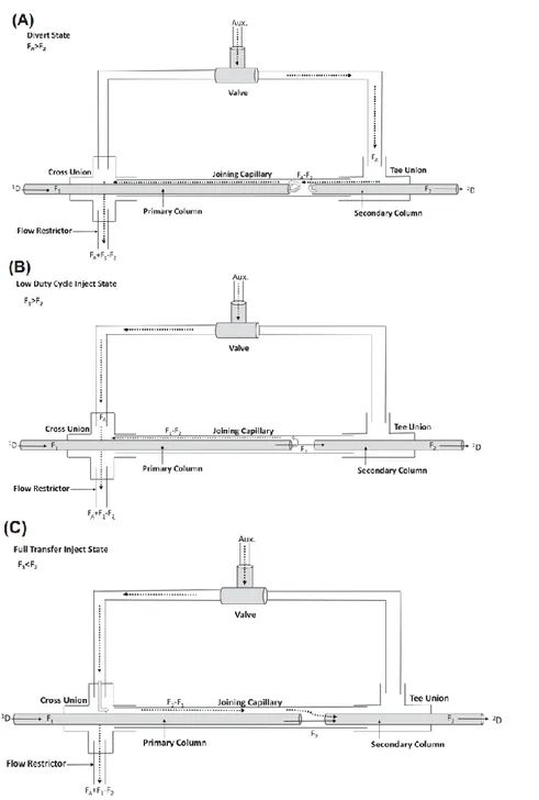
2.5.2.1. Differential flow modulation ... 43
2.5.2.2. Flow diversion modulation... 45
2.5.3. Optimization aspects ... 50
2.5.3.1. Modulation parameters ... 50
2.5.3.2. Modulator type ... 51
References ... 54
Chapter 3 GC×GC-mass spectrometry hyphenation ... 59
3.1. Introduction ... 59
3.2. Mass Spectrometry Fundamentals ... 61
3.2.1. Mass resolution and mass accuracy ... 63
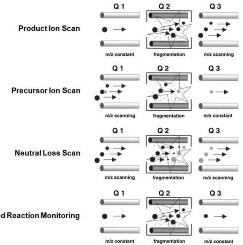
3.3. Ionization modes ... 64 3.3.1. Electron ionization... 65 3.3.2. Chemical ionization ... 67 3.4. Mass Analyzers ... 69 3.4.1. Single quadrupole ... 70 3.4.2. Time-of-flight ... 73 3.4.3. Triple quadrupole ... 76
3.5. Evolution and current state of GC×GC-MS ... 78
Research in the field of advanced chromatography-mass spectrometry technologies
for food samples analysis ... 85
4.1. In-depth qualitative analysis of essential oils using LC// GC×GC-QMS ... 85
4.1.1. Experimental ... 87
4.1.2. Results and Discussion ... 89
4.2. Chemical characterization of lipid profile in unconventional palm-oils using CM-GC×GC-QMS ... 98
4.2.1. Experimental ... 100
4.2.1.1. Fatty acids (FAs) analysis ... 101
4.2.1.2. Carotenoids analysis ... 102
4.2.2. Results and Discussion ... 104
4.2.3. Conclusions ... 110
4.3. GC×GC-HR-TOF MS: exploring the chemical signature of food cooking emissions ... 111
References ... 116
Chapter 5 Towards the determination of an equivalent standard column set between cryogenic and flow modulated GC×GC-MS ... 119
5.1. Analysis of coconut-derived bio-oil by using flow- and cryogenic-modulation comprehensive 2D gas chromatography-mass spectrometry ... 119
5.1.1. Introduction ... 120
5.1.2. Material and methods ... 121
5.1.2.1. Sample, standard compounds, and sample preparation ... 121
5.1.2.2. Instrumentation ... 121
5.1.3. Results and Discussion ... 124
5.1.4. Conclusions ... 132
5.2. Analysis of fragrance allergens by using flow- and cryogenic-modulation comprehensive 2D gas chromatography-mass spectrometry: obtaining similar chromatography performances ... 133
5.2.1. Experimental ... 133
5.2.1.1. Standard compounds and sample preparation ... 133
5.2.1.2. Instrumentation ... 134
5.2.2. Results and Discussion ... 135
5.2.3. Conclusions ... 142
Optimization, Evaluation and Use of Advanced Gas Chromatography-Mass Spectrometry Methods within the Context of Food Analysis
Chapter 6
Research in the field of comprehensive 2D GC-MS using milder electron ionization
conditions ... 145
6.1. Introduction ... 145
6.2. Experimental ... 147
6.2.1. Sample, standard compounds, and sample preparation ... 147
6.2.2. Instrumentation ... 148
6.3. Results and Discussion ... 149
6.3.1. Phytosterols ... 150
6.3.2. Fatty acid methyl esters ... 152
6.3.3. Hydrocarbons, pesticides and other compounds ... 154
6.4. Conclusions ... 159
References ... 160
Chapter 7 Research in the field of fast comprehensive 2D GC-MS: concept, method optimization, and application ... 163
7.1. Introduction ... 163
7.2. Experimental ... 165
7.3. Results and Discussion ... 166
7.4. Conclusions ... 173
References ... 174
Chapter 8 Evaluation of a novel consumable-free thermal modulator: gas flow optimization aspects 175
8.1. Evaluation of different internal diameter uncoated modulation columns within the context of solid state modulator ... 175
8.1.1. Introduction ... 176
8.1.2. Material and methods ... 177
8.1.3. Results and Discussion ... 178
8.1.3.1. 0.20 mm id modulation column ... 179
8.1.3.2. 0.25 mm id modulation column ... 181
8.1.4. Conclusions ... 185
8.2. Evaluation of different internal diameter coated modulation columns within the context of solid state modulator ... 185
8.2.1. Experimental ... 186
8.2.2. Results and Discussion ... 187
8.2.2.1. Outline of the research ... 187
8.2.2.2. Isothermal analysis ... 188
8.2.2.3. Temperature-programmed analysis ... 192
8.2.3. Conclusions ... 196
References ... 197
All figures and tables have been reproduced with the permission of Elsevier,
John Wiley and Sons and ACS publications
Chapter 1
General scope and introduction
The field of food analysis is characterized by heterogeneous samples, ranging from samples of relatively low complexity and other highly challenging ones (e.g. roasted coffee aroma,etc.) which usually contain hundreds of compounds in a wide range of concentrations. In
general, food products consists of many different nutrients of organic (e.g. lipids, carbohydrates, proteins, vitamins etc.) and inorganic (e.g. water, minerals, oxygen) nature. In addition to natural constituents, food products may contain cooking-related compounds (e.g. Maillard reactions products), xenobiotic substances that come mainly from technological processes, agrochemical treatments or packaging materials (e.g. phytosanitary products, plastic derivatives, mineral oil, etc.) and undesired transformation products (e.g., oxidization, isomerization, and hydrolysis). All of these substances present abroad molar mass range, variable polarity, and a wide range of chemical abundance. The identification of such compounds in complex food samples, remains challenging in the field of food analysis. At present, one-dimensional (1D) gas chromatography (GC) is widely exploited for the separation of volatile and semi-volatile species in food products. However, often the complexity of many naturally occurring matrices exceeds the capacity of any single separation system. Therefore, in the past years considerable research has been directed to the combination of independent techniques, with the aim of strengthening resolving power. In such a respect, to circumvent the sample complexity an advisable option is the use of multidimensional analytical techniques. In such a respect, comprehensive two-dimensional gas chromatography coupled to various forms of mass spectrometry (GC×GC-MS) is one of the most powerful analytical tools available for the separation of complex food samples.Comprehensive 2D GC was first described in 1991 [1], when Liu and Phillips employed dual-stage thermal modulation to achieve a GC×GC separation. Since its inception, many efforts have been made in the field of GC×GC in terms of hardware, software and practical/theoretical studies.
The aim of the general research, described in this Ph.D. thesis, is the optimization, evaluation and use of advanced gas chromatography-mass spectrometry methods within the context of food analysis. Moreover, focus was dedicated to various optimization aspects of GC×GC-MS. Specifically, I have been involved in a study focused on the off-line combination of normal phase high performance liquid chromatography (NP-HPLC) and GC×GC coupled with quadruple mass spectrometry detection (QMS) [2], for the detailed qualitative profiling of the entire volatile fraction of essential oils. Apart from essential oils, cryogenic-modulated (CM) GC×GC-QMS has been exploited for the chemical characterization of lipid fatty acids in unconventional palm oils [3].
A further study was related to the optimization aspects within the context of different modulator devices. Modulators are the “key” component of any GC×GC system, with cryogenic and flow modulation (FM) the two most employed devices. In such a respect, the goal of the work was to generate similar chromatography profiles using finely-tuned CM- and FM-GC×GC-MS experimental conditions, with emphasis directed to the challenge of defining an equivalent column set. In this context, a side-by-side measurement of several chromatography parameters was carried out on a sample of coconut-derived bio-oil (a food-waste sample) [4] and on a mixture of cosmetic allergens [5].
I was involved in a review article focused on the current trends in the field of GC×GC-MS [6]. Attention was devoted to various aspects of mass spectrometry, in particular to ionization processes. Later, my activity moved towards the use of “milder” electron ionization conditions in the GC×GC-QMS analysis of a variety of different molecular-mass compounds with various polarities contained in vegetable oil (e.g., sterols, fatty acid methyl esters, vitamin E, squalene, and a linear alcohol) [7]. The use of “milder” ionization enhances the possibility to add a further level (or point) of identification in GC×GC-QMS, namely the molecular mass, thus facilitating the detailed profiling of several complex food samples.
In addition, I was involved in a study in the field of fast GC×GC-QMS, developing a method based on the use of micro-bore columns in both dimension for the analysis of fragrance allergens [8]. Finally, I dedicated my activity on a research focused on the evaluation of a novel form of consumable-free thermal modulation, namely solid-state modulation (SSM) [9]. Specifically, the effect of gas flow conditions on SSM performance was evaluated in relationship to different modulation column geometries.
I was involved in a research focused on the analysis of pollutants released from food cooking emissions. The research work was carried out within the context of an internship at Helmholtz Zentrum Muenchen under the supervision of Prof. Ralf Zimmermann. It must be noted that, due to the corona virus pandemic, the research work was interrupted and only a brief description of the initial research project is herein reported.
References
[1] Z. Liu, J.B. Phillips. J. Chromatogr. Sci. 29 (1991) 227.
[2] M. Zoccali, B. Giocastro, I. L. Bonaccorsi, A. Trozzi, P. Q. Tranchida, L. Mondello, Foods, 8 (11) (2019) 580.
[3] Y. Caro, T. Petit, I. Grondin, P. Clerc, H. Thomas, D. Giuffrida, B. Giocastro, P. Q. Tranchida, I. Aloisi, D. Murador, L. Mondello &L. Dufossé. Nat. Prod. Res. 34 (2020) 93. [4] I. Aloisi, T. Schena, B. Giocastro, M. Zoccali, P. Q. Tranchida, E. B. Caramāo, L. Mondello, Anal. Chim. Acta 1105 (2020) 231.
[5] B. Giocastro, I. Aloisi, M. Zoccali, P. Q. Tranchida, L. Mondello, LC-GC (Europe) 33 (10) (2020) 512.
[6] P. Q. Tranchida, I. Aloisi, B. Giocastro, L. Mondello, TrAC Trends Anal. Chem. 105 (2018) 360.
[7] P. Q. Tranchida, I. Aloisi, B. Giocastro, M. Zoccali, L. Mondello, J. Chromatogr. A 1589 (2019) 134.
[8] B. Giocastro, M. Piparo, P. Q. Tranchida, L. Mondello, J. Sep. Sci. 41 (2018) 1112. [9] M. Zoccali, B. Giocastro, P. Q. Tranchida, L. Mondello, J. Sep. Sci. 42 (3) (2019) 691.
Chapter 2
Comprehensive two-dimensional gas
chromatography: fundamentals and
theoretical/practical aspects
2.1 Gas chromatography fundamentals
Gas chromatography (GC), with open-tubular capillaries (OTC), is the technique of choice for the separation of volatile and semi-volatile compounds that are thermally stable at the temperatures required for their vaporization. The milestone work focused on GC was first published in 1952 [1] when Martin and James acted on a suggestion made 11 years earlier by Martin himself in a Nobel-prize winning paper on partition chromatography [2]. In the early days, GC remained exclusively a packed-column technique and not substantially different from the initial work of Martin and James. In 1958, Golay introduced the use of the open-tubular columns, demonstrating that a tube of capillary dimensions coated with a thin film of liquid was capable of providing superior efficiency to a packed column [3]. The schematic representation of a gas chromatograph setup is shown below in
Figure 2.1. At the heart of the system is the column, in which the crucial physicochemical
process of the separation occurs. The column contains the stationary phase, while the mobile phase (the carrier gas) is flowing through this column from a pressurized gas cylinder (source of the mobile phase). A pressure and/or flow-regulating unit controls the rate of mobile-phase delivery. The introduction of the sample is performed through a unit called injector. The whole sample is transferred from the injector to the analytical column, where continuous redistributions between the mobile phase and the stationary phase occur. Due to their different affinities for the stationary phase the individual components, eventually, form their own concentration bands, which reach the column’s end at different times. The analytical column is directly connected to the detector, which identify and/or quantify the single components eluting from the separating column.
Figure 2.1. The main components of a gas chromatograph.
Summarizing the above, a typical gas chromatograph, essentially consist of three independently controlled thermal zones:
i) the injector zone that ensures rapid volatilization of the introduced sample;
ii) the column temperature that is controlled to optimize the separation process and
iii) the detector zone that must be at temperatures where the individual sample components are measured in the vapour phase.
2.1.1 GC terminology and figures-of-merit
- Retention
Separations by gas chromatography are recorded as chromatograms, of which an example is provided in Figure 2.2. Such a chromatogram is, basically, a plot of a series of peaks representing the separated compounds ordered by increasing time for elution (retention time) along the x-axis, vs. the detector response to the compounds as the y-axis.
Figure 2.2. GC chromatogram example.
The observed retention time (tr) contains the contribution of three components, which are related to the column and system properties:
i) the extra column retention time (the time to transport the sample to and from the column to accomplish sample introduction and detection);
ii) the column holdup time, the so-called dead time (the time required to transport a compound with no interactions with the stationary phase the length of the column), and
iii) the adjusted retention time (the additional time other than for transport each compound is delayed on account of its interactions with the stationary phase).
To characterize retention properties, regardless of the system characteristics, a useful term is the retention factor, k’, defined as:
𝑘′ =𝑡𝑟− 𝑡0 𝑡0
(Eq. 2.1)
the ratio of the time a compound engages in interactions with the stationary phase during the duration of separation, [or adjusted retention time (𝑡𝑟− 𝑡0)], and the time it takes a
completely unretained analyte in the carrier gas stream to travel the length of the column (dead time). Analytes with small k’ will have little affinity for the stationary phase and shorter 𝑡𝑟. Analytes with large k’ spend more time retained by the stationary phase and have longer 𝑡𝑟.
A measure of column selectivity is provided by the separation factor, α. The α value is obtained by a simple calculation corresponding to the ratio of the retention factors 𝑘′, for any two compounds, with the numerator always the more retained of the two compounds. The term α can have values ≥1; a value of 1 corresponds to co-elution, indicating that the column has no selectivity for the separation.
The distribution constant Kc is a thermodynamic parameter defined as:
𝐾𝑐 = 𝐶𝑠⁄𝐶𝑀
(Eq. 2.2)
where the terms Cs and CM are equal to the solute concentration in the stationary and mobile
phases, respectively.
The distribution constant, Kc, is connected to the retention factor, k’, by the following
expression:
𝐾𝑐 = 𝑘’ × 𝛽
(Eq. 2.3)
where 𝛽 is the phase ratio which is given approximately by dividing the column radius by twice the film thickness for open-tubular columns:
𝛽 = 𝑟𝑐⁄2𝑑𝑓
(Eq. 2.4)
Since the early days of gas chromatography, an enormous effort has been directed at standardizing retention measurements to facilitate the use of collections of retention data for compounds identification. The retention index is the best method for documenting the GC properties of any compound. In the case of isothermal analysis, the retention index can be calculated as reported in Eq. 2.5. The retention index compares retention of a given solute (on a logarithmic scale) with the retention characteristics of standard solutes solution that usually are a homologous series of compounds:
𝐼 = 100𝑧+ 100
log 𝑡𝑟(𝑥)− log 𝑡𝑟(𝑧) log 𝑡𝑟(𝑧+1)− log 𝑡𝑟(𝑧)
(Eq. 2.5)
The term z corresponds to the number of carbon atoms within a homologous series, while
x relates to the unknown. For example, a series of n-alkanes can be used in this direction;
each member of a homologous series (differing in a single methylene group) being assigned an index value of 100 times its carbon number (e.g., 100 for methane, 200 for ethane, and 300 for propane, etc.). If a given solute happens to elute from the column exactly half-way between pentane and hexane, its retention index value is 550.
- Band broadening
The success of any GC separation is primarily dependent on maximizing the differences in retention times of the individual mixture components. Analytes are detected following the GC separation exhibiting an approximately Gaussian concentration distribution, defined by their tr and the width at the base of the corresponding chromatographic peak, Wb.
The analyst aims to minimize peak broadening, measured as Wb in order to maximize the
number of analyte peaks that can be ideally placed, side-by-side, into the available separation space, at a given resolution (peak capacity, nc). Whereas the retention times are
mostly related to the thermodynamic properties of the separation column, the peak width is a function of the efficiency of the solute mass transport from one phase to the other one and of the kinetics of sorption and desorption processes. In the case of OTC, the width of a chromatographic peak is determined by various processes such as molecular diffusion in the gas phase, molecular diffusion in the stationary phase, the residence time in the stationary phase, and the parabolic flow profile of the carrier gas along the column. The most widely used, criterion of the column efficiency is the number of theoretical plates,
N. Figure 2.3 shows the measurements needed to calculate the value of N from a
chromatographic peak. N = (tr 𝜎) 2 = (tr 𝑊𝑏) 2 16 = 5.54 (tr 𝑊ℎ) 2 (Eq. 2.6)
Different terms arise because the measurement of σ can be made at different heights on the peak; at the base of the peak, 𝑊𝑏 is 4σ, so the numerical constant is 16 (42); at half height, 𝑊ℎ is 2.35 σ, so the constant becomes 5.54 (please refer to Figure 2.3).
Figure 2.3. Determination of the number of theoretical plates of a chromatographic column.
A related parameter which express the efficiency of column is the plate height, H,
𝐻 = 𝐿/𝑁
(Eq. 2.7) where L is the column length. The length of a chromatographic column L is viewed as divided into imaginary volume units (plates) in which a complete equilibrium of the solute between the two phases is attained. Obviously, for a given value of tr, narrower peaks
provide greater numbers of theoretical plates than broader peaks.
For the sake of simplification, in the previous equations, the peak is assumed as perfectly symmetrical, following a Gaussian distribution, but real peaks usually exhibit some asymmetry (Figure 2.4), which are easily handled by peak modelling approaches [4].
Figure 2.4. Departures from peak symmetry: (a) slow desorption process (tailing) and (b) column overloading (fronting). (c) Gaussian distribution.
The earliest attempts to examine the efficiency of column explain chromatographic band broadening were based on a kinetic approach described by the van Deemter Equation:
𝐻 = 𝐴 +𝐵
ū+ 𝐶ū
(Eq. 2.8)
The broadening was expressed in terms of the plate height, H, as a function of the average linear gas velocity ū. The van Deemter Equation was referred to packed columns only and it identified three effects that contribute to the band broadening. The eddy diffusion (term
A) describes the chromatographic band dispersion caused by the gas-flow irregularities in
the column; the longitudinal molecular diffusion (term B) represents the peak dispersion due to the diffusion processes occurring longitudinally inside the column, and the mass
transfer in the stationary liquid phase (C-term) which occurs due to a radial diffusion of
the solute molecules. Thus, each of the three terms (A, B and C) should be minimized in order to maximize the number of theoretical plates, thus column efficiency.
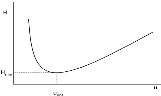
A hyperbolic plot, the so-called van Deemter curve (Figure 2.5), represents the influence of linear gas velocity (ū) on the band broadening (Eq. 2.8). The curve shows the existence of an optimum velocity (ū) at which a given column exhibits its highest number of theoretical plates (N). Shapes of the van Deemter curves are further dependent on a number of variables: solute diffusion rates in both phases, column dimensions and various geometrical constants, the phase ratio, and retention times.
Figure 2.5. Relationship of the plate height and linear gas velocity (van Deemter curve).
Open-tubular columns contain no packing material inside the column and the A-term becomes zero, reducing the van Deemter equation to a form known as Golay Equation [5]. Specifically, two C-terms were introduced in the equation; one for the mass transfer in the stationary phase, Cs (similar to van Deemter), and one for mass transfer in the mobile phase, Cm. Thus the Golay Equation is:
𝐻 =𝐵
ū+ (𝐶𝑠+ 𝐶𝑚)ū
(Eq. 2.9)
where B-term represents the molecular diffusion. The equation governing molecular diffusion is:
𝐵 = 2𝐷𝐺
where DG is the diffusion coefficient for the solute in the carrier gas. In Eq. 2.9, this term is
divided by the linear velocity (ū), so a large velocity or flow rate will also minimize the contribution of the B-term to the overall peak broadening. That is, a high velocity (ū) will decrease the time a solute spends in the column and thus decrease the time available for molecular diffusion. The Cs term refers to mass transfer of the solute in the stationary phase
and it is defined as Cs = 2kdf 2 3 + (1 + k)2D s (Eq. 2.11)
where df is the average film thickness of the liquid stationary phase and Ds is the diffusion
coefficient of the solute in the stationary phase. To minimize the contribution of this term, the film thickness should be small and the diffusion coefficient large. Rapid diffusion through thin films allows the solute molecules to stay closer together. Typical values for film thickness fall into the range 0.05–5 μm. Some typical performance properties for different open-tubular columns are reported in Table 2.1. The other part of the CS-term is the ratio k/(1 + k)2. Large values of k result from high solubilities in the stationary phase. This ratio is minimized at large values of k, but very little decrease occurs beyond a k value of about 20. Since large values of retention factor result in long analysis times, little advantage is gained by k-values larger than 20.
Golay‘s equation for the Cm term is:
𝐶𝑚 =(1 + 6𝑘 + 11𝑘 2)𝑟 𝑐2 24(1 + 𝑘)2𝐷 𝐺 (Eq. 2.12)
where rC is the radius of the column. The relative importance of the two C-terms in the rate
equation depends primarily on the film thickness and the column radius. We can say that for thin films (< 0.2 μm), mass transfer controls the C-term in the mobile phase; for thick films (2-5 μm), it is controlled by mass transfer in the stationary phase; and for the intermediate films (0.2 to 2 μm) both factors need to be considered. For the larger wide bore columns, the importance of mass transfer in the mobile phase in considerably greater. Finally, another consideration can be made on the C-terms that are multiplied by the linear velocity in Eq. 2.9: they are minimized at low velocities and so there is much time for the
molecules to diffuse in and out of the liquid phase and to diffuse across the column in the mobile gas phase.
Table 2.1. Typical performance characteristics for 30 m coated OTC measured for n-undecane at 130°C.
Internal diameter (mm)
Film thickness
(µm) Phase ratio Column (N)
0.10 0.10 249 480000 0.10 0.25 99 328500 0.25 0.25 249 192000 0.32 0.32 249 150000 0.32 0.50 159 131300 0.32 1.00 79 102100 0.32 5.00 15 69000 0.53 1.00 132 70400 0.53 5.00 26 44000 - Resolution
Another measure of the efficiency of a column is the Resolution (Rs), which expresses the
degree to which adjacent peaks are separated. The well-known Master equation for the calculation of Rs between two compounds with retention factors equal to k1 and k2 respectively, is: 𝑅𝑠 = √𝑁 4 ( 𝛼 − 1 𝛼 ) ( 𝑘2 𝑘2+ 1 ) (Eq. 2.13)
where Rs is proportional to the square root of the number of theoretical plates N (column
efficiency) and is influenced by both the separation factor α (system selectivity) and the retention facor k (column retentivity). The different degrees of influence of N, α, and k on
Rs can be observed in the example shown in Figure 2.6, where the separation of two
analytes (k1 = 4.8; k2 = 5.0; α = 1.05) on a GC column (N = 20,000) under fixed conditions is considered. To a first approximation, the three contributions to Rs (Eq. 2.13) can be
- k: if the column phase ratio (β) is reduced (or a lower temperature is used), leading to an increase in the retention factors, the benefits gained are very limited in terms of resolution. An increase in the retention factor (k) has a substantial effect on resolution,
Rs , only for analytes with low k values (≤ 3).
Figure 2.6. Resolution: influence of N, α and k.
- α: if a more selective stationary phase is employed, thus increasing k value, resolution will benefit greatly. From Eq. 2.13 it can be concluded that at lower values, an increase in α will lead to a considerable improvement in resolution, up to an α value of about 3. At higher separation factor values, the function tends to level off. Of the three variables, selectivity has the greatest effect on resolution, and thus it is fundamental to select the most suitable stationary phase for a given separation. However, it must also be noted that Eq. 2.13 is valid only for a single pair of analytes and not for a complex mixture of compounds; in the latter case, a stationary-phase change will often lead to an improvement in resolution for some analytes and a poorer result for others. The choice of the most selective stationary phase has the best effects only when a low-complexity sample is subjected to separation.
-
N: if the column length is extended fourfold, leading to an increase in N by the samefactor, resolution of the two analytes is only doubled. It follows that an evident improvement in peak resolution can only be achieved by extending the column length considerably. Such a modification is usually not desirable and certainly is not a practical solution in view of the greatly increased analysis time. However, enhancing the plate number is without doubt the best choice whenever a highly complex mixture is subjected to chromatography. In fact, an increase in N will lead to the same percentage increase in resolution for all the constituents of a sample.
2.2 The need for multidimensional GC
Currently, conventional 1D gas chromatography with open-tubular columns is the most common analytical method used for the analysis of volatiles and semi-volatile contained in the real-world samples. However, a satisfactory separation of all the components of a sample is often challenging when a single chromatography column is used.
A chromatographic process is governed by two main parameters:
i) peak capacity (nc) and
ii) stationary phase selectivity.
The former (peak capacity-nc) corresponds to the maximum number of peaks that can
potentially be stacked side-by-side in the available separation space, at a given level of resolution. Such a parameter is related to the column geometry (i.e., length, internal diameter, particle diameter, stationary-phase thickness) and to the experimental conditions (i.e., mobile-phase flow and type, temperature, outlet pressure, etc.). The second parameter, stationary-phase selectivity, is mostly related to the chemistry of the stationary phase, and thus to the specific type of analyte-stationary phase interactions (i.e., dispersion, dipole-dipole, electrostatic, etc.). Selectivity is also dependent on analyte solubility in the mobile phase, whenever this type of analyte-interactions occurs. The chromatographer aims to get the best out of a column, in order to minimize the peak broadening (Wb) and maximize
the peak capacity of the chemical separation. The nc valueof a 1D GC approach can be
easily estimated by dividing the retention time window (excluding the dead time) by the average peak width (4σ). When a conventional capillary column (30 m × 0.25 mm ID ×
0.25 µm df) is used the peak capacity is generally within the range 400-600. In theory, if a
GC method generates a peak capacity of 600, then this means that 600 peaks could potentially be fitted side-by-side in the 1D separation space. However, GC peaks usually elute in a random manner, often leading to overcrowded parts of chromatogram, along with empty zones. The main consequence is that the nc value must greatly exceed the number of
volatiles contained in the sample if a full separation is desired. Specifically, the method peak capacity should exceed the number of the sample constituents by a factor of 100 if a resolution level of 98% is desired [6]. Consequently, to separate a 50-compounds sample, a GC method should generates a peak capacity of 5000. Such numbers indicate that the separation power of a conventional single GC column will be insufficient in many applications involving complex samples. The use of different column geometry, i.e. by using longer column, make it possible to increase the separation efficiency of 1D GC, but on the other hand, will increase the analysis time. The most effective way of enhancing the peak capacity and the selectivity of a GC system is to extend the separation space by adding one or more analytical dimension. When two or more GC column having different selectivity are combined together, the analytical system can be recognized as a multidimensional GC system (MDGC). In this Chapter, attention is focused on MDGC methodologies with emphasis directed to comprehensive two-dimensional gas chromatography (GC×GC) technology.
2.3 From MDGC to GC×GC
Widely accepted definitions of multidimensional chromatography have their roots in the concept of multidimensionality proposed by Giddings, who distinguished separations with a continuous two-dimensional separation, and coupled column with sequential zone displacements [7]. Later, Blumberg and Lee proposed the definition of “n-dimensional analysis as one that generates n-dimensional displacements” [8].
Each MDGC system has to fulfil two main conditions:
I. The components of a mixture should be subjected to two (or more) separation steps in which their displacements are governed by different factors
II. Analytes that have been resolved in the previous step should remain separated until the following separation process is completed.
When two (or more) independent separation are performed, an equal number of parameters contribute to define the identity of the analytes [9]. Taking into account two-dimensional GC, each analyte is characterised by two different retention times rather than a single one (as in 1D GC). If the dimensions are based on different analyte-stationary phase interaction (different selectivity), the separation is defined “orthogonal” [10]. The concept of orthogonality is illustrate in Figure 2.7; specifically three degrees of correlation between two separation dimensions are reported. In the case of totally orthogonal separation, the peaks are distributed over the entire two-dimensional (2D) space (Figure 2.7a). The more the dimensions are correlated, the more the distribution will be centred along the diagonal (Figure 2.7a). In the case of total correlation, as illustrate in Figure 2.7c, the compounds will have the same retention in the two dimensions, thus resulting in the equivalent 1D separation along the diagonal.
Figure 2.7. Comparison of three degrees of correlation between two separation dimensions.
Based on above, the analytical dimensions must be correctly selected in order to achieve ordered distributions of compounds and therefore efficient MDGC separations.
The MDGC systems can be divided in two main approaches: “heart-cutting” (or GC-GC) and comprehensive 2D GC (or GC×GC), respectively. A schematic representation of these different chromatographic modes is illustrated in Figure 2.8. Classical GC-GC (Figure 2.8
a) enables the transfer of selected bands of overlapping compounds from the first dimension
(1D) column (“heart-cut”) into the second dimension (2D). Obviously a preliminary 1D GC applications is necessary to select the first-dimension (defined as pre-column) effluent bands, that require analysis on the secondary column (defined as analytical column). The
number of heart-cuts can be increased, if only the time allowed for the separation of the cuts in the second dimension is proportionally reduced (Figure 2.8 b). When the number of heart-cuts gets high enough, and the time for their separation short enough, a comprehensive separation can be obtained (Figure 2.8 c). Consequently, one can say that GC×GC is in essence an extension of heart-cut GC, in which the entire sample is subjected to separation in both dimensions.
Figure 2.8. The concept of MDGC. (A) single heart-cut GC analysis; (B) dual heart-cut GC analysis; (C) comprehensive 2D GC analysis.
The benefits of combining two independent separation processes were recognized very early within the chromatography community. The first GC-GC experiment was described in 1958 by Simmons and Snyder [11]; a mixture of C5- C8 hydrocarbons were separated according to their boiling-points along the first-dimension; then each of four classes were subjected to a polarity-based separation along the 2D, in four independent analysis. However, it was become increasingly clear that if the entire initial sample requires analysis in two different dimensions, then a different analytical route must be taken. In GC-GC, only a limited fraction of the total sample can be re-injected onto the second dimension, the
remained part is vented off or transferred to the detector without being subjected to both separations processes. In such conditions, the total number of peaks, which can be fitted in the separation space (nc), equals the sum of that of the first and second dimensions; the
latter multiplied by number (x) of heart-cuts [𝑛𝑐1+ (𝑛𝑐2× 𝑥)] (Figure 2.9).
Figure 2.9. Schematic presentation of 1D GC (on top), and the main types of 2D GC (bottom); GC-GC (left) and GC×GC (right).
The loss of a substantial part of the primary column resolution has a significant impact on the applicability of the GC-GC technique. A more extensive occupation of the 2D separation space can be achieved by GC×GC. Ideally, in GC×GC, the total peak capacity becomes that of the first dimension multiplied by that of the second dimension (𝑛𝑐1× 𝑛𝑐2) (see Figure 2.9). The first example of comprehensive multidimensional chromatography was described in 1944 [12], when the chromatography pioneers reported a two-dimensional procedure for the analysis of wool amino-acids on cellulose. The authors reported as follows: “A considerable number of solvents has been tried. The relative positions of the amino-acids in the developed chromatogram depend upon the solvent used. Hence by development first in one direction with one solvent followed by development in a direction at right angles with another solvent, amino-acids (e.g., a drop of protein hydrolysate) placed near the corner of a sheet of paper become distributed in a pattern across the sheet to give a two-dimensional chromatogram characteristic of the pair of solvents used” [12].
The combination of solvents used in that analysis was chosen on the basis of RF (retardation
factor) values and in order to achieve a more extensive occupation of the 2D separation space. The amino acid RF values for a series of solvent combinations were used both to
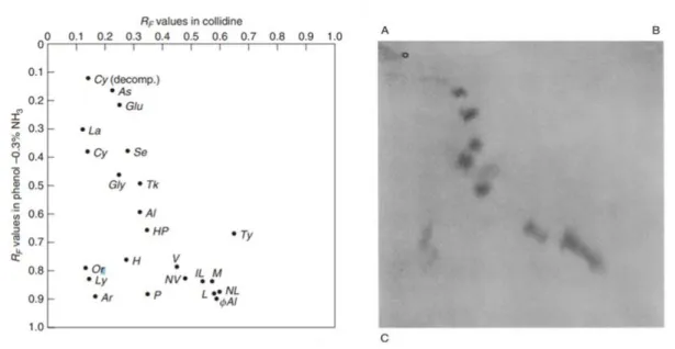
predict and to construct the “dot plots”. The expected positions of a series of amino acids on 2D chromatogram, developed by using collidine in the first dimension and a phenol-ammonia in the second dimension, is illustrated in Figure 2.10a; a good agreement between the results predicted and the experimental results can be observed in Figure 2.10b. In the latter case, the comprehensive 2D chromatogram of wool hydrolysate is shown; amino acids were first separated along the dimension A-B (1D), and then eluted along the dimension A-C (2D).
Figure 2.10. Expected positions of a series of amino-acids on a 2D paper chromatogram (on the left) and comprehensive 2D chromatogram experimentally obtained (on the right) using collidine as 1D (A-B) and a phenol-ammonia mixture in the 2D (A-C).
Pioneered by Liu and Phillips in 1991 [13] GC×GC is the most promising innovation in GC since the discovery of open-tubular columns. The leap from GC-GC to GC×GC was achieved using a special transfer device, called modulator. The latter, in a typical GC×GC experiment is located between the first and second capillary columns. In the Phillips’s paper, a GC×GC separation of a mixture of standard compounds and a sample of coal liquid was achieved by employing a dual-stage thermal desorption modulator (TDM). While the follow column combination was chosen: a capillary column (with a polyethylene glycol stationary phase) of dimensions 21 m × 0.25 mm ID × 0.25 µm df as 1D, while the 2D was
Commercially available GC×GC systems offer several features that can not be matched by 1D GC. Specifically, the main advantages of GC×GC over conventional 1D GC can be resumed in six points:
1) enhanced separation power
2) enhanced specificity (the entire sample is subjected to a separation on two chemically different stationary phases);
3) enhanced sensitivity (the chromatography band isolation process is accompanied by analyte re-concentration, especially when using cryogenic modulation);
4) enhanced identification power due to the formation of highly organized chemical class (e.g., alkanes, fatty acid methyl esters, pyrazines, etc.) patterns in the 2D chromatograms;
5) the capability to generate true sample-specific fingerprints; and
6) the generation of a higher amount of usable data per unit of time.
2.4 GC×GC: basic instrumental setup
The hardware setup of a GC×GC system (Figure 2.11) is quite simple and can be constructed using the same equipment employed for conventional 1D GC. A typical GC×GC experiment is carried out on two capillary columns (having different selectivity) connected through a sampling device, the so-called modulator. In most instances, both columns are placed in the same oven; or the second column can be housed in a different oven to enable more flexible temperature control. Thus, the only piece of hardware required to turn a 1D GC system into a GC×GC-one is the modulator. The latter can be mounted inside or outside any of the commercially available gas chromatographs. Specifically, the modulator acts as an on-line injector that produces very narrow injection pulses (down to 50 msec peak width) at the head of the second column, while respecting Giddings’s conservation rules [7]. The entire 1D chromatogram is thus ‘‘sliced’’ following a modulation period (PM) of a few seconds and re-injected into 2D for a fast GC type separation (Figure 2.11a). Ideally, the separation of analytes in the 2D has to be completed before another pulse is injected in the 2D to avoid overlap of peaks issued from different modulation cycles (an effect called “wraparound”).
Figure 2.11a-c. Scheme of the GC×GC setup. (a) The modulation process is illustrated for two overlapping compounds (X and Y) coming out from 1D at a defined first-dimension retention time (1tR). As the modulation process occurs during a defined PM, narrow bands
of sampled analytes are entering into 2D column and appear to have different second-dimension retention times (2tRY and 2tRX). (b) Raw data signal as recorded by the detector
through the entire separation process. (c) Construction of the two-dimensional contour plot from (b).
The second column analysis is much faster than the first one, thus leading to 2D separation time approximately 100 times more rapid than in the 1D. Although in principle, the detection occurs as in 1D GC, special requirements are needed for the detector used in
GC×GC, which must be characterized by
high acquisition rates,
and short rise times to accurately reconstruct the narrow chromatography bands generated. Actually, a series of high-speed secondary chromatograms of a length equal to PM (1-8 sec) are detected one after another (Figure 2.11b). They can at the end be combined to describe the elution pattern by means of a 2D plane (Figure 2.11c).Although basic information on chromatographic performance can be deduced from the modulated raw signal, a conversion process in 2D chromatogram is necessary to elaborate and visualize the overall GC×GC separation (e.g. the presence of wrap-around, the amount of occupied 2D separation space, the chemical-class pattern formation etc.). In such a respect, the use of dedicated software packages are required. The generation of a 2D plot is a simple process, each second-dimension chromatogram is stacked side-by-side and, considering the modulation time, the first and second retention times (tr1 and tr2, respectively) are derived for each peaks. The resulting planar separation space contains oval-shaped peaks (intensity is related to color), each defined by two retention time (tr1, tr2) and an area. Although not a necessity, three-dimensional plots can also be visualized, containing cone-shape peaks projected into a space defined by a z-axis.
Though building a GC×GC system may seem quite simple, GC×GC method optimization is far more complicated than that in 1D-GC.
2.4.1 Column combination
Although the modulator is considered as the key component of any GC×GC system, simply installing a modulator between two column does not guarantee an efficient GC×GC separation. As in any GC system, the selection of the most appropriate chromatographic column plays significant roles to achieve a satisfactory GC separation. In such a respect, column combination optimization, including stationary phase chemistry and column geometry, is required to accomplish efficient GC×GC separation. The main aim of any GC×GC method development is to maximize the amount of exploitable separation space, which is mainly achieved by choosing a proper columns set configuration. Following the “Giddings’s roles” [7], a successful multidimensional separation is achieved by combining two columns capable to generate an orthogonal setup. Theoretically, considering two completely-independent column selectivities and a fully-optimized separation, the peak capacity of a GC×GC system should be equal to the product of the peak capacity value relative to each column; however, such a result is an excessive estimation since both of the aforementioned conditions are never fully achieved. It must be emphasized, whatever stationary phases are used, complete orthogonality cannot be achieved because the volatility dimension will always generate a certain degree of correlation between the two separation mechanisms. For such a reason, it is not so common to observe analytes with a
low 1trvalue, and a high 2tr one (and vice versa). In fact, a high number of published GC×GC chromatograms are characterized by “fanshaped” analyte bands, with a left-to-right upward inclination, and with plenty of unexploited space. A typical example of low exploitation of the available 2D separation space can be observed in the cod oil fatty acid methyl ester (FAMEs) chromatogram, illustrated in Figure 2.12. Even though the chromatogram is well structured (C14 to C22 group-type patterns are evident), only 22.3 % of the entire 2D chromatography space is used [14]. This negative GC × GC feature can be caused by two main factors: partial correlation between the two dimensions and an excessively high second-dimension gas linear velocity. The latter aspect is discussed in depth later.
Figure 2.12. GC×GC chromatogram of cod liver oil FAMEs. Peak identification: 1.C16:0;
2. C16:1ω7; 3.C16:2ω4; 4.C16:4ω3; 5.C22:1ω9; 6. C22:6ω3.
The most common and orthogonal column configuration combines a non-polar column as first dimension, for example, dimethylpolysiloxane, and a second column with a more polar stationary phase, for example, polyethylene glycol, phenylmethylpolysiloxane, or cyclodextrine [15, 16]. In such a case, the primary-column elution order occurs according to increasing boiling points, while the secondary-column separation is dependent on
specific polarity-based interactions (H-bond, dipole-dipole interactions, dispersion forces, etc.). Any existing stationary phase that can be used in 1D GC can also be used GC×GC. A variety of stationary phases can be selected according to the intended analyte-stationary phase interaction. Many sample-types are characterized by the presence of homologous series of constituents. The GC×GC analysis of fatty acid methyl esters (FAMEs) is aperfect example to illustrate group-type order [17]. Figure 2.13 shows a complex human plasma fatty acid profile, in which homologues compounds are situated in a grid according to their chemical characteristics. In particular, saturated FAMEs are in the lower part of the 2D chromatogram, while an increase in the number of double bonds (DB) in the fatty acid chain intensifies retention in the second dimension. On the other hand, a reversed column set can better satisfy the aims of a specific research. Adahchour et al., studied and compared a normal and reversed column set for two different complex samples, namely diesel oil and food flavours [18]. When food flavour samples were analyzed, the reversed approach improved the peak shape of polar compounds, such as aliphatic acids and alcohols, which improved the ordered structure of the chromatogram. Seeley et al. used a high-temperature phosphonium ionic liquid column in a GC×GC application, proving that these phases can be considered as good candidates for the second dimension of a GC×GC setup [19]. Seeley himself introduced the concept of dual-secondary GC×GC (GC×2GC) [20]. The latter consists in the use of a dual parallel secondary column system by splitting the focused pulse towards two parallel secondary columns instead of a single one.
Figure 2.13. GC×GC analysis of human plasma fatty acids. For peak identification refer to reference [17].
Apart from the selection of the most appropriate stationary phase, the column geometry must be considered. Generally, a conventional “normal-bore” capillary column, e.g. 10-60 m, 0.25 mm ID, 0.25 µm df, is used as first dimension, while a short “micro-bore” column,
0.1mm ID, 0.1 µm df, is used as the second dimension. The secondary column generally
measures between 80 and 200 cm long to maintain elution times that are under the modulation period (i.e., 0.5-8 s) for most analytes. The direct consequence of using two capillaries with different IDs is that, under specific gas flow conditions, there will be a mismatch between the average linear gas velocity (ALV) values. In fact, it can be easily found that most GC×GC separations are carried-out at gas velocities that are ideal (or near to-ideal) in the 1D and far from optimum in the 2D. The reason for such gas velocity conditions is related to the fact that a single pressure source supplies gas to a long conventional and short micro-bore twin-column system. The most popular choice is the use of a 1D 30 m × 0.25 mm ID × 0.25 µm df capillary column followed by a segment of 1m ×
0.10 mm ID × 0.10 µm df as 2D. If a such column set is used in GC×GC-FID experiment
1.6 ml/min will be generated, corresponding to an ALV of about 30 and 265 cm/sec in the first and second dimensions, respectively. Such separation conditions are close to the ideal for a 0.25-mm ID column but far from the ideal 0.10-mm ID column (ALV to high). The GC×GC gas velocity compromise becomes less evident when the diameter of the two columns are closer. However, the proper column dimensions and column combinations, needed for a specific separation, can also be predicted by calculating the optimum flows.
2.4.2 Transfer device
As in any multidimensional system, the interface between the two dimensions is a key component in the instrumentation. The transfer device, so-called modulator, controls and sets fractions transit between the separation dimensions. Its role is to cut, possible re-concentrate, and to re-inject bands of eluate from the outlet of the primary column onto a short column segment, in a sequential, continuous way throughout the analysis. Since the transfer device is arguably considered the most important component of any GC×GC system, a deeper insight will be provided in section 2.5.
2.4.3 Detectors
The detector is another important GC×GC system component. GC×GC peak elution is normally very rapid and peak volumes small, requiring detector systems with a rather high sampling rate, limited internal volumes and a rapid rise time. All of these characteristics are necessary in order to reduce the effects of extra-column band broadening and to achieve a proper peak reconstruction (10 points per peaks are sufficient in the most cases). A brief discussion about detectors employed in GC×GC follows.
Flame ionization detector. The most commonly employed detector in GC×GC is the flame ionization detector (FID), which is capable to operate under very high sampling frequency
conditions, easily above 100 Hz. It operates on thebasis of decomposing the solute-neutral molecules in a flame into charged species and electrically measuring the resultant changes of conductivity. A cross-sectional view of a flame-ionization detector is shown in Figure
2.14. A small flame is sustained at the jet tip by a steady stream of pure hydrogen, while
the necessary air (oxidant) is supplied through the diffuser. At the detector base, the column effluent is continuously introduced, mixed with hydrogen, and passed into the flame.
Conductivity changes between the electrodes are monitored, electronically amplified, and recorded. A conventional carrier gas contributes little to the flame conductivity; however, when organic solute molecules enter the flame, they are rapidly ionized, increasing the current in accordance with the solute concentration. With most flame-ionization detectors, this current increase is linear with the solute concentration up to six orders of magnitude. The flame-ionization detector is a carbon counter; each carbon atom in the solute molecule that is capable of hydrogenation is believed to contribute to the signal (compounds with C—C and C—H bonds), while the presence of nitrogen, oxygen, sulfur, and halogen atoms tends to reduce the response. The detector is most sensitive for hydrocarbons. Practically, no response is obtained for inorganic gases, carbon monoxide, carbon dioxide, and water. With such a detector, group-type 2D chromatograms can be obtained, and tentative peak classification can be achieved. The group type is assigned according to retention time correspondence with even one standard, and then FID quantification can easily be done. Biedermann and Grob exploited GC×GC-FID for the quantification of mineral oil constituents contained in a contaminated sunflower oil [21]. GC×GC-FID has been employed in several fields, such as environmental [22, 23], industrial [24], and food [25, 26]. The main drawback of using an FID, is the lack of structural information.
Figure 2.14. Schematic diagram of a flame ionization detector (A) and a co-axial cylinder electron-capture detector (B).
A variety of different other detectors have been used in the GC×GC field. The electron
capture detector (ECD) is a concentration-dependent device and is characterized by a high
specificity for organic molecules containing electronegative functional groups (halogens, phosphorous and nitro-groups). The main concern in coupling such a detector, has been related to a rather high internal volume, which can cause band broadening. The atomic
emission detector (AED) is a device capable of measuring up to 23 elements: a He plasma
chamber receives the GC effluent, and due to the high temperature encountered therein, the analytes are decomposed to their constituent atoms. Van Stee et al. reported the use of a GC × GC -AED system in petrochemical and pesticide applications [27].The thermionic
ionization detector (TID) is often used for the selective detection of N and P-containing
compounds (in this case, it is also defined as the nitrogen phosphorous detector-NPD) and is structurally similar to the FID, apart from the presence of a ceramic bead doped with an alkali metal salt, located above the jet. Engel et al. reported the optimization and evaluation of a GC × GC –TID method for pesticides analyses [28]. The helium ionization detector (HID) is a sensitive and universal detector, used in particular for compounds with no or a limited FID response. The HID has been used only rarely in the comprehensive 2D GC field; the first application was reported by Winniford et al., who used a miniaturized pulsed discharge HID, in cryogenic-modulation (CM) GC × GC applications [29].
A discussion apart has to be made on mass spectrometers, the most informative detection systems, considered as an additional third dimension analysis by GC×GC users. The use of mass spectrometry (MS), as GC×GC detector dates back over 20 years ago [30], when Frysinger and Gaines reported the use of a single quadrupole mass spectrometer (QMS) system with a very low acquisition speed (2.43 scan s-1). More detailed descriptions related to the use of GC×GC-MS systems in the field of food analysis, are reported in the following
Chapters.
2.5 Modulators
As the “heart” of a GC×GC system, the modulator is located between the 1D and the 2D column, acting as an online injector that produces very narrow injection pluses onto the 2D, generating fast secondary separations. Each modulator operates on the premise of sampling, focusing, and reinjecting portions of the 1D effluent onto the head of the 2D column, facilitating a comprehensive separation. The simply serial connection of two different
columns without a modulator between them, does not achieve a GC×GC separation. Figure
2.15 explains the need for and the role of the modulator. Specifically, panels A-C in Figure 2.15. illustrates a separation with no modulator between the two columns, which
essentially, will result in one-dimensional separation. In addition, there is also the possibility of the changing the elution order of the analytes due to different selectivity of the 2D column (Figure 2.15-C). Differently, panels D-G illustrates a separation when the modulator interfaces the two columns. The analytes which are approaching the modulator interface (Figure 2.15-D) are collected or sampled for a designed period of time (according to PM) (black in Figure 2.15-E). They are then re-injected as a narrow pulse onto the head of the 2D column. In the meantime, the following chromatographic band is sampled (Figure
2.15-F). Focusing and re-injection of this analyte band allows for further separation in the
2D only after the previous band had eluted from it. In the meantime the last analyte band
eluting from 1D is collected by the modulator (Figure 2.15-G).
Figure 2.15. The relevance of the modulator in GC×GC. A-C illustrate how bands separated on one column can recombine or change elution order on the second column if they flow uncontrolled from one to the other. D-G illustrate how the interface traps material from the primary column, and then allows discrete bands to pass to the second dimension column while trapping other fractions.
Various technological improvements have been made throughout the development of modulators and they can be broadly classified in two categories: thermal and valve-based, or flow, modulators. Another general distinction exists between one- and dual-stage modulators: in the latter, two events in series occur in two different zones of the modulator.
Thermal modulators can be further divided in two different classes, namely cryogen-based
and cryogen-free modulators. While among valve-based modulators, two more approaches can be identified, namely those which employ a differential flow modulation, and those employ a flow diversion modulation.
2.5.1 Thermal modulators
The term “thermal modulator” is employed for any devices that use a positive and/or negative temperature, compared to the GC-oven temperature, to achieve a GC×GC separation. It relies on low temperatures to trap and focus analytes exiting from the 1D column and re-inject them onto the 2D column through rapid heating. Based on the various designs, the trapping stage can be accomplished using a thick stationary phase film, intense cooling, or combination of the two. The main advantage of thermal modulation over flow modulation is the focusing effect from the re-concentration of the analyte bands during trapping, thus leading to an enhancement of the signal-to-noise (S/N) ratio. In the pioneering GC×GC design, analytes eluting from 1D were transferred onto the 2D using a thermal modulator, namely a thermal desorption modulator (TDM). The latter, was originally developed as a sample introduction device in multiplex and high-speed gas chromatography [31-34]. It was only in 1991 [35] that Liu and Phillips, used the TDM to perform the first dual-stage modulated GC×GC separation. A dual-stage modulation was achieved by alternating two events during the entire analysis; a trapping stage based on phase-ratio focusing; and a re-injection one accomplished by thermal desorption. A scheme of TDM-GC×GC system proposed by Phillips is below reported, Figure 2.16. The TDM interface was constructed by coating the initial part of the secondary column with a film of electrically conductive material, namely gold paint, and by looping it outside the GC oven, at room temperature. The modulator was 15 cm in length, divided equally between two stages.
Figure 2.16. Scheme of TDM-GC×GC-FID system employed by Liu et al. [35]. An expansion of the modulator is shown in the bottom part.
The principal of its operation is shown in Figure 2.17 and it consists on the following steps:
(1) analytes eluting from the 1D column were entrapped in the thick film of stationary phase outside the GC oven (band compression I), at ambient temperature (step 1a);
(2) the application of an electrical pulse to the conductive capillary tube resulted in heating of the stationary phase and drove the analytes back into the gas phase, thus leading to their re-mobilization ending the first modulation stage (step 1b);
(3) the re-mobilized fraction, transported by the carrier gas, reach the second “cold” segment of the modulator (band compression II);
(4) another narrow chromatography plug begins to be accumulate at the modulator head, which has rapidly cooled down to ambient temperature (step 2a);
(5) at this point, another electrical pulse is directed to the second modulator segment, launching the narrow band onto the secondary column (step 2b), thus ending the second modulation stage
Figure 2.17. Dual-stage thermal desorption-modulation process on two compounds, co-eluting in first dimension.
(6) the different secondary-column selectivity will enable the delivery of two separated compounds to the detector; and
(7) 2 s the first electrical pulse, the next modulation process was initiated.
Although successful in accomplishing the first GC×GC separation, the design was not very robust due to frequent burnouts and the delicate nature of the thin conductive films. Many efforts have been made on the designs of thermal modulator over the years, and today they can be further broken down into two subcategories: cryogen-based, and cryogen-free modulator, which are often further divided into movable and static modulators, respectively.
2.5.1.1 Cryogen-based modulators
Cryogen-based modulators use cryogens to provide cooling in order to trap the solutes at temperatures significantly lower than the oven temperature. The re-mobilization step is achieved once that the cooled section of the modulator is brought back to or higher than the GC oven temperature. Although the use of cryogens (LN2 or CO2) for thermal modulation added a consumable cost to the system, it remains popular and continues to be further developed.
Longitudinal movement design. Cryogen-based modulation was first described in 1998
[36] when Kinghorn and Marriott reported the use and the basic principles of the
longitudinally modulated cryogenic system (LMCS). A schematic representation of the
LMCS device can be displayed as in Figure 2.18. The end part of a 30 m×0.22 mm ID×0.25-μm df non-polar capillary column was linked to a movable 5-cm cryo-trap which
entrapped/focused effluent fractions by means of an internal CO2 flow which generated intense cooling. The longitudinally motion of the CO2-cooled cryo-trap towards two different position (marked as “R” and “T”) along the head of the second dimension, allowed the modulation process. Specifically, analytes exiting from the first dimension were cold-trapped in a small region of the column (position marked as “R”). In the following step, the cooled spot of the column was exposed to the GC oven temperature via the longitudinal motion of the trap to the downstream region (position marked as “T”) of the column. The desorbed band, transported by carrier gas flow, were moved along the column to be subject to a second trapping stage in the bottom segment (“T”). The motion of the cryo-trap back its original position, “R”, allowed the trapped analytes to be re-injected onto the secondary column, while preventing any potential analyte breakthrough.
Figure 2.18. Device for longitudinally modulated cryogenic system (LMCS). Analytes are sampling when the trap is in the T position, and re-injected when the trap reach the R position.
The longitudinal motion of the trap was driven by a pneumatic, electrical, or stepper motor actuator through a modulator arm connected to the trap. The LMCS offered significant advantages over the thermal sweeper: i) more efficient entrapment, owing to the low trapping temperature; ii) no GC-oven-temperature limitation, except that related to the less thermally-stable stationary phase employed; and, ii) less elaborate construction. On the other hand, there were some limitations to this approach. The first was the consumption of liquid CO2 employed as a cryogenic agent, boosting the cost/analysis. Another limitation was the use of a moving trap, which could damage the column or cause other problems.
Static jets design. The moving parts were eliminated from the design of CMs when Ledford
et.al. [37] described a dual stage static modulator, namely quad-jet modulator. As shown in Figure 2.19, this modulator used two hot jets and two cold jets situated at the head of the second column, to achieve a dual stage modulation. These jets were positioned to provide a transverse gas flow onto the head of the second column and were pulsed in an alternative mode.