Deep learning techniques for Intelligent Cyber Physical Systems: towards a new generation of smart and autonomous things

(1)

Universit`

a degli Studi di Messina

Department of Engineering

Doctoral Programme in Cyber Physical Systems

XXXIII Cycle

Deep Learning Techniques for Intelligent Cyber

Physical Systems: Towards a New Generation of

Smart and Autonomous Things

Student:

Fabrizio De Vita

Advisor:

Prof. Dario Bruneo

Co-Advisor:

Prof. Sajal K. Das

(2)

Abstract

We are living an era constantly surrounded by objects blended with the envi-ronment. During the last decade, the advent of the Internet of Things totally revolutionized the way we interact with these objects, and acted as a catalyzer for the creation of a wide variety of Cyber Physical Systems exposing services to support the human being under different aspects of his life. Today, the maximum expression of Cyber Physical Systems are smart environments whose task is to simplify (or automate) certain types of operations to help their “guests” during the daily activities. Cloud and Edge computing paradigms play a fundamen-tal role for the realization of these systems; the first providing storage and high performance computing capabilities, the second allowing a pervasive monitoring and an early processing of the data gathered from sensors. In such a context, Artificial Intelligence is another very important player which gained a lot of in-terest during these years, thanks also to the advancement in ICT and the huge amount of available data. Leveraging the above mentioned technologies, it allows the implementation of a new type of intelligent systems (e.g., Intelligent Cyber Physical Systems) able to make “reasonings” and perform autonomous actions according to the context. This thesis work presents a deep study of all these technologies and proposes intelligent systems and algorithms solutions applied to several fields (i.e., smart home, smart city, smart industry, smart health, and smart agriculture) focusing also on the challenges emerged during the design and implementation processes. Experimental results demonstrate the feasibility of the proposed approaches and show the benefits derived from using them.

(6)

Introduction

The progresses made in ICT technology during the last decade allowed the con-struction of a network that enables the interaction with objects. We usually refer to this phenomenon with the term Internet of Things (IoT) to indicate the trend where common use objects are equipped with an “intelligence” and act as sensors and actuators [1]. The advent of IoT totally revolutionized the way we interact with the physical world, in such a context, objects become an active compo-nent of the environment, and because these systems usually expose an interface also with the cybernetic world, they are usually called Cyber Physical Systems (CPS) [2]. CPS are a new generation of devices exhibiting advanced functionali-ties. Thanks to their multiple ways to interact with the human being and their computation capabilities strictly related to the physical world, they represent an enabling technology for the future systems development [3].

Today, smart environments represent the maximum expression of CPS; here, fleets of objects are connected together acting as bridges to the physical world and exposing several services to support their inhabitants. Originally intended to ease the life of the human being, today the market related to this technology expanded very quickly producing specialized solutions. Smart industry, smart cities, smart health, etc. are just a few examples which demonstrate the wide range of available applications that allow to enhance the productivity and the effectiveness of a system. In such a context, the Cloud plays a key role pro-viding storage and computing capabilities to perform complex operations (e.g., data analysis, execution of onerous algorithms, etc.). Moreover, the Cloud can

(7)

INTRODUCTION

be seen as an “orchestrator” that manages and coordinates all the components of an environment. Although the Cloud paradigm is useful to realize these sys-tems, the advent of CPS and IoT gave the birth to new types of services and applications which pose significant challenges that the Cloud is usually unable to handle. For example, when working with applications with low latency or real time requirements, the use of the Cloud paradigm becomes unsuitable. Analogue is the condition for those services containing sensible data that should not travel the Internet.

The above mentioned examples, are just two of the many conditions where the Cloud becomes ineffective, thus leading to a new paradigm where the computation is shifted “closer” to the data [4]. This paradigm is called Edge computing and indicates a model where the computation is done directly on the device (e.g., an embedded system, a smartphone, a smartwatch, etc.) which generated the data or very close to it. However, the constrained resources of Edge devices make them suitable to perform simple operations. In this sense, the shift of computation from the Cloud to the Edge is not easy and requires a careful design of applications and services that can effectively run of these devices. Nowadays, modern systems exploit both the paradigms building hybrid platforms, where data is usually collected and preprocessed on the Edge and then sent to the Cloud to store it and perform more complex analysis.

Artificial Intelligence (AI) is another important player for the implementation of intelligent applications. Born in the 80’s, this promising technique has always faced the problem related to the data gathering which slowed down its growth. Today, this problem has been largely solved thanks to the IoT widespreading that acted as catalyzer for the generation of a huge amount of information. AI brings the applications and services to a whole new level providing an advanced data processing, and becoming an active element in the decision process during the execution of a task. Through machine learning and deep learning in fact, it is possible to build new types of systems equipped with a layer of intelligence

(8)

INTRODUCTION

that helps them to make context aware decision autonomously [5], and for this reason called Intelligent Cyber Physical Systems (ICPS). Such systems (in com-bination with Cloud and Edge paradigms) represent the core elements of modern frameworks and are used as entities capable to deliver a “reasoned” support to the human being during his daily activities.

Leveraging the above described technologies, this thesis work presents the study, design, and implementation of machine and deep learning solutions for ICPS on several smart application contexts (i.e., home, city, industry, health and agriculture). Starting from the problem analysis, we present the literature overview to describe the current state of the art and compare it with our tech-niques. In such a context, we provide a detailed description of the proposed solutions putting in evidence the challenges we faced during their realization. We also prove the effectiveness and feasibility of the proposed systems through the experimental results, highlighting the benefits derived from their implementation. The rest of the thesis is organized as follows. Chapter 1 provides a back-ground on ICPS, machine and deep learning technologies which are at the base of this thesis work. Chapter 2 presents an indoor localization system that ex-ploits deep learning and wireless fingerprints to locate the user inside a smart environment. Chapter 3 proposes two different solutions to improve the overall performance of applications executed in smart city scenarios. Chapter 4 focuses on the realization of smart industry solutions that allow to monitor, detect, and prevent the occurrence of faults in industrial plants. Chapter 5 presents a smart health technique that uses wearable computing and deep learning techniques to create a support system for the prevention of pressure ulcers formation. Chapter 6 describes an ICPS solution for smart agriculture running on the smart Edge to assess the health conditions of plants. Finally, Chapter 7 concludes this thesis work and gives a vision of the steps necessary to extend the AI to a human level.

(9)

Chapter 1 Background

ICPS totally revolutionized the way we interact with the physical world; together with machine learning, they paved the way for new types of intelligent applica-tions which exhibit cognitive capabilities improving our quality of life. In this chapter, we provide a general background of these two technologies which are at the base of this thesis work.

1.1 Intelligent Cyber Physical Systems

ICPS represent a very important resource for the fourth industrial revolution. Wanting to give a definition, ICPS are computer systems (usually blended with the environment) that allow to integrate sensing, actuating, and computing func-tionalities into the physical world and exposing, among other things, Internet communication capabilities [3]. The combination of physical processes with the computation is not new. Embedded systems are a perfect example of this trend, however, they are usually “closed” towards the external world and do not ex-pose their computing capabilities [2]. In this sense, thanks to their possibility to interact with the cyber and the physical worlds, ICPS provide a pervasive infrastructure that can support the human being in many different ways [6]. In the recent period, a growing interest has arisen towards this technology, dictated

(10)

CHAPTER 1. BACKGROUND

by the desire to equip these systems with such an “intelligence” to make them autonomous, and capable of taking decisions. In such a context, AI plays a deci-sive role in bringing the intelligence on CPS. Thanks to machine learning in fact, we introduce a “cognition” layer that enables a system to learn a task exploit-ing its ability to sense the physical world. Figure 1.1 depicts a typical scenario where the ICPS act as a connecting bridge exposing a double interface to put in communication the cyber and the physical worlds. Here the sensing/actuating layer is the closest to objects and, as the name suggests, it is responsible to sense the environment and interact with it via a set of actuators (e.g., switches, mo-tors, etc.). The computing layer on the other hand has the task to process the data coming from both the two worlds and works in synergy with the cognition layer added via AI techniques. In this sense, ICPS exhibit a context awareness of the surrounding environment that results fundamental for the delivery of tailored services. Sensing/Actuating layer Computing layer Cognition layer Sensors Things Physical world ICPS Cyber world

(11)

ICPS completely revolutionized the way we interact with things, however they also pose significant challenges most of which related to the pervasive nature of this technology. In particular, the uncertainty of the environments requires the design of robust and fault tolerant systems in order to face unpredictable conditions that can compromise their operation [7]. Security should be another concern during the realization of an ICPS. Their capability to have a direct access to the “physical reality” imposes the implementation of mechanisms to prevent and contrast possible external attacks. A careful networking management is also necessary to provide a good quality of service, in this sense ICPS should exhibit self-organizing techniques to guarantee their autonomy [7]. Of course, some of these problems are not new, but they should be analyzed under a different perspective in order to propose effective solutions.

Despite the above mentioned challenges, today ICPS have a wide range of applications scenarios where their usage allows to improve the overall systems quality, productivity, and effectiveness.

1.2 Machine learning

In the introduction and in the previous paragraph, we mentioned that ICPS are equipped with an intelligence provided by machine learning, but we did not provide a proper definition of this technique. Machine learning is a branch of AI that gives, according to Arthur Samuel, to a computer or a device “the ability to learn without being explicitly programmed ”. The base idea of this technique consists in the definition of a mathematical model that is able to fit the output of a function which is not known a priori. Depending on the nature of this output, it is possible to split the machine learning problems into two categories, namely: regression and classification problems [8].

In general, we talk about regression problems when the output we want to predict is a continuous value (e.g., a temperature, a price, etc.). In such a context,

(12)

statistical modeling provides the so called regression analysis through which is possible to determine the relationship between the dependent variables (i.e., the outputs) and the independent variables (i.e., the inputs) called features. Given a regression problem, we can define the following quantities: the features vector X, the outputs vector Y , and the vector of parameters θ which is not known. The relationship which binds these quantities can be defined as follows:

Y = f (X, θ), (1.1)

where f (.) is a function not known a priori. In such a context, the task of machine learning is to find the best set of parameters θ such that the difference:

Y − bY , (1.2)

(where bY is the value estimated by the model) is minimum.

With respect to classification, we refer to this problem when the output to predict is a discrete value (e.g., digits from 0 to 9, cancer type, etc.). In this sense, the task of a machine learning classifier is to determine the most fitting category (i.e., the class) for a given feature vector X. Likewise for the regression, the algorithm has to find the best set of parameters θ such that a score function:

score = f (X, θ), (1.3)

returns the most probable class associated to X according to the score.

Depending on the data and the task to accomplish, machine learning prob-lems can be further split into three categories: supervised learning, unsupervised learning, and reinforcement learning [8].

Supervised learning

In supervised learning problems the machine learning model is provided with a set of inputs and the corresponding outputs (i.e., the labels). The term supervised

(13)

comes in fact from the “supervision” of the human being, who provides to the model a feedback of the real world that is exploited to fit the data. In general, during the implementation of a supervised machine learning algorithm we can identify 5 main steps, namely: dataset construction, algorithm choice, model selection, model training, and model testing [8].

The first step is probably the most important one. During this phase in fact, the data is collected, organized, and the inputs and outputs of the problem are defined. The importance of this step comes also from the quantity and the quality of the collected data that determine the quality of the machine learning model. Once the data is collected, the next step is the choice of the most suitable algorithm. This process can be executed in different ways, but most of them imply the use of empirical trials. Since a lot of machine learning models require a manual setup, the model selection (or model validation) step is necessary to select the best set of input parameters (or hyperparameters). The fourth step is based on the training of the selected model. Of course this phase changes according to the algorithm, however, its goal is always to fit the input data while minimizing a cost function (usually denoted with J ). In such a context, since we talk about supervised learning problems, the model can use the labels as an indicator that helps to understand if it is learning or not.

The last step is the model testing. This phase is necessary to test the “gener-alization” capabilities of the model on a new set of input data that it has never seen (i.e., not belonging to the training data). Unlike the training step, during this phase the model is only fed with the input without the corresponding labels that, in this case are used to test the learning. In this sense, if the model is able to correctly predict the output labels with a good level of accuracy, then this means it acquired the generalization capabilities necessary to “learn” the task.

(14)

Unsupervised learning

Unsupervised learning is a class of machine learning problems characterized by the absence of labeled data. Likewise the supervised, also in this case the imple-mentation of an unsupervised algorithm is done performing the above described steps. However, this kind of learning is in general more difficult if compared to the supervised one because of the absence of a feedback. Nevertheless, this technique is very useful for a wide variety of machine learning tasks especially related to clustering problems, whose goal is to group inputs with similar patterns or struc-tures. In general, unsupervised learning is very helpful also as a preprocessing step for the data organization or visualization before passing it to a supervised algorithm.

Reinforcement learning

Reinforcement Learning (RL) is a machine learning technique used to observe an environment and learn an optimal policy with respect to one or more performance indexes. From a structural point of view, RL is very similar to the supervised learning, with the only difference that, in this case, a reward is used instead of the labels. It adopts as base formalism a Markov Decision Process (MDP) that allows to model a decision process in a stochastic environment. From a mathematical point of view, a MDP is defined through a set of states S that the environment can assume, a set of actions A that can be performed in the environment, a reward function R(s) : S → R which defines the reward associated to an action, and a discount factor γ ∈ [0, 1] stating the importance of future rewards. The objective of RL is to use an entity called agent to find an optimal policy that maximizes the reward on an environment. To do that, it builds a trial and error process by making actions while traversing the states inside the environment several times, and changing the learned policy according to the feedback received from the rewards. A typical RL approach is the Q-learning [9] a model-free technique based on the use of the Q-values Q(s, a) to learn an optimal policy in

(15)

an environment. A Q-value is a real number representing the utility of doing the action a while the agent lies on state s; these values evolve as the agent takes action in the environment according to the following equation:

Q(s, a) = Q(s, a) + α · (R(s) + γ · maxa0Q(s0, a0) − Q(s, a)), (1.4)

where α is the learning rate, R(s) is the reward function, γ is the discount factor, s0 is the state towards which the environment will evolve by taking action a, and

a0 is the action to which corresponds the highest utility (i.e., the highest Q-value) when in state s0.

RL finds a large application especially in optimal control problems where an agent is trained to learn a policy on a given environment.

1.2.1 Artificial Neural Networks

Artificial Neural Networks (ANNs) are a family of non-linear function approxima-tion algorithms inspired by the biological brain [10]. From an architectural point of view, ANNs are systems of interconnected components (called neurons) which are able to process data [10]. Each connection is characterized by a weight (like in a weighted graph), and to each neuron is associated a bias (typically a constant value) whose task is to increase the model flexibility by shifting its output.

Figure 1.2 depicts the simplest possible ANN (consisting of one neuron) which takes the name of perceptron. From a mathematical point of view the operation executed by a neuron is the following:

y = f ( n X

i=1

xiwi+ b), (1.5)

where y is the output of the neuron, xi is the i − th input, wi is the weight

asso-ciated to the i − th input connection, and b is the neuron bias. Before generating the output, the result of the above defined summation passes through a function f (.) called activation function. Such a function plays a very important role since

(16)

Inputs

x

₁

x

₂

. . .

x

_n

_b

w

₁

w

₂

w

n

∑

f

y

Output

Figure 1.2: Structure of the perceptron.

it strongly affects the output of the neuron and enables ANNs to learn non-linear relationships between the input and the output. Table 1.1 shows some of the most popular activation functions used in modern ANNs applications i.e., the Sigmoid, hyperbolic tangent (tanh), Rectified Linear Unit (ReLU), Leaky ReLU, and Expo-nential Linear Unit (ELU). Each of these functions introduces a non-linearity to the ANNs which can produce very different results. In this sense, they require a careful usage and a deep understanding of the machine learning problem. Unfor-tunately, the single perceptron is not able to learn complex relationships between the input and the output, for this reason it is usually organized in structures called layers that group a set of neurons to perform advanced calculations.

Today, the most common topology in ANNs is the multilayer perceptron (or feedforward ANN ) (showed in Figure 1.3) whose structure is characterized by the connection in cascade of multiple layers of perceptrons (called hidden layers) between the input and the output. In such a context, the main goal of the ANN is to find the best set of parameters for each network neuron (i.e., the weights) such that the error function J is minimized.

To do that, ANNs use a supervised technique which is a combination of two algorithms, namely: backpropagation, and an optimizer to iteratively update the weights values. The first one, it is responsible for the gradients computation of

(17)

Input layer Hidden layer Output layer

Figure 1.3: Example of a multilayer perceptron topology.

the error function with respect to the network parameters of the ANN (denoted with θ). In particular the term backpropagation derives from the fact that error gradients are back propagated from the output layer to the input one [11] via the chain rule, a technique used in calculus to compute the derivative of composite functions. In this sense, the computation of the error derivative returns useful information that can be exploited to have an understanding on how the network parameters should change in order to reduce the cost function effectively. On the other hand, the optimizer algorithm has the task to compute and update the ANN weights given the error gradients, thus performing the actual “learning” process [11]. For a better understanding in the following equation

wnew_i,j = wold_i,j − α · ∂J ∂wi,j

, (1.6)

we report an example of a weight update where wnew

i,j is the new generic weight computed by the optimizer, wold

i,j is the old weight at the previous iteration, ∂w∂Ji,j is the error gradient with respect to the weight value computed via backpropagation,

(18)

and α (denoted sometimes also with η) is the learning rate defining the magnitude of the optimization step.

Table 1.1: Main activation functions.

Name Graph Function

Sigmoid y = 1 (1+e−x₎ tanh y = tanh (x) ReLU y =    x x ≥ 0 0 x < 0 Leaky ReLU y =    x x ≥ 0 ax x < 0 ELU y =    x x ≥ 0 a(ex_{− 1) x < 0}

Wanting to synthesize the learning process of a feedforward ANN, it consists of the following 4 steps: forward pass, error computation, gradient computation, and parameters update. In the first step, the data is forwarded from the input to the output layer for the ANN output computation. If we consider a traditional ANN, this task is accomplished by repeating multiple times eq. (1.5) according to the model topology. In the second step, the network computes the error; since

(19)

the algorithm is supervised, this can be done comparing the output produced by the ANN in the forward step and the corresponding ground truth label. In particular to make the comparison, ANNs use very specific cost functions from which is possible to effectively compute informative gradients. Functions like: Mean Squared Error (MSE), categorical cross-entropy, binary loss, etc. today are at the base of the learning process of many machine learning applications. Finally, the last two steps are executed via the above explained backpropagation and optimization algorithms. It is worth to mention that the learning (or training) of an ANN is an iterative process, which means that these steps are continuously repeated until a stop condition is satisfied.

1.2.2 Deep learning

Most of the core concepts of deep learning were defined between the 80’s and the 90’s. The idea that a machine can “think” is even older, however, only in the recent period we assisted to its wide spreading. The reasons for such a diffusion are twofold: i.) a massive availability of labeled data (thanks to IoT and CPS); ii.) the improvement of hardware capabilities that enabled the execution of onerous algorithms.

Deep learning is a subclass of machine learning algorithms that uses several layers (composed by non-linear processing units) connected in cascade, to discover intricate relationships between the input parameters (i.e., the features) and select the most useful by means of the so called features extraction process [12]. Such a process, given a set of input features is able to detect (and virtually remove) those ones which are redundant or not informative. Today, deep leaning and more specifically Deep Neural Networks (DNNs) find a lot of applications in different fields (e.g., computer vision, speech recognition, natural language processing, etc.). From a topological point of view, a DNN is an ANN with a larger number of hidden layers (in general more than two) between the input layer and the output one. DNNs are able to learn complex non-linear relationships between

(20)

the input and the output, however, they make harder the training phase because they require:

• a higher number of samples for the training; • a careful tuning to avoid data overfitting; • more computation time.

Typical DNNs are Recurrent Neural Networks and Convolutional Neural Net-works that will be explained in the next paragraphs.

Recurrent Neural Networks

Recurrent Neural Networks (RNNs) are a family of neural networks particularly suitable for the processing of sequences of data [11]. The base idea to pass from a traditional DNN to a RNN is the use of a self loop (as showed in Figure 1.4) that allows to maintain the information coming from the “past”, thus enabling a memory mechanism known as hidden state.

Unfold ht ot xt ot−1 ot ot+1 x_t₋₁ xt xt+1 ht−2 ht−1 ht ht+1 Figure 1.4: RNN neuron.

Considering a sequence xtwhere t represents the time step at which is received,

the hidden state of the RNN at the time step t is a function of the current input, the network parameters θ, and the previous hidden state at the t − 1 time step:

(21)

where f (.) is the activation function (see Table 1.1) [11]. In the same way, we can define the output at the t time step ot as:

ot= f (ht), (1.8)

where f (.) is the activation function of the output layer. When working with RNNs we can think to “unfold” them over time to have a better vision of what is happening internally. Starting from eq. (1.7) and reorganizing it in order to make explicit the hidden state, we obtain:

ht= f (xt, f (xt−1, f (xt−2, ..., f (x1, h0; θ); θ); θ); θ), (1.9)

where we can notice the inner relationship that binds the different time steps. In this sense, the output at the time instant t (see eq. (1.8)) is also “affected” by the past values of the state which explains why RNNs are suitable for ma-chine learning tasks where the input order or time are crucial (e.g., in speech recognition).

Unfortunately, RNNs suffer from the so called vanishing gradient and gradient exploding problems especially when the number of unfolded time steps is large [13], [14]. In particular these conditions derive from eqs. (1.8), (1.9) where emerges a product of many factors when computing the error gradients. In this sense, the algorithm back propagates the gradients through the unfolded RNN navigating “back in time” and for this reason is called backpropagation through time (BPTT). In such a context, if we consider an unfolded RNN of t time steps (with large t), the gradient takes the form of a product of the same quantity:

∂J

∂θ = θ · θ · ... · θ. (1.10)

According to math, if θ parameters are > 1, then the derivative value will tend to exponentially increase (as long as the RNN goes deep) reaching the in-finity in certain cases, thus causing the gradient explosion. On the other hand,

(22)

if θ parameters are small (i.e., < 1) the gradient value will tend to exponentially decrease as long as the time steps increase, until its vanishing. Both these prob-lems pose significant challenges during the RNNs implementation and require a careful design of their topologies in order to avoid these issues during the training process.

Convolutional Neural Networks

Convolutional Neural Networks (CNNs) are a class of DNNs mainly used in image and visual recognition tasks. From an architectural point of view, a CNN is very similar to a traditional feedforward DNN, in this sense, the main difference that characterizes this kind of networks are two specific layers i.e., the convolution and the pooling (as showed in Figure 1.5).

Figure 1.5: Example of a Convolutional Neural Network.

In particular, the purpose of the convolution layer is to perform a feature extraction process on the image passed as input, while maintaining the “spatial” relationship between the pixels. From a CNN point of view, the convolution step consists in a linear operation between two matrices (usually called input and kernel ) that produces in output a feature map as depicted in Figure 1.6 [11]. In such a context, the kernel slides over the rows and columns of the input matrix and computes the feature map as follows:

(23)

CHAPTER 1. BACKGROUND a b c d e f g h i j k l w x y z

Input matrix Kernel matrix

aw+bx + ey+fz bw+cx + fy+gz cw+dx + gy+hz ew+fx + iy+jz fw+gx + jy+kz gw+hx + ky+lz Feature map

Figure 1.6: Convolution operation.

Fi,j = X h X w I(i + h, j + w)K(h, w), (1.11)

where Fi,j is the generic element of the feature map, h is the number of kernel

rows (i.e., the height of the kernel), w is the number of kernel columns (i.e., the width of the kernel), i is the row index, and j is column index. The output of this operation is a new matrix (i.e., the feature map) whose dimensions can be computed starting from the ones of the input and kernel matrices [15]:

Fh =

Ih− Kh + 2P Sh

+ 1, (1.12)

where Fh is the feature map height, Ih is the input matrix height (i.e., the number

of rows), and Kh is the kernel height (i.e., the number of rows of the kernel). With respect to P , it is representative for the padding option which consists in adding a zero padding around the input matrix in order to preserve its dimensions after the convolution step. Finally, the Sh term defines the stride with respect to the

(24)

input matrix during the convolution step. Likewise we did for the height, we can compute the width of the feature map as follows:

Fw =

Iw − Kw+ 2P Sw

+ 1, (1.13)

where the parameters are exactly the same we already described in eq. (1.12), but this time referred to the input and kernel widths and columns.

Typically in CNNs, after the convolution step, we apply a non-linear activation function that helps the network to learn possible non-linear relationships between the input and the output. Such an operation is then followed by a pooling step whose task is to further modify the output of the convolution [11]. Pooling operations play a very important role in CNNs since they allow to reduce the network feature space, thus simplifying the overall model complexity. Specifically, this operation replaces the output of a CNN in a certain spatial location with a value derived from the “nearby” outputs [11]. Examples of typical pooling operations are: max-pooling and average-pooling where the values of the feature map falling inside a rectangular area are respectively replaced with the maximum and the average values. For a better understanding, in Figure 1.7 we report an example of max-pooling where we considered a pooling window with height and weight set to 2.

Likewise the convolution, the pooling step is performed by sliding the pooling window through the feature map rows and columns and generating a new matrix whose dimensions are computed in the same way we did in eqs. 1.12, 1.13. In all cases, the pooling operation allows to make the feature map invariant to small variations of the input. Such a functionality is very helpful for example, when we are interested in knowing the presence of a feature inside an image instead of its precise location and provides a higher “elasticity” to the CNN model during the prediction task [11].

By looking at their architectures, CNNs topologies consist of two parts: a first one where a sequence of convolution and pooling operations are performed to

(25)

CHAPTER 1. BACKGROUND 28 1 2 21 15 7 3 27 92 50 10 96 28 7 27 92 50 96

Figure 1.7: Max-Pooling operation.

extract informative patterns from the input images through the feature extraction process we described. The second one is a multilayer perceptron network that receives in input the features preprocessed by the first part of the network and performs the actual visual recognition task.

(26)

Chapter 2 Smart Home

Smart home is the most common example of smart environment. Thanks to a wide variety of consumer products available in the market, today the home automation has become a reality accessible to everyone. In such a context con-stellated by objects emerges the necessity to locate the user to deliver a better and more precise interaction with the environment. Unfortunately, the use of the GPS technology is not possible for indoor localization due to strong signals at-tenuation. In this chapter, we face this problem through the exploitation of deep learning techniques and radio fingerprints coming from a set of wireless access points [16].

2.1 Indoor user localization

Wireless technology wide spreading together with mobile computing devices and IoT generated the interest in the development of Location Based Services (LSBs) whose market is expanding [17]. Such services, are becoming a very important part of our lives and represent the core elements for the implementation of smart applications which are strictly related to the position of the user in an environ-ment.

(27)

CHAPTER 2. SMART HOME

a set of operations which can be partially or fully autonomous; to do that, a smart environment should exhibit a context-awareness capability in order to understand its current state (by means of several sets of sensors) and determine which action should be executed. IoT is an enabling technology to make smart environments a reality, by constructing a network that allows objects to interact between them and the users [18], [19].

Today smart environments tend to be very large and constellated by objects. In such a context, we tackled the problem of localizing the user inside a closed environment in order to allow a better and more precise interaction with it. The possibility to locate the user in an environment enables also the deployment of more efficient smart applications, that can exploit this information to deliver tailored services according to the position.

When talking about localization, two possible scenarios should be considered: outdoor and indoor. In outdoor scenarios, the Global Positioning System (GPS) is the standard de-facto; it uses a minimum of 24 artificial satellites for the data transmission and reaches a precision in the order of a meter. However, GPS can-not be used in indoor environments where the signals used by this technology are strongly attenuated by the building walls and materials, thus causing a significant loss in terms of accuracy. In indoor LBSs the main problem consists in deter-mining the user position; due to the complex nature of indoor environments, the implementation of a user localization technique has to address a set of challenges which are in most part caused by the presence of physical obstacles (e.g., walls, doors, human beings, etc.), that affect the propagation of electromagnetic waves. Today, there are several methods to implement an indoor user localization tech-nique and in general it is possible to classify them into three categories: proximity detection, triangulation, and scene analysis.

(28)

Proximity detection

Compared to the others, this is the simplest method to implement, and uses the Cell of Origin (COO) technique to localize the user [20]. In such a context, the user position is associated to the position of the base station to which is attached. If more base stations detect the presence of a mobile client, it simply forwards the position information of the beacon from which it is receiving the strongest signal. Since the position of the user is associated to the position of the base station, this technique is not very accurate and does not allow to implement a granular positioning system, however, it continues to be used in GSM, Bluetooth, and radio services.

Triangulation

It uses geometric properties to localize a user and can be divided (depending on the geometric approach) into two categories: angulation and lateration [20]. An-gulation techniques measure the angle of incidence of a radio signal to determine the position of an object in the space. Lateration methods, on the other hand, are able to determine the position of an object by measuring the distance between it and several reference points (whose position in the space is known).

Angle of Arrival (AoA) belongs to the first category and uses a set of direc-tional antennas (or antennas array) to detect the direction of an incident signal. Although this technique allows a precise localization, the hardware cost together with multipath and reflection problems make this method unsuitable for indoor localization applications.

Time of Arrival (ToA) adopts lateration to detect the position of an object in the space. Specifically, by using a group of beacons (whose position is known) the distance between the target and the beacon is computed considering the transmission delay and the speed of the signal. Despite, this technique solves the problems of AoA, also in this case the hardware required to synchronize the beacon signals (fundamental to get an accurate positioning) is very expensive.

(29)

Moreover, ToA technique is based on the strong assumption such that signals travel the distance between the beacon and the target according to the Line Of Sight path (LOS). If this assumption is not respected (e.g., for the presence of an obstacle), then the signals will travel a longer path thus causing a wrong localization [21]. In an indoor environment where this problem could be very frequent makes this technique unsuitable to localize the users effectively.

Scene analysis

Nowadays, most of the localization approaches adopt the concept of “fingerprint matching” for the location estimation. This method consists in collecting features from the scene (i.e., the fingerprints) and build a fingerprint dataset for each area of interest that is intended to be localized [20]. A fingerprint can contain different types of information (e.g., Bluetooth, Wi-Fi, RFID, etc.) however, Wi-Fi fingerprints are the most used, because they do not require additional hardware (i.e., they use Wi-Fi access points already installed in the environment) and, unlike the previous approaches, this localization technique can be implemented totally via software. Scene analysis approach can be divided into two phases:

• offline phase during which the fingerprints are collected or computed; • online phase during which the localization process is performed by matching

the perceived fingerprint with the closest contained inside the dataset. Because the accuracy of this method is strongly affected by the stored fin-gerprints, the dataset update rate depends on the dynamics of the environment. The major drawback of this technique is in fact given by the laborious and time consuming fingerprint collection process that should be periodically repeated to update the dataset, thus addressing the problem related to adding or removing access points.

Our proposed solution belongs to this category since it relies on a Wi-Fi fingerprint radio map. Moreover, the software implementation of this technique

(30)

matches with the low cost requirements we posed during the design process of our user localization system. However, the use of such a technique becomes very challenging when the number of signals to determine the user position is large. To address this problem, our indoor localization system exploits deep learning techniques to learn the complex relationship between a wireless fingerprint passed as input and the most probable location associated to it. In the next paragraph, we describe how we realized the fingerprint dataset (i.e., the radio map) necessary to perform the scene analysis.

2.1.1 Fingerprint dataset

Since we planned to tackle the indoor localization problem as a supervised ma-chine learning approach, the first step consists in creating a labeled dataset to train and test the model. The literature proposes different datasets like in [22], however, we preferred to build a new one by collecting wireless fingerprints in one floor of our University department. In this way, it has been possible to test the performance of our indoor localization system during real experiments on the field.

The data for the dataset construction was collected at the 7 − th floor of the Engineering Department of the University of Messina where six different rooms and the main corridor which connects them have been considered as the set of locations L as depicted in Figure 2.1.

Each datapoint contains the information of all the Wi-Fi signals perceived during the scanning; in this sense, the dataset has been constructed by performing multiple Wi-Fi scans (by means of a set of smartphones) at different time instants and for each location l ∈ L. Data received from Wi-Fi scans consists of the Service Set Identifier (SSID), the MAC address (MAC), the Wi-Fi signal strength measured using the Received Signal Strength Indicator (RSSI), and the location l where the scan has been performed.

(31)

Room 0 Room 1 Room 2 Room 3 Room 4 Room 5 Main Corridor

Figure 2.1: The floor map with the locations that have been monitored.

can produce distorted location information (e.g, printers, smartphones, portable modems, etc.), we used a filtering process based on the SSID in order to remove all those access points signals containing default keywords (e.g., iPhone, Android, Huawei, printer, etc.) in their names. Of course such a procedure is unable to remove hotspots with customized SSIDs, but from our empirical tests we found that it is sufficient to remove the majority of undesired signals.

Let us define a labeled Wi-Fi fingerprint w_t(l) as the t-uple composed of the

(M AC, RSSI) couples perceived in location l at timestamp t:

w(l)_t =< (M AC1, RSSI), (M AC2, RSSI), ..., (M ACq, RSSI) > . (2.1)

Then, with T we indicate the ordered set of timestamps at which the Wi-Fi scans have been performed. Every MAC present in w(l)_t corresponds to a single

feature of the dataset while the RSSI is the value of the corresponding feature in the t − th sample. Since the total number of MAC addresses in an environment can not be known a priori, the final set of features F is obtained as the union of all the distinct MAC addresses found during the multiple scans and it is defined as follows:

(32)

F = [

t∈T

{M ACx} : (M ACx, RSSI) ∈ wt(l). (2.2) In this way, as long as the Wi-Fi scans are performed, the dataset will increase both “horizontally” by adding new features (i.e., new MAC address that have not been perceived til that moment) and “vertically” by adding new datapoints (i.e, new labeled fingerprints).

A machine learning model assumes that the input size once is fixed should remain the same, however, as we mentioned above, the dataset increases also horizontally over time which means that the “older” datapoints can contain a lower number of (MAC,RSSI) couples than the new ones. To address this prob-lem, we introduce a generalized Wi-Fi fingerprint ˆw_t(l) containing all the features contained in F and where for each couple (M ACx, −) /∈ ˆw

(l)

t the RSSI is set to −200. The reason why we choose −200 and not 0 to codify the absence of a MAC address during the scan comes from the meaning of the RSSI. Such an indicator usually ranges between 0 and −100 dBm where a signal close to 0 corresponds to a very strong signal whereas −100 is representative for a signal with a very low strength. In this sense, −200 is a value that codifies a MAC address which is virtually absent, thus representing all those MAC addresses not perceived during the Wi-Fi scans.

Table 2.1 shows a possible view of the constructed dataset where each row corresponds to the RSSI values of the wireless fingerprint ˆw(l)_t , the columns are the MAC addresses contained in the features set F and the last column corresponds to the location l ∈ L where the fingerprint is collected.

Once we obtained a consistent number of datapoints (collected at different hours of the day for one week), we started a data analysis process to have a better understanding of the collected data. To see how the RSSI values change, we made several scatter plots while the user moved around the locations. Figure 2.2 shows an example of a scatter plot for a specific MAC address with respect to the locations l ∈ L. In general, the RSSI tends to be well distributed among

(33)

M AC1 M AC2 M AC3 ... M ACkF k L

RSSI −200 RSSI ... RSSI Room0

... ... ... ... ... ...

−200 −200 −200 ... RSSI Room0

−200 RSSI RSSI ... −200 Room1

... ... ... ... ... ...

−200 −200 RSSI ... RSSI M ainCorridor

Table 2.1: Labeled Wi-Fi fingerprint dataset structure.

different average values when changing the location, in this sense, we exploited this data variability to localize the user inside the environment.

−80 −70 −60 −50 −40 −30 −20 −10 90:6c:ac:72:dc:19 Room 0 Room 1 Room 2 Room 3 Room 4 Room 5 Main Corridor Location

Figure 2.2: Scatter plot showing the distribution of RSSI values related to a specific MAC address with respect to different locations.

While analyzing the dataset, we also discovered that a set of MAC addresses was present for a limited period and then disappeared (probably due to those hotspots that the filtering process has not been able to catch). For this reason, a second filtering process has been applied to the dataset in order to remove the features (i.e, the MAC addresses) related to those access points that were perceived only a few times during the scanning, and potentially dangerous for the learning process. Specifically, a M ACi is removed from the dataset according

(34)

to the following equation:

nM ACi

l ≤ nl∗ δ, ∀l ∈ L, (2.3)

where nM ACi

l is the number of labeled fingerprints associated to location l where the MAC address M ACi has a RSSI different to −200, nl is the total number of

fingerprints collected in the location l, and δ is a threshold value with 0 ≤ δ ≤ 1 which represents the percentage of data relative to a location l that must be exceeded to maintain the MAC address M ACi. In our empirical test, we found that δ = 0.2 (i.e., the 20%) was sufficient to remove all the unwanted signals. After the second filtering process, we were able to filter 61 MAC addresses thus removing noisy data while reducing the model complexity. The final dataset after this data preprocessing consisted of kF k equal to 93, a number of locations kLk equal to 7, and a number of generalized labeled fingerprints kT k equal to 11, 524.

2.1.2 Deep learning approach for indoor localization

As we mentioned in the previous paragraph, the problem of detecting the user location in an indoor environment given a Wi-Fi fingerprint is a supervised multi-class multi-classification problem. The literature proposes several approaches to tackle this problem. Authors in [22] propose the use of a basic machine learning model based on K-Nearest Neighbors (KNN), which is not powerful enough to localize the user in a highly mutable environment where the signals exhibit a wide vari-ability. The approach described in [23] compares 20 machine learning algorithms and focuses on two of them, namely: the K* algorithm which adopts an entropy based distance, and a Radial Basis Fuction (RBF) regressor. In this work, au-thors considered a single location that they split into several sublocations and used the above mentioned algorithms to locate the user. In [24] Principal Component Analysis (PCA) is used to extract the most important features from a pre-defined wireless radio map. Then, these features are passed to traditional machine

(35)

learn-CHAPTER 2. SMART HOME

ing algorithms i.e., Random Forest (RF), Decision Tree (DT) and Support Vector Machines (SVMs) to perform the actual user localization. Authors obtained very good results, however, they considered a single location composed by only six Wi-Fi access points. The environment that we considered to test our approach is characterized by a quite large number of access points which exhibit a significant variability during the days (as depicted in Figure 2.2). Moreover, the use of the PCA by considering only the principal components would cause a high loss in terms of information, which can lead to a wrong predictions especially in those environments where the “contribution” of each access point is crucial to locate the user. These two reasons motivated us to implement an indoor localization system based on deep learning techniques. In a context where multiple signals have such a huge variability, we believe that deep learning can be a valid solu-tion to build a model capable to learn the complex relasolu-tionship between a Wi-Fi fingerprint and the user location.

From a DNN perspective, a multi-class classification problem can be seen as finding the best set of parameters θ for a parametric family of probability distributions p(y|x; θ) [11] where x ∈ Rn _{is the input features vector (with n =} kF k) and y ∈ [0, 1]p _{is a vector representative for the locations (with p = kLk)} codified through one-hot-encoding (e.g., the vector y = [0, 0, 0, 1, 0, 0, 0]T will

correspond to Room3).

Starting from the dataset previously described in Paragraph 2.1.1 we ran-domly split it into three sets, namely: training, validation, and test representing the 65%, 15%, and 20% respectively of the entire dataset.

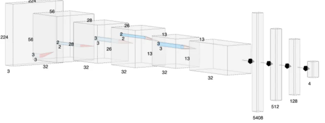
The proposed DNN consists of a feed forward fully connected network with 93 input units and 7 output units. The DNN hyperparameters have been tuned by running multiple tests in order to find the best configuration. In general, a good design choice is to start with a number of neurons in between the input and output units, for this reason we decided to use 80 neurons for each hidden layer. On the other hand, to determine the number of layers, we adopted a progressive

(36)

training approach which consists in starting with a single hidden layer and then progressively increase the number of layers until we reached a satisfying result in terms of accuracy and training time. After this procedure, we found that 6 hidden layers were sufficient to obtain a good model which was able to properly detect the user position inside the environment. The DNN architecture is showed in Figure 2.3.

..

.

..

.

..

.

..

.

..

.

I1 I2 I3 I93 H1 H80 H1 H80 O1 O7 Input layer Hidden layer 1 Hidden layer 6 Output layer

. . .

Figure 2.3: DNN architecture.

We selected the ReLU as activation function which resulted to be the best in terms of training time since it required a lower number of training iterations if compared with other activation functions like the Sigmoid (see Table 1.1). Then, we set the cross-entropy as cost function J as it is particularly suitable for classification problems, especially when used in combination with the softmax function. Softmax is a function that given an input vector z ∈ Rp_{, it produces as} output a vector ˜_{y ∈ R}p whose values add up to 1 and it is defined as follows:

˜ yj = Softmax(zj) = ezj Pp k=1ezk , j = 1, ..., p, (2.4)

(37)

given a fingerprint x. The cost function J is defined as:

J = −Xy · log(˜y), (2.5)

where the sum is extended to all the training samples. Cross-entropy represents a Maximum Likelihood Estimator (MLE) for the DNN hyperparameters vector θ. In other words, minimizing the cost function J corresponds to find the best set of parameters such that the parametric probability distribution learned by the model is the closest to the real data distribution (which is not known a priori). In particular, the cost function is minimized through the training process during which the weights of the DNN are iteratively adjusted to better fit the input data. To do this, we used adaptive momentum estimation (known as Adam optimizer) that maintains a different learning rate for each network weight and adapts it during the training process. Finally to prevent the problem of overfitting, we used a L2 regularization by adding a weighted penalization term:

penalization = λ · N X

L=1

W_L2, (2.6)

where N is the DNN number of layers, W_L2 are the squared weights of the L − th layer, and λ is the regularization rate (i.e., how much the penalization impacts the loss function). By adding this term to the loss function, we apply a penalization to the DNN weights thus reducing model complexity. DNN hyperparameters are summarized in Table 2.2.

Table 2.2: DNN hyperparameters. DNN configuration

# Hidden Layers 6

# Neurons per layer 80

Activation function ReLU

Learning rate 0.001

Regularization rate 0.01

(38)

The DNN implementation has been done using TensorFlow1 _{an open source}

framework developed by Google for the design of powerful machine and deep learning models [25].

Figure 2.4 shows how the cost function J decreases at each iteration (i.e., training epoch). The trend of the curve demonstrates that the DNN is able to correctly learn the relationship between a Wi-Fi fingerprint and a location inside the indoor environment. This is also confirmed by the 99.6% of accuracy reached by the network on the test set which represents a very good result in terms of generalization. 0 5000 10000 15000 20000 25000 Training epochs 0 1 2 3 4 5 6 7 J

Figure 2.4: The value of the cost function J with respect to the training epochs.

(39)

CHAPTER 2. SMART HOME int p r e d i c t ( f l o a t [] i n p u t ) { f l o a t [] r e s u l t = new f l o a t [ O U T P U T _ S I Z E ]; i n f e r e n c e I n t e r f a c e . f e e d ( I N P U T _ N O D E , input , I N P U T _ S I Z E ) ; i n f e r e n c e I n t e r f a c e . run ( O U T P U T _ N O D E S ) ; i n f e r e n c e I n t e r f a c e . f e t c h ( O U T P U T _ N O D E , r e s u l t ) ; r e t u r n a r g m a x ( r e s u l t ) ; }

Listing 2.1: Prediction Method.

2.1.3 Indoor localization system

To implement the system and test it in a real scenario, we realized two software sub-systems: i.) a Python server hosted in the Cloud to train the DNN; ii.) an Android application to create the Wi-Fi fingerprint dataset and to localize the user. For the dataset creation, we installed the app on several mobile devices to collect a large number of fingerprints by means of crowdsensing. The collected data is sent from the smartphone to the Cloud where the DNN is trained. Once the training phase is finished, the trained DNN model is sent to the Android clients in order to start the localization phase. In this sense, one of the main advantages of using TensorFlow consists in the possibility to store a trained model in a binary file that can be loaded into an Android environment. By doing this, the heavy computation for the DNN training is done on the Cloud, while the smartphone is only responsible for the inference task (i.e., the prediction) which runs locally without needing an Internet connection to localize the user.

Our trained model occupies just 148KB which is a very good result if we consider the complex DNN topology, and it is perfectly suitable to be loaded into the RAM of a mobile device. Thanks to the Application Programming Interfaces (APIs) provided by TensorFlow, the Android application is able to interact with the model by feeding it and retrieving the results.

With reference to the code showed in Listing 2.1 used for the prediction, the inferenceInterface object acts as a communication bridge between the app and the model, and exposes three methods:

(40)

• feed(): to feed the DNN with new input data; it takes as input three parameters, namely: the name of the input layer, the input data, and the input size.

• run(): to run the model and generate the output; it takes as parameter only the name of the output layer.

• fetch(): to fetch the results from the output layer passed as input; the results are stored in a float array containing (for this application) the prob-abilities of each class (i.e., the locations).

After calling the aforementioned methods, the prediction result is finally passed to the argmax function to return the most probable location where the user is located according to the input fingerprint.

From a structural point of view, we designed the Android app by splitting it into two parts: one for the learning and another one for the tracking of the user. With respect to the learning part, it is responsible to collect the labeled wireless fingerprints via multiple Wi-Fi scans. This is accomplished using the method getScanResults() provided by the WifiManager class of Android. During this phase, the user communicates the room where he is located by just tapping on the map showed on screen as depicted in Figure 2.5a.

When in “learn mode”, the user can decide to send one fingerprint through the button “SEND FINGERPRINT” or to send them continuously in background by tapping on “SEND (BKGD)”. Each time a scan finishes, all the data and the corresponding labels are stored on a json file and then sent to the server. The tracking part is responsible to localize the user inside the indoor environment and it is showed in Figure 2.5b. Like the previous case, also in “Track mode” the user can decide to be tracked only once or continuously by pressing the but-ton “TRACK ME” or “TRACK ME (BKGD)” respectively. During this phase, the DNN stored internally the application is fed with the MAC addresses and the corresponding RSSIs detected by the device to get a prediction of the most

(41)

(a) Learn Screen (b) Track Screen

Figure 2.5: Android application screenshots.

probable user location. Sometimes, it can happen that the app perceives new MAC address for which the DNN is not trained; since is not possible to change the neural network topology of a trained model, the application simply drops all those MAC addresses which are not contained in the features set F .

2.1.4 Localization results

We conducted a set of experiments to test how the DNN performs in a real indoor scenario to measure the accuracy and system response time while predicting the user location. In this experiment, a user is asked to follow a specific path and to notify the entrance in a room using a button displayed on the application. In

(42)

particular, this signal has been used as ground truth to be compared with the output of the trained DNN. At fixed time intervals T , a Wi-Fi scan is performed and passed to the DNN to predict the user location. For this experiment we set the time intervals T to 1 second. Such a choice resulted a good trade-off in terms of device energy consumption and prediction accuracy, considering a user moving at a normal walking speed (about 1.4 m/s).

Once we established the path to follow, we also fixed a residence time of 1 minute for each location (except for the M ainCorridor) during which the user is free to move inside the room without any type of constraint. By recalling Figure 2.1 and considering Room0 as starting point, the path traveled in this experiment is the following: Room0 → M ainCorridor → Room1 → M ainCorridor → Room2 → M ainCorridor → Room3 → M ainCorridor → Room4 → M ainCorridor → Room5 → M ainCorridor.

This in particular represents one of a large set of experiments we performed in the 7 − th floor of the engineering department. However, according to the empirical test we made, the path followed by the user did not affect the overall accuracy of the localization system which remained always in the same range.

Prediction Ground Truth 0 30 60 90 120 150 180 210 240 270 300 330 360 390 420 450 480 510 540 0 1 2 3 4 5 6 7 Prediction Ground Truth 0 1 2 3 4 5 6 7 Prediction Ground Truth 0 30 60 90 120 150 180 210 240 270 300 330 360 390 420 450 480 510 540 0 1 2 3 4 5 6 7 Prediction Ground Truth 0 30 60 90 120 150 180 210 240 270 300 330 360 390 420 450 480 510 540 0 1 2 3 4 5 6 7 Time (sec) a Location (Ground truth) Location (DNN prediction) a b b b b b a c c c

Room 0 Room1 Room 2 Room 3 Room 4 Room 5 Main Corridor

0 30 60 90 120 150 180 210 240 270 300 330 360 390 420 450 480 510

Figure 2.6: DNN prediction of the user location during a specific path taken as ground truth.

Figure 2.6 shows the comparison between the ground truth and the DNN prediction over time. The x-axis represents the time of the experiment (which lasted 520 seconds) while the colored bars represent the ground truth and the predicted user location. In general, the DNN was able to correctly detect the user position, however it generated some errors which we highlighted in Figure

(43)

2.6 with arrows labeled as a, b, and c representing three different error categories. The first error (category a) is generated by a localization prediction delay and indicated in the figure with a solid arrow. It is mainly caused by the fact that the ground truth trace is instantaneously updated by the user when he enters in a new location. On the other hand, the DNN trace depends on the time intervals T at which the scans are performed, on the time required to retrieve the results from the Wi-Fi scan, and on the time necessary to run the DNN and get the prediction. Even considering these aspects, the delay introduced by the system is acceptable and does degrade the quality of the localization.

The second error category (category b) is indicated by dashed arrows and rep-resents the DNN glitches during the inference phase. These errors, are caused by the DNN which makes a wrong prediction given a fingerprint as input. However, such a behavior is acceptable since the DNN is able to correctly detect the user for most part of the experiment.

Finally, the last category represented with dotted arrows labeled with c refers to a condition where the DNN is unable to localize the user when crossing the M ainCorridor. In particular when the user moves between two very near loca-tions e.g., Room1 and Room2 or Room3 and Room4 (as showed in Figure 2.1), the time necessary to move from a room to another is the order of a few seconds. The DNN is unable to catch such quick movements, thus resulting unable to de-tect the user position when he remains in the main corridor for a short period. Of course, this is a problem that happens only when the user moves between two near locations, in fact, by focusing on the last part of the experimental re-sults, we can observe that the DNN is able to correctly localize the user in the M ainCorridor when remaining for a longer time.

At the end of the experiment, the accuracy reached by the DNN on a “dy-namic” scenario was equal to 83.6% which is lower than the one obtained in the “static” test where we just fed the model with a test set. Nevertheless, the results obtained during this experiment are still good considering that the above

(44)

men-CHAPTER 2. SMART HOME

tioned errors become negligible in an application context where the user moves in an indoor environment remaining for long periods in the same location, and accessing services provided by smart objects inside of it.

(45)

Chapter 3 Smart Cities

In the recent period, smart cities have become an enabling technology for the development of infrastructures where applications can run. The Cloud paradigm plays a very important role for the realization of smart city scenarios, however, when working with applications which exhibit strict requirements in terms of latency and privacy, it becomes ineffective. In this chapter, we present two solu-tions that exploit AI and Edge computing technologies to improve applicasolu-tions performance in smart city contexts [26], [27].

3.1 Application relocation in Multi-access Edge

Computing

Multi-access Edge Computing (MEC) is an emerging paradigm which shifts data and computational resources near mobile users, with the goal of reducing ap-plications latency and improve resource utilization. Nowadays, smart services are becoming more resource demanding, requiring sometimes strict latencies that Cloud-based applications are unable to meet. In such a context, MEC standard-ized by the European Telecommunications Standards Institute (ETSI) can be considered a valid solution to address this problem [28]. MEC allows to move the Cloud capabilities at the edge of a mobile network, close to the users. Through

(46)

CHAPTER 3. SMART CITIES

this paradigm, we are able to strongly reduce the communication latency, while enabling the development of more effective services that can benefit their prox-imity to the user to extract context information (e.g., user position, real-time awareness of the radio-access network, etc.), by means of secure and controlled interfaces. Initially designed to be a part of the 4G architecture, MEC will play a key role for the upcoming 5G network where it will be implemented as part of the Network Functions Virtualisation architecture [29].

One of the main challenges in MEC consists in the application relocation. To exhibit a low latency, applications must follow the mobile users by relocating from a MEC server to another one [30]. Although the MEC exposes a set of functionalities that allow to relocate an application (or service) in a seamless way to the user, suitable policies have to be designed to decide if, when, and where an application should be relocated. A policy should also take into account several parameters e.g., the availability and the load of the destination server, the communication latency, the overhead caused by the relocation, etc., with the goal of optimizing the application Quality of Service (QoS). Moreover, if we consider that these policies should work not just for a single user, but on global scale and for a wide range of applications, it is more than evident how challenging is this problem.

3.1.1 MEC architecture

The core elements of the MEC architecture are the Mobile Edge (ME) Hosts [31]: nodes equipped with storage and computing capabilities placed very close to radio stations, thus allowing low latency and context-aware services to the User Equipments (UEs). Figure 3.1 (left) depicts the internal structure of a ME Host. It provides an environment to run ME Applications (MEApp) as Virtual Machines (VMs) instances on top of a Virtualisation Infrastructure (VI). The ME Platform (MEP) is responsible to instantiate and terminate the execution of MEApps and provides the access to useful services by means of APIs. In

Deep learning techniques for Intelligent Cyber Physical Systems: towards a new generation of smart and autonomous things

Universit`

a degli Studi di Messina

Department of Engineering

Doctoral Programme in Cyber Physical Systems

XXXIII Cycle

Deep Learning Techniques for Intelligent Cyber

Physical Systems: Towards a New Generation of

Smart and Autonomous Things

Student:

Fabrizio De Vita

Advisor:

Prof. Dario Bruneo

Co-Advisor:

Prof. Sajal K. Das

Contents

Abstract

Introduction

Chapter 1

Background

1.1

Intelligent Cyber Physical Systems

1.2

Machine learning

1.2.1

Artificial Neural Networks

Inputs

x

x

. . .

x

b

w

w

w

∑

f

y

Output

1.2.2

Deep learning

Chapter 2

Smart Home

2.1

Indoor user localization

2.1.1

Fingerprint dataset

2.1.2

Deep learning approach for indoor localization

..

.

..

.

..

.

..

.

..

.

. . .

2.1.3

Indoor localization system

2.1.4

Localization results

Chapter 3

Smart Cities

3.1

Application relocation in Multi-access Edge

Computing

3.1.1

MEC architecture

_b