Automatic discovery of drug mode of action and drug repositioning from gene expression data

PhD thesis in COMPUTER SCIENCE

Automatic Discovery of

Drug Mode of Action

and

Drug Repositioning

from Gene Expression Data

Candidate: Francesco Iorio

Supervisors:

Prof. Giancarlo Raiconi, Dr. Diego di Bernardo Coordinator:

Prof. Margherita Napoli

During my PhD training I have spent more than 3 years in the Systems, Synthetic and Computational Biology Laboratory (diB-LAB) led by Diego di Bernardo at the TeleThon Institute of Genetics and Medicine (TIGEM). I joined the group after my graduation in computer science, in a joint PhD program between the University of Salerno and the TIGEM.

When I arrived I felt like a stranger in a strange land: until that moment I used to deal mainly with numbers, codes and programming languages and from that moment I started to tackle molecular biology problems.

However I was really lucky because in that place I found nice people, with different backgrounds, talking to each other with ease, with humility and friendship. They taught me that true science is communication, knowledge sharing and creativity. They were the diB-LAB “first-generation” mem-bers: Mukesh Bansal, Giusy della Gatta, Alberto Ambesi-Impiombato, and Giulia Cuccato. Thanks!

I started my training program with three other PhD students. We grew together, learning from each other and we had really nice parties and a lot of fun: Thanks to Vincenzo Belcastro for helping me at different stages of my project, for giving me the opportunity to collaborate with him, and... for getting drunk together in different parts of the world; thanks to Velia Siciliano for kindly introducing me to the wonderful world of biotechnology experimental tools and for being one of the most “positive” people I have ever known; thanks to Lucia Marucci (mathematics, art, music, madness, genius and candor mixed together in an explosive recipe) for having been a real friend in some difficult moments.

our lab and my deskmate. Thanks also for giving to me the opportunity to work with him on NIRest and other algorithms.

During these years our lab was enriched by novel and really smart guys: Thanks to Filippo Menolascina for being the best lab-mate one could imag-ine and for listening to me patiently; Thanks to Gennaro Gambardella for being my personal Java trainer and “food-shopping-assistant”; Thanks to Mariaurelia Ricci and Alda Graziano for their kindness and friendship.

Thanks to Nicoletta Moretti (aka Alfia), Stefania Criscuolo, Immacolata Garzilli and Chiara Fracassi: we did not share the lab for a long time be-cause some of them joined our group in the last months of my permanence there and others were constantly involved in wet-lab experiments, but that time was sufficient to me to understand what nice people they are.

Thanks to Gennaro Oliva, of the ICAR institute, for his kind assistance and his (massive) competence, which were of great help to me during the implementation and management of the MANTRA web-tool.

Irene Cantone did incredible work, and I found IRMA to be one of the most exciting projects I encountered since I started to work in this field. However, I principally wish to thank this “mad” girl for her genuine and unruly friendship.

Thanks to Vincenza Maselli: truly one of the most kind and good-natured people I have ever met.

Thanks to the TIGEM bioinformatic-core for its support and kind help while I was dealing with statistical tests and microarray data. Rossella Rispoli, Gopuraja Dharmalingam, Annamaria Carissimo, and Margherita

inspired my work, for being the first person that patiently worked with me when I joined the TIGEM, and for her really fun jokes.

A really great special thanks to my friend Santosh Anand!

I wish to thank Graciana Diez-Roux for very critically reading and revising the manuscript of my most important paper.

A great thank you to Nicola Brunetti-Pierri that contributed ideas and the design of the research about Fasudil: a significant effort to my results. Thanks to Pratibha Mithbaokar and Rosa Ferriero, of the Brunetti-Pierri lab, doing the experiments that confirmed one of my nicest results.

Being a member of a TIGEM group has been one of the most stimulating experiences of my life. I wish to thank Maria Pia Cosma, who gave me the opportunity to collaborate with people in his lab in really great projects, and the other group leaders that involved me in their work: Alberto Auricchio, Giancarlo Parenti, and Alberto Luini. A great thank you to Seetharaman Parashuraman for the same reasons.

Working at TIGEM has been great and comfortable also because of the nice people working in the administration and human resources: Silvana Ruo-tolo, Federico Barone, Brunella Summaria, Barbara zimbardi, Mariolina Pepe et al. Thanks!

work, your kind assistance and all the nice chats and funny jokes.

What makes TIGEM a special place is each single person working there: thanks to Signor Agostino, Antonio and Dina. Your smiles were the best way to start each working day!

I want to thank my housemate Carmine Spampanato for having kindly put up with me for almost three long years.

Last but (obviously) not least a huge thank to Diego di Bernardo (my su-pervisor, at the TIGEM): literally the best mentor that anyone trying to do science could have!

He has an incredible ability in helping young scientists to discover (and to do) what they do best. He saw some little talent in me and cheered me up even in the most discouraging moments.

THANKS!

At the University of Salerno I have been working in the Neural and Robotic Network (NeuRoNe) Laboratory led by Prof. Roberto Tagliaferri and Prof. Giancarlo Raiconi.

I met these two Professors when I was an undergraduate and I wish to thank them for insightfully introducing me to the world of Machine Learn-ing, Data MinLearn-ing, Complex Systems and Neural Networks.

I wish to thank Loredana Murino (PhD student at the NeuRoNe lab) for her great work on the GO:Fuzzy-Enrichment analysis.

Thanks to Francesco “Ciccio” Napolitano: a real friend and one of the most intelligent and stimulating people I ever met.

Thanks to the people of the lab for their friendship and the time spent together: Andrea Raiconi, Carmine Cerrone, Donatella Granata, Ekaterina Nosova, Ivano Scoppetta (aka Vittorio Santoro), Francesco Carrabs and Ida Bifulco.

A huge thank you to Antonella Isacchi, Roberta Bosotti, and Emanuela Scacheri of the Nerviano Medical Science conceiving the blind test of my method, for producing novel Microarray-Data for me and performing the experiments validating some of my most original and interesting results. Additionally, thanks to them for their great contribution to my paper, for their help in interpreting MANTRA results, their great expertise in on-cology and the extremely stimulating chats we had via Skype, Phone and Email.

A great team: it has been really a pleasure to work with them. THANKS Nerviane!

A special thanks to Dr. Julio Saez-Rodriguez for hosting me in his labo-ratory at the European Bionformatics Institute in the last months of my PhD, for giving me the opportunity of joining a great group and the chance

Thanks to my new lab-mates (both the temporary and the permanent ones): Beatriz Penalver, Ioannis Melas, Camille Terfve, Jordi Serra i Musach, Aidan MacNamara, Jerry Wu and David Henriques.

Thanks to Gabriella Rustici for her kind help when myself and my fam-ily were searching for accommodation in Cambridge and for her friendship.

Now it is the turn of the most important people in my life...

First of all, I wish to thank my parents, who always supported me in every possible way. I believe that they should be cited as co-authors of this and all the other successes in my life. Mum and Dad: I love you.

Secondly, I want to thanks my in-laws: they were literally my second par-ents in these last few years and helped the little new family that myself and my wife were composing with infinite love and patience. Nonna Brenda and Nonno Pasquale: a huge THANK YOU and a hug!

A huge hug and a thank you to my “brothers and sisters”:

Ylenia, Giuseppe (the greatest mathematician I have ever known) and Raf-faella, Davide and Annarita, for their love and all the funny moments to-gether.

happiness. To say “thank you” would be improper, as is improper (and impossible) to list all the reasons why I should do it. Annalisa, I love you and I am so happy you are my wife.

Finally, to you: I hope that your eyes will always be full of this curiosity and vivacity, and that you will look at me always as you do now; I hope to deserve your love for ever and that your smiles will be always so real and happy.

The identification of the molecular pathway that is targeted by a compound, combined with the dissection of the following reactions in the cellular envi-ronment, i.e. the drug mode of action, is a key challenge in biomedicine. Elucidation of drug mode of action has been attempted, in the past, with different approaches. Methods based only on transcriptional responses are those requiring the least amount of information and can be quickly applied to new compounds. On the other hand, they have met with limited success and, at the present, a general, robust and efficient gene-expression based method to study drugs in mammalian systems is still missing.

We developed an efficient analysis framework to investigate the mode of action of drugs by using gene expression data only. Particularly, by using a large compendium of gene expression profiles following treatments with more than 1,000 compounds on different human cell lines, we were able to extract a synthetic consensual transcriptional response for each of the tested compounds. This was obtained by developing an original rank merg-ing procedure. Then, we designed a novel similarity measure among the transcriptional responses to each drug, endingending up with a “drug sim-ilarity network”, where each drug is a node and edges represent significant similarities between drugs.

By means of a novel hierarchical clustering algorithm, we then provided this network with a modular topology, contanining groups of highly inter-connected nodes (i.e. network communities) whose exemplars form second-level modules (i.e. network rich-clubs), and so on. We showed that these topological modules are enriched for a given mode of action and that the hierarchy of the resulting final network reflects the different levels of simi-larities among the composing compound mode of actions.

potential therapeutic applications can be assigned to safe and approved drugs, that are already present in the network, by studying their neighbor-hood (i.e. drug repositioning), hence in a very cheap, easy and fast way, without the need of additional experiments.

By using this approach, we were able to correctly classify novel anti-cancer compounds; to predict and experimentally validate an unexpected similar-ity in the mode of action of CDK2 inhibitors and TopoIsomerase inhibitors and to predict that Fasudil, a known and FDA-approved cardiotonic agent, could be repositioned as novel enhancer of cellular autophagy.

Due to the extremely safe profile of this drug and its potential ability to traverse the blood-brain barrier, this could have strong implications in the treatment of several human neurodegenerative disorders, such as Hunting-ton and Parkinson diseases.

List of Figures xv

List of Tables xix

List of Algorithms xxi

1 Introduction 1

1.1 Outline . . . 5

2 Background 9 2.1 Introduction . . . 9

2.2 Molecular biology: basic principles and techniques . . . 10

2.2.1 Overview of the Cell . . . 10

2.2.2 DNA structure and function . . . 12

2.2.3 Gene Expression and Regulation . . . 17

2.2.4 How to measure gene expression level . . . 18

2.2.5 Protein detection and localization assays . . . 25

2.3 Network Theory: basic principles . . . 27

2.3.1 Networks as alternative to euclidean embeddings . . . 30

2.4 Computational Drug Discovery . . . 32

2.5 Network analysis improves understanding of drug use and effects . . . . 35

3 Gene Expression Based Methods and Systems Biology 37 3.1 Introduction . . . 37

3.1.1 Inference of Gene Regulatory Network . . . 37

3.1.2 The Network Inference by multiple Regression (NIR) algorithms 39 3.1.3 The DREAM initiative . . . 42

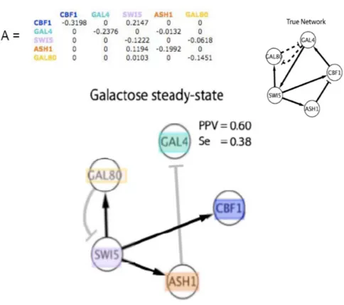
3.1.4 The IRMA project: In-vivo Reverse-engineering and Modelling

Assessment . . . 42

3.2 Analysis of Phenotypic Changes . . . 44

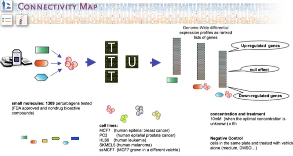
3.2.1 The Connectivity Map dataset . . . 47

3.3 Gene Signature Based Methods . . . 48

3.3.1 Gene Set Enrichment Analysis . . . 49

3.3.2 The Connectivity Map query system . . . 49

3.4 A first pilot study . . . 50

4 A novel computational framework for Drug Discovery 55 4.1 Introduction . . . 55

4.2 Synthetic Consensual Responses to Drugs . . . 56

4.2.1 How to merge ranked lists of objects . . . 59

4.2.2 Adaptive weighting of individual cell responses . . . 60

4.2.3 Spearman’s Footrule . . . 60

4.2.4 The Kruskal-Borda (KRUBOR) algorithm . . . 61

4.3 Drug distance Measure . . . 63

4.3.1 Drug Optimal Signature . . . 63

4.3.2 Computation of the distance between two drugs . . . 63

4.4 Distance assessment . . . 64

4.4.1 Gold-Standard Definition . . . 64

4.4.2 Assessment Methodology . . . 71

4.4.3 Results . . . 72

4.5 From pair-wise similarities to Drug-Network . . . 73

4.5.1 Network Evolution . . . 73

4.5.2 Statistical significance of the Drug Distance . . . 76

4.5.3 The final Drug Network . . . 77

4.5.4 Network Robustness . . . 77

4.6 Community Identification and Topological analysis . . . 79

4.6.1 Girvan-Newman Algorithm for finding communities in complex networks . . . 80

4.6.3 Building a modular network by recursive affinity propagation

clustering . . . 89

4.7 Network Assessment . . . 95

4.7.1 Statistical Testing . . . 97

4.7.2 Community enrichments . . . 98

4.7.3 Mode of Action enrichments . . . 98

4.7.4 Network hierarchy reflects different degrees of similarity . . . 99

4.7.5 Influence of Chemical Commonalities on drug distance and net-work topology . . . 101

4.7.6 Gene Ontology Fuzzy-Enrichment analysis of the communities . 104 4.8 Goals of a drug network with modular and characterized topology . . . 112

5 MANTRA: Mode of Action by NeTwork Analysis 115 5.1 Introduction . . . 115

5.2 Drug-to-Community Distance . . . 116

5.3 Classification Algorithm . . . 116

5.4 MANTRA web-tool . . . 119

6 Experimental validation of MANTRA predictions using known and novel chemotherapeutic agents 123 6.1 Introduction . . . 123

6.2 A “blind” classification test . . . 124

6.2.1 Experimental Setting and protocols . . . 124

6.2.2 Heat Shock Protein 90 (Hsp90) Inhibitors . . . 126

6.2.3 Cyclin-Dependent kinase (CDK) 2 Inhibitors . . . 128

6.3 Classification results . . . 130

6.3.1 Topoisomerase Inhibitors . . . 133

6.4 MANTRA highlights previously unreported similarities . . . 135

6.5 Classification Performance assessment and comparison with other tools . 137 6.6 Rank Merging Impact on the performances . . . 144

7 MANTRA predicts candidates for Drug Repositioning 149

7.1 Introduction . . . 149

7.2 Overview of the mechanism of cellular autophagy . . . 149

7.3 Drug repositioning proposals through established-drug neighborhood anal-ysis . . . 152

7.4 MANTRA predicts that Fasudil promotes cellular autophagy . . . 156

7.5 Experimental validation . . . 157

7.6 Hypotheses and consequences . . . 158

7.7 Discussion . . . 160

8 Future directions and Discussion 163 8.1 Introduction . . . 163

8.2 Cross platform/species compatibility . . . 163

8.3 Classification of diseases . . . 166

8.4 Conclusions . . . 170

References 173 A Abbreviations 179 B Community enrichments 181 B.1 Literature based evidences . . . 181

B.2 Anatomical Therapeutic Chemical (ATC)-Codes . . . 194

B.3 Molecular direct targets . . . 206

C Mode of Action enrichments 209 C.1 ATC codes . . . 209

C.2 Molecular direct targets . . . 215

D Electrotopological States (ESF) similarity and communities 219

E cMap online tool results 221

F Neighborhood of the tested compounds in the drug network 227

1.1 Discovery of drug mode of action . . . 1

1.2 Reactions to drug-substrate interaction . . . 2

1.3 Project: Leading ideas and problems . . . 4

2.1 The cell . . . 11

2.2 DNA . . . 13

2.3 The central dogma of molecular biology . . . 16

2.4 Protein synthesis . . . 16

2.5 A view of gene regulation . . . 18

2.6 Polymerase chain reaction . . . 19

2.7 Polymerase chain reaction . . . 20

2.8 Polymerase chain reaction . . . 20

2.9 Realtime PCR outcomes . . . 21

2.10 cDNA Microarray technology . . . 23

2.11 Affymetrix GeneChip Scheme . . . 24

2.12 Immunoblotting . . . 26

2.13 Indirect immunofluorescence . . . 28

2.14 Examples of networks . . . 29

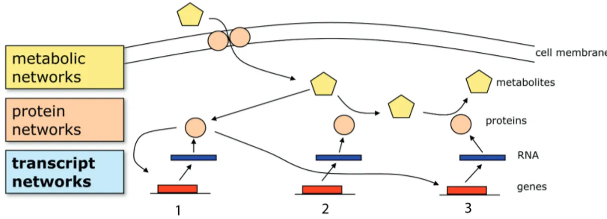
3.1 Biological network layers . . . 38

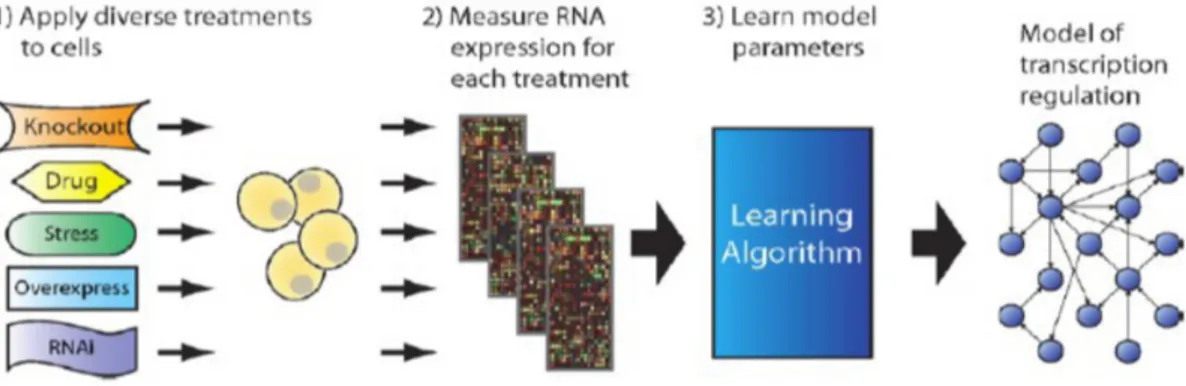
3.2 Computational pipeline . . . 39

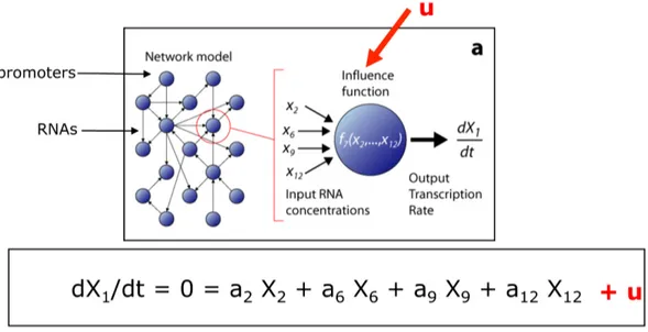
3.3 The NIR assumption . . . 40

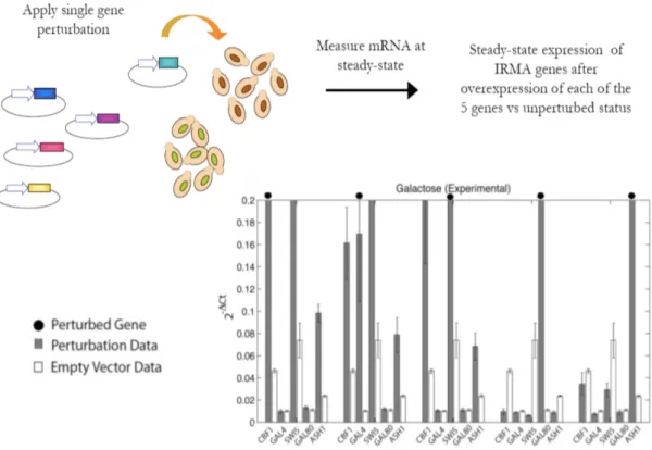
3.4 IRMA . . . 43

3.6 Inferring In-vivo Reverse-engineering and Modelling Assessment (IRMA)

with NIR . . . 46

3.7 The Connectivity Map . . . 48

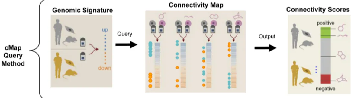
3.8 cMap query method . . . 50

3.9 Profile-wise GSEA . . . 52

3.10 Distance performances . . . 52

3.11 Distance performances . . . 53

4.1 Methodology overview . . . 57

4.2 Synthetic consensual response to the drug . . . 59

4.3 Cellular response variability three . . . 62

4.4 Average Enrichment-Score (AES) distance empirical pdf . . . 65

4.5 Maximum Enrichment-Score (MES) distance empirical pdf . . . 65

4.6 ATC code example . . . 67

4.7 Drug distance performances . . . 72

4.8 Network evolution . . . 75

4.9 Final network . . . 78

4.10 Network statistics . . . 79

4.11 Girvan-Newman network communities . . . 84

4.12 Affinity propagation algorithm . . . 88

4.13 Drug communities . . . 91

4.14 The Drug Network . . . 94

4.15 Post-processed network statistics . . . 95

4.16 NeTwork by Recursive Affinity Propagation (N-TRAP) communities contain similar drugs . . . 96

4.17 Community enrichments . . . 99

4.18 Mode of Actions (MoAs) enrichments . . . 100

4.19 Hierarchy of similarities and topology . . . 101

4.20 Correlation with chemical similarity . . . 103

4.21 Influence of chemical similarity on drug distance . . . 104

4.22 Modularity and performances . . . 114

5.1 MANTRA . . . 120

6.1 Classification results . . . 134

6.2 Inhibition of CDKs by doxorubicin and SN-38 . . . 135

6.3 Down-stream effects of CDK2 and Topoisomerase (Topo) inhibitors . . . 136

6.4 Effects on p21 and CDK2 substrates . . . 137

6.5 Effects on RNA pol II . . . 138

6.6 Individual Gene Expression Profiles (GEPs) distance assessment . . . . 144

7.1 Cellular Autophagy . . . 150

7.2 Autophagic pathways . . . 151

7.3 2-deoxy-d-glucose closest neighbors . . . 153

7.4 Effects of fasudil on autophagy (1) . . . 158

7.5 Effects of fasudil on autophagy (2) . . . 159

7.6 Effects of fasudil on autophagy (3) . . . 160

8.1 Cross-platform conserved genes . . . 165

8.2 Pilot study results on mouse data . . . 167

4.1 ATC codes, 1st Level . . . 68

4.2 ATC codes, 2nd Level of the B tree . . . 68

4.3 ATC codes, 2nd Level of the L tree . . . 68

4.4 ATC codes, 3rd Level of the C tree in C01 sub-tree . . . 69

4.5 ATC codes, 3rd Level of the L tree in L02 sub-tree . . . 69

4.6 ATC codes, 4th Level in the L02B sub-tree . . . 70

4.7 ATC codes, 4th Level in the L02B sub-tree . . . 70

4.8 Communities identified with the modified Girvan-Newman algorithm (a) 85 4.9 Communities identified with the modified Girvan-Newman algorithm (b) 86 4.10 GO:Fuzzy enrichment analysis - Community 28 . . . 109

4.11 GO:Fuzzy enrichment analysis - Community 14 . . . 110

4.12 GO:Fuzzy enrichment analysis - Community 63 . . . 111

4.13 GO:Fuzzy enrichment analysis - Community 28 . . . 112

6.1 CDK inhibitors selectivity . . . 130

6.2 Tested compounds neighbors . . . 131

6.3 Tested compounds neighboring communities . . . 132

6.4 cMap tool analyzed compounds . . . 139

6.5 Distance performances . . . 140

6.6 Classification performances . . . 141

6.7 NMS-doxorubicin case . . . 143

6.8 Rank merging and performances . . . 145

7.1 2-deoxy-D-glucose (2DOG) neighborhood . . . 154

7.3 2DOG rich-club . . . 155 8.1 Classification results on mouse data . . . 167

1 KRUBOR merging method . . . 61 2 Modified Girvan-Newman . . . 82 3 N-TRAP . . . 92 4 GO:Fuzzy-Enrichment-Analysis . . . 108 5 Drug-Classification . . . 117

Introduction

A bottleneck in drug discovery is the identification of the molecular targets of a com-pound and of its off-target effects (Figure 1.1).

Figure 1.1: Discovery of drug mode of action

-The recognition of a set of interacting genes, proteins and metabolites (i.e. a bi-ological pathway) whose activity is modulated by the drug treatment, combined with the dissection of the resulting reactions in the cellular environment (Figure 1.2), is nowadays a key challenge in biomedicine.

Addressing these problems means to investigate drug Mode of Action (MoA). On the other hand, the detection of the complex regulatory relationships occurring

Figure 1.2: Reactions to drugsubstrate interaction

-among genes (i.e. gene regulatory network) is of major importance in order to under-stand the working mechanisms of the cell in patho-physiological conditions and it also allows the discovery of novel drug targets.

Thanks to the development of new experimental methods and to the constant decrease of the data-storage costs, current technology allows the analysis of massive quantities of data. One of the scientific fields that are taking great advantages of this capabilities is molecular biology in which a key role is played by DNA-microarray technology, in the context of functional genomics.

Each single cell contains a copy of the entire genome of the organism to which it be-longs.

The genome is composed by DNA molecules and it contains the set of informations needed for the transmission of the hereditary factors and the protein synthesis. Once a gene is “activated” a corresponding molecular intermediate, the messenger RNA (mRNA), is generated through a process called “transcription” and released in the cy-toplasm (the thick liquid residing among the nucleus, the cellular membrane and the organelles). Here, the mRNA is translated into proteins through the assembly of amino acids by a ribosomes.

The amount of mRNA equivalent to the DNA sequence of a given gene, in a give in-stant, quantifies the “level of expression” of that gene.

file (GEP)). By using DNA-microrrays it is possible to monitor the expression of all the genes in the cells of a given tissue in pathological conditions or to measure how cells respond to a pharmacological treatment at a transcriptional level.

Even if elucidation of drug MoAs has been attempted, in the past, with different ap-proaches, the drug discovery pipeline typically has been guided by knowledge of the biological mechanisms underlying the disease to treat. Based on this knowledge, “drug-gable” molecular targets have been hypothesized and libraries of chemical structures have been systematically analyzed in order to find drug candidates on the basis of their chemical “affinity” with the desired target.

More recently, alternative approaches such as high-throughput screening of drug li-braries have been developed to allow identification of molecules acting on specific cel-lular targets experimentally. However, they are generally based on assays or binding studies that focus narrowly on the molecular target, not taking into account the com-plexity of the cell response.

Strategies based on the analysis of drug-induced changes in gene expression profiles have the potential to elucidate the cellular response to specific drugs. Moreover, meth-ods based only on transcriptional responses are those requiring the least amount of experiments and can be quickly applied to new compounds. On the other hand, they have met with limited success and, at the present, a general, robust and efficient gene-expression based method to study drugs in mammalian systems is still missing. Other important problems are linked to the concept of “drug repositioning”: the large number of drug candidate failures has been enormously costly for the pharmaceuti-cal industry, but has also created the opportunity of re-purposing these molecules for therapeutic applications into new disease areas. Companies which can systematically “reposition” unsuccessful drug candidates could create significant value by reinforcing their pipeline (the set of drugs under development or in testing) and meeting the needs of innovative medicines.

In this PhD thesis we present the methodology and the results of our research, which has been focused on the development of a novel and efficient analysis framework to in-vestigate the MoA of new drugs by using gene expression data only and for suggesting novel therapeutic uses of well-known and already approved drugs.

Our leading assumption was a simple but strong postulate: if two drugs elicit similar effects on the transcriptional activity of the cell then they could share a MoA (and pos-sibly a therapeutic application) even if they act on distinct intracellular direct targets (point 1 in Figure 1.3).

Figure 1.3: Project: Leading ideas and problems

-As a consequence, similarities in the transcriptional responses to drugs could be ex-ploited allowing drug classification and repositioning (i.e. re-purposing for novel uses) (point 2 in Figure 1.3). The first problem we had to tackle was due to a phenomenon known for microarray studies: cells grown at the same time and in the same experimen-tal setting tend to respond similarly at a transcriptional level even if they are differently stimulated. In other word similarity of gene expression profiles can be recorded for un-related stimuli in the same experimental setting (also called batch effect)(81). On the other hand, cells in different pathological conditions obey to the rules of the transcrip-tional program in the corresponding disease phenotype (the condition characteristics) hence they tend to respond differently to the same drug treatment. Consequently, poor results can be achieved with classic micro-array analysis approach, which tends to

dis-criminate gene expression profiles on the basis of the experimental settings (kind of cells, observation time, microarray platform) in which they have been produced rather than on the basis of the stimuli they are responding to (for example a drug treatment) (point 3 in Figure 1.3).

We addressed this problem by using a large compendium of gene expression data fol-lowing treatments with more than 1,000 compounds on different human cell lines, being able to compute a synthetic consensual transcriptional response for each of the tested compounds. This response is a proxy of a “phenotype independent” transcriptional response and we considered it a sufficiently general summary of the drug MoA (point 4 in Figure 1.3). This was obtained by using a novel and original data merging procedure. In order to pair-wise compare the drugs in our reference dataset (point 5 in Figure 1.3) we conceived a novel similarity measure among these responses, which was based on a non-parametric statistic, ending up to a “drug similarity network” (point 6 in Figure 1.3).

Finally we used this network as a classification template and as a predictor of drug can-didates for drug repositioning, a task which has been growing in importance in the last few years as an increasing number of drug development and pharmaceutical companies see their drug pipelines drying up. To assess our results, novel experimental data were produced on purpose in order to validate computational predictions.

1.1

Outline

This thesis in computer science describes a computational approach to a practical prob-lem of drug discovery, which has been tackled based on principles of molecular biology and making use of available biomedical data.

Moreover, a number of experiments has been conducted with different experimental tools in order to produce de-novo data and to verify computational results. Some bi-ological concepts and principles together with the background informations needed to understand the experiment outcomes are provided in Chapter 2.

In the same chapter we covered some concepts from complex network theory and tra-ditional drug discovery. In Chapter 3 we briefly discuss gene expression and systems biology approaches to drug discovery.

we present Mode of Action by Network Analysis (MANTRA), the online implementa-tion of our method, and we describe the drug classificaimplementa-tion algorithm.

In Chapter 6 we present the results that were obtained while testing our method in classifying novel drugs and their experimental validation.

Chapter 7 contains the description of a drug repositioning proposal predicted by our method. Future directions and a final discussion are presented in Chapter 8.

Part of the work described in this thesis has been published in: • Iorio F, Isacchi A, di Bernardo D, Brunetti-Pierri N.

Identification of small molecules enhancing autophagic function from drug net-work analysis.

Autophagy. 2010 Nov 16; 6(8): 1204-5.

• Iorio F, Bosotti R, Scacheri E, Belcastro V, Mithbaokar P, Ferriero R, Murino L, Tagliaferri R, Brunetti-Pierri N, Isacchi A, di Bernardo D.

Discovery of drug mode of action and drug repositioning from transcriptional responses.

Proc Natl Acad Sci U S A. 2010 Aug 17; 107(33): 14621-6. • Iorio F, Murino L, di Bernardo D, Raiconi G, Tagliaferri R.

Gene ontology fuzzy-enrichment analysis to investigate drug mode-of-action Neural Networks (IJCNN), The 2010 International Joint Conference on. 2010 July: 1-7.

• Cantone I, Marucci L, Iorio F, Ricci MA, Belcastro V, Bansal M, Santini S, di Bernardo M, di Bernardo D, Cosma MP.

A yeast synthetic network for in vivo assessment of reverse-engineering and mod-eling approaches.

Cell. 2009 Apr 3; 137(1): 172-81. • Lauria M, Iorio F, di Bernardo D.

NIRest: a tool for gene network and mode of action inference. Ann N Y Acad Sci. 2009 Mar; 1158: 257-64.

• Iorio F, Tagliaferri R, di Bernardo D.

Identifying network of drug mode of action by gene expression profiling. J Comput Biol. 2009 Feb; 16(2): 241-51.

• Iorio F, Tagliaferri R, di Bernardo D.

Building Maps of Drugs Mode-of-Action from Gene Expression Data

Computational Intelligence Methods for Bioinformatics and Biostatistics. LNCS. 2009, Volume 5488/2009, 56-65.

Supplementary data sheets referred in the text are contained in the Supplementary Data Disc (SDD) attached to this thesis.

Background

2.1

Introduction

This chapter contains basic informations, needed to fully understand the biology under-lying the main presented results the experimental data that we analyzed and produced “de-novo”, and a short description of the experimental platforms that we used to verify our results (Section 2.2).

In Section 2.3 some definitions and methods of network theory that we used while de-signing our computational approach are listed.

In the final section computational drug discovery is briefly discussed and existing ap-plications of network analysis in this field are introduced.

The content of this chapter (figures and some portions of text) are from the following web resources: www.nigms.nih.gov, www.ebi.ac.uk, www.wordiq.com, www.bio.davidson.edu, www.molegro.com.

2.2

Molecular biology: basic principles and techniques

A cell is the simplest and most elementary functional basic unit of life and it can be considered as the building block of all living beings. Some organisms, such as most bacteria, consist of a single cell (unicellular organisms) while others, such as humans, are composed by about 100 trillion of cells.

In an “eukaryotic” cell (see Figure 2.1) the nucleus is a membrane enclosed organelle that can occupy up to 10 percent of the cellular space. It contains the equivalent of the cell’s “program”, its genetic material, the Deoxyribonucleic acid (DNA). DNA contains the instructions used in the development and functioning of all known living organisms with the exception of some viruses. The main role of DNA molecules is the long-term storage of information. DNA is often compared to a set of blueprints, like a recipe or a code, since it contains the instructions needed to construct other components of cells, such as proteins and Ribonucleic acid (RNA) molecules. The DNA segments that carry this genetic information are called genes, but other DNA sequences have struc-tural purposes, or are involved in regulating the use of this genetic information. The nucleus is surrounded by two pliable membranes, together known as the nuclear en-velope. Normally, the nuclear envelope is pockmarked with octagonal pits and hemmed in by raised sides. These nuclear pores allow chemical messages to exit and enter the nucleus.

Between the cell membrane (a selectively-permeable phospholipidic layer) and the nu-clear envelope resides a thick and nu-clear liquid called the cytoplasm. The cell’s outer membrane is made up of a mix of proteins and lipids (fats). Lipids give membranes their flexibility. Proteins transmit chemical messages into the cell, and they also mon-itor and maintain the cell’s chemical climate.

On the outside of cell membranes, attached to some of the proteins and lipids, are chains of sugar molecules that help each cell type do its job.

Close to the nucleus resides a groups of interconnected sacs snuggling close by. This network of sacs, the Endoplasmatic Reticulum (ER), often makes up more than 10 percent of a cell’s total volume.

that we will describe later), ribosomes have a critical job: assembling all the cell’s pro-teins. To make a protein, ribosomes weld together chemical building blocks one by one (as explained in the following sections).

Another important component of the cellular endomembrane system (the set of differ-ent membranes that are suspended in the cytoplasm) is the Golgi apparatus. Composed of stacks of membrane-bound structures known as cisternae, the Golgi apparatus pro-cesses and packages macromolecules, such as proteins and lipids, after their synthesis and before they make their way to their destination; it is particularly important in the processing of proteins for secretion.

The waste disposal system of the cell is composed by the lysosomal machinery. Lyso-somes are cellular organelles which contain acid hydrolase enzymes to break up waste materials and cellular debris.

Figure 2.1: The cell - [Image from: http://www.ebi.ac.uk]

The subtle movements of the cell as well as the many chemical reactions that take place inside organelles require vast amounts of cellular energy. The main energy source of the cell is a small molecule called Adenosine-5’-triphosphate (ATP). ATP is often referred as the “molecular unit of currency” of intracellular energy transfer because it transports chemical energy within cells for metabolism. It is produced by membrane-enclosed organelles called mitochondria. ATP is used by enzymes and structural pro-teins in many cellular processes, including biosynthetic reactions, motility, and cell division. Among these processes one of the most important is phosphorilation.

molecule (such as ATP) to a protein (in this case, a substrate). Phosphorylation is conducted by specific enzymes called phosphotransferases or kinases, it activates or deactivates many protein enzymes, causing or preventing the mechanisms of diseases such as cancer and diabetes. Protein phosphorylation in particular plays a significant role in a wide range of cellular processes and usually it results in a functional change of the target protein by changing enzyme activity, cellular location, or association with other proteins.

The series of events that takes place in a cell leading to its division and duplication (replication) is called the cell cycle, or cell-division cycle. Cell cycle is tightly regulated by the activity of a group of protein kinases, i.e. Cyclin-Dependent kinases (CDKs). A CDK is activated by association with a cyclin, forming a cyclin-dependent kinase complex. Cyclins are proteins whose concentrations varies in a cyclical fashion during the cell cycle. The oscillations of the cyclins, namely fluctuations in cyclin gene expres-sion and destruction by proteolysis, induce oscillations in CDK activity to drive the cell cycle.

A normal component of the development and health of multicellular organisms is cel-lular apoptosis, or programmed cell death. Cells die in response to a variety of stimuli and during apoptosis they do so in a controlled, regulated fashion. This makes apop-tosis distinct from another form of cell death called necrosis in which uncontrolled cell death leads to lysis of cells, inflammatory responses and, potentially, to serious health problems. Apoptosis, by contrast, is a process in which cells play an active role in their own death (which is why apoptosis is often referred to as cell suicide).

2.2.2 DNA structure and function

DNA is the main information carrier molecule in a cell. A single stranded DNA

molecule, also called a polynucleotide, is a chain of small molecules, called nucleotides (see Figure 2.2). There are four different nucleotides grouped into two types, purines: adenine and guanine and pyrimidines: cytosine and thymine. They are usually referred to as bases and denoted by their initial letters, A, C, G and T. Different nucleotides can be linked together in any order to form a polynucleotide. The end of the polynucleotides are marked either 5’ and 3’ . By convention DNA is usually written with 5’ left and 3’ right, with the coding strand at top. Two such strands are termed complementary, if one can be obtained from the other by mutually exchanging A with T and C with G,

and changing the direction of the molecule to the opposite. Although such interactions are individually weak, when two longer complementary polynucleotide chains meet, they tend to stick together.

Two complementary polynucleotide chains form a stable structure, which resembles a helix and is known as a the DNA double helix. About 10 base pairs (bp) in this struc-ture takes a full turn, which is about 3.4 nm long. Complementarity of two strands in the DNA is exploited for copying (multiplying) DNA molecules in a process known as the DNA replication, in which one double stranded DNA is replicated into two iden-tical ones. (The DNA double helix unwinds and forks during the process, and a new complimentary strand is synthesized by specific molecular machinery on each branch of the fork. After the process is finished there are two DNA molecules identical to the original one.) In a cell this happens during the cell division and a copy identical to the original goes to each of the new cells.

Figure 2.2: DNA - [Image from: http://www.scq.ubc.ca]

During replication an enzyme called Topoisomerase (Topo) prevents DNA tangling and damaging. As a replication fork moves along double-stranded DNA, it creates what

has been called the “winding problem”. Every 10 bp replicated at the fork corresponds to one complete turn about the axis of the parental double helix. Therefore, for a replication fork to move, the entire chromosome ahead of the fork would normally have to rotate rapidly. This would require large amounts of energy for long chromosomes, and an alternative strategy is used instead: a swivel is formed in the DNA helix by DNA Topo.

DNA winds around proteins called histones. These proteins play an important role in gene regulation in eukaryotic cells and they are are highly water soluble. The six histone classes are H1, H2A, H2B, H3, H4, and Archaeal. All but the H1 and Archaeal classes create nucleosome core particles by wrapping DNA around their protein spools; the H1 then binds nucleosomes and entry and exit sites of the DNA. Histones and DNA assembled in this way are called chromatin. Packed in this way DNA are 50,000 times shorter than unpacked ones. Histones also perform a function in gene regulation; their “methylation” (modification of certain amino acids by the addition of one, two, or three methyl groups) causes tighter bindings to down-regulate or even inhibit gene transcription, while “acetylation” (addition of acetyl groups) loosens bindings to help encourage transcription and translation.

Histone proteins are packaged into structures called chromosomes. Chromosomes are not visible in the cells nucleus, not even under a microscope, when the cell is not di-viding. However, the DNA that makes up chromosomes becomes more tightly packed during cell division and is then visible under a microscope. Most of what researchers know about chromosomes was learned by observing chromosomes during cell division. Each chromosome has a constriction point called the centromere, which divides the chromosome into two sections, or “arms”. The short arm of the chromosome is labeled the “p arm”. The long arm of the chromosome is labeled the “q arm”. The location of the centromere on each chromosome gives the chromosome its characteristic shape, and can be used to help describe the location of specific genes.

Together with DNA and proteins, RNA is one of the major macromolecules that are essential for all known forms of life. The sequence of nucleotides composing a molecule of RNA allows it to encode genetic information. For example, some viruses use RNA instead of DNA as their genetic material, and all organisms use messenger messenger

RNA (mRNA) to carry the genetic information that directs the synthesis of proteins. This process can be divided into two parts (as summarized in Figure 2.3):

• T ranscription: Before the synthesis of a protein begins, the corresponding RNA molecule is produced by RNA transcription. One strand of the DNA double helix is used as a template by the RNA polymerase to synthesize an mRNA. This mRNA migrates from the nucleus to the cytoplasm. During this step, mRNA goes through different types of maturation including one called splicing when the non-coding sequences are eliminated. The coding mRNA sequence can be described as a unit of three nucleotides called a codon;

• T ranslation: The ribosome binds to the mRNA at the start codon (AUG) that is recognized only by the initiator Transfer RNA (tRNA) (a small RNA molecule that transfers a specific active amino acid to the ribosome). The ribosome pro-ceeds to the elongation phase of protein synthesis. During this stage, complexes, composed of an amino acid linked to tRNA, sequentially bind to the appropriate codon in mRNA by forming complementary base pairs with the tRNA anticodon. The ribosome moves from codon to codon along the mRNA. Amino acids are added one by one, translated into polypeptidic sequences dictated by DNA and represented by mRNA (Figure 2.4). At the end, a release factor binds to the stop codon, terminating translation and releasing the complete polypeptide from the ribosome.

The rule that deals with the detailed residue-by-residue transfer of sequential infor-mation establishing that inforinfor-mation cannot be transferred back from protein to either protein or nucleic acid is known as the “central dogma of molecular biology”. In other words, once information gets into protein, it can’t flow back to nucleic acid.

Like shoelaces, the polypeptidic sequences released by the ribosomes loop about each other in a variety of ways (i.e., they fold). But, as with a shoelace, only one of these many ways allows the protein to function properly. Yet lack of function is not always the worst scenario. For just as a hopelessly knotted shoelace could be worse than one that wont stay tied, too much of a misfolded protein could be worse than too little of a normally folded one. This is because a misfolded protein can actually poison the cells around it.

Figure 2.3: The central dogma of molecular biology - [Image from: http://www.scq.ubc.ca]

2.2.3 Gene Expression and Regulation

Living cells are the product of gene expression programs involving “regulated” tran-scription of thousands of genes. The central dogma, briefly introduced in the previous section, defines a paradigm in molecular biology: genes are perpetuated as sequences of nucleic acid and translated in functional units, i.e. the proteins. In these process mRNA provides a molecular intermediate that carries the copy of a DNA sequence that represents a protein. It is a single-stranded RNA identical in sequence with one of the strands of the duplex DNA. In protein-coding genes, translation will convert the nucleotide sequence of mRNA into the sequence of amino acids comprising a protein. This transformation of information (from gene to gene product) called gene expression. Gene expression is a complex process regulated at several stages by other biological phenomenon.

For example, a large group of proteins play an important role by this point of view. These proteins are known as transcription factors and they can regulate the expression of a gene in a positive or a negative sense. In positive regulation, an “excitatory” protein binds to the promoter (usually a region of the DNA up-streaming the gene sequence), and increases (or activates) the level of mRNA transcribed for that gene (as summarized in Figure 2.5). Some other transcription factors exert a negative regulation by decreasing the mRNA transcription rate of a gene.

Several other aspect of the gene expression process may be modulated. Apart from DNA transcription regulation, the expression of a gene may be controlled during RNA processing and transport (in eukaryotes), RNA translation, and the post-translational modification of proteins. The degradation of gene products can also be regulated in the cell. Recently, RNA has been discovered to play a direct role in regulation of gene ex-pression and it is known that small RNA molecules can act, through RNA interference mechanism, as “silencers” of gene expression (see (28, 40)).

The different cellular components (mRNA, proteins and DNA) compose complex hi-erarchical networks of interactions that regulate and supervise all the cellular processes, and among these its “transcriptional program”. Particularly, the levels of interactions in which gene expression activity tightly regulate itself are referred as “transcriptional networks” or “gene expression networks”.

Figure 2.5: A view of gene regulation - [Image from: http://www.nature.com]

factor (or regulates in other ways) the transcriptional activity of other genes (i.e. target genes).

2.2.4 How to measure gene expression level

Measuring gene expression is an important task in several fields of life sciences and the ability to quantify the level at which a particular gene is expressed within a cell, tissue or organism can give a huge amount of information.

When dealing with a small number of genes a possible option for measuring their ex-pression levels consists in using realtime Polymerase Chain Reaction (PCR). Often referred also as qPCR or qrt-PCR, realtime PCR is used to amplify and simultane-ously quantify a targeted DNA molecule. It enables both detection and quantification (as absolute number of copies or relative amount when normalized to DNA input or additional normalizing genes) of one or more specific sequences in a DNA sample. When used for quantifying the level of expression of a given gene, real-time PCR is combined with reverse transcription and actually complementary DNA (cDNA) is quantified.

The procedure follows the general principles of polymerase chain reaction. The start-ing point is a portion of the sequence of the DNA (or cDNA) molecule that one wishes

to replicate and “primers”: short oligonucleotides (containing about two dozen nu-cleotides) that are precisely complementary to the sequence at the 3’ end of each strand of the DNA to amplify (as depicted in Figure 2.6).

Figure 2.6: Polymerase chain reaction - [Image from: http://campus.queens.edu]

In a series of iterative step (PCR cycles) the DNA samples are heated to separate their strands and mixed with the primers. If the primers find their complementary sequences in the DNA, they bind to them. Synthesis begins (as always from 5’ to 3’) using the original strand as the template (see Figure 2.8).

This “polymerization” continues until each newly-synthesized strand has proceeded far enough to contain the site recognized by the other primer. Now there are two DNA molecules identical to the original molecule. Their are heated, separated into their strands, and the whole process repeat. In conclusion, each cycle doubles the number of DNA molecules of the previous cycle (see Figure 2.8).

inter-Figure 2.7: Polymerase chain reaction - [Image from: http://campus.queens.edu]

est thus allowing the detection of relative concentrations of DNA present during the reactions, which are determined by plotting fluorescence against cycle number, as sum-marized in Figure 2.9. A threshold for detection of fluorescence above background is

Figure 2.9: Realtime PCR outcomes

-determined. The cycle at which the fluorescence from a sample crosses the threshold is called the cycle threshold, Ct. The quantity of DNA theoretically doubles every

cycle during the exponential phase and relative amounts of DNA can be calculated, for example a sample whose Ct is 3 cycles earlier than another’s has 23 = 8 times more

template. Since all sets of primers don’t work equally well, one has to calculate the reaction efficiency first. Thus, by using this as the base and the cycle difference Ct as

the exponent, the precise difference in starting template can be calculated.

Amounts of RNA or DNA are then determined by comparing the results to a stan-dard curve produced by realtime PCR of serial dilutions of a known amount of RNA or DNA. As mentioned above, to accurately quantify gene expression, the measured amount of RNA from the gene of interest is divided by the amount of RNA from a housekeeping gene (i.e. a gene that is constitutively expressed) measured in the same sample to normalize for possible variation in the amount and quality of RNA between different samples. This normalization permits accurate comparison of expression of the

gene of interest between different samples, provided that the expression of the reference (housekeeping) gene used in the normalization is very similar across all the samples. Measuring gene expression with this method for a large number of genes or at a genome-wide scale is infeasible and other tools, such as DNA microarray, are used for this case. A DNA microarray (or DNA chip) is basically a set of microscopic fragments (i.e. spots) of DNA oligonucleotides on a solid surface of roughly 1 cm2. These fragments are divided in about 250.000 cells (depending from the platform model) and each of these cells contains millions of copies of a specific sequence of DNA (i.e. probes). These can be a short section of a gene or other DNA element that are used to hybridize (i.e. permanent bind) complementary sequences of cDNA.

cDNA is DNA synthesized from a mature mRNA template in a reaction catalyzed by the enzyme reverse transcriptase and the enzyme DNA polymerase. DNA microarrays can be used to measure changes in expression levels, to detect Single Nucleotide Poly-morphisms (SNPs), or to genotype or re-sequence mutant genomes.

Here we focus on microarrays as tools to simultaneously measure the level of expression of thousands of genes (i.e. genome-wide measurement). In a typical microarray exper-iment like this, the nucleic acid of interest (in this case RNA) is purified and isolated (total as it is nuclear and cytoplasmic). After a quality control of the RNA a labelled product cDNA is generated via reverse transcription. The labeling is typically obtained by tagging fragments with fluorescent dyes. Finally, the labeled samples are then mixed, denatured and added to the microarray surface. Here the cDNA fragments hybridizes with the corresponding complementary DNA spot forming a double helix structure. At this point, the fragments that did not hybridized are washed away and it is possible to count the number of formed double helix thus allowing the quantification of the corresponding RNA levels hence the level of expression of the corresponding coding genes. This counting is achieved after drying the microarray, by using a special ma-chine where a laser excites the dye and a detector measures its emission. The whole process is summarized in Figure 2.10.

In a cDNA microarray experiment fragments are labelled with different dyes (thus different colors) depending on the biological condition they come from (i.e. a cell cul-ture grown in an condition of interest such as, for example, the treatment with a drug or in an anaerobic environment, and in a “normal” condition, respectively) (see Figure

2.10). The final measurement is a “differential” expression value for each probe, quan-tifying wether the gene corresponding to a given probe is expressed the more in the condition of interest, or in the normal one, or in both of them.

In oligonucleotide microarrays (for example, Affymetrix gene chips), hybridized samples come from just one biological condition during an experiments (see Figure 2.11). Once labeled, the sample of cRNAs can be hybridized to the array and measured values are not differential but absolute. In order to compute differential expression values hybridizations of the control condition samples are needed on different chips.

Figure 2.11: Affymetrix GeneChip Scheme - [Image from: http://www.columbia.edu]

2.2.5 Protein detection and localization assays

The analysis of the location of proteins is a powerful tool applicable on a whole or-ganism or at a cellular scale. Investigation of localization is particularly important for study of development in multicellular organisms and as an indicator of protein function in single cells.

Western blotting (or immunoblotting) is a technique used to identify and locate pro-teins based on their ability to bind to specific antibodies. This kind of analysis can detect a protein of interest from a mixture of a great number of proteins and can provide information about the size of the protein (with comparison to a size marker), and also give information on protein expression (with comparison to a control such as untreated sample or another cell type or tissue).

The first step is “gel electrophoresis”. The proteins in the sample are separated accord-ing to size on a gel. Usually the gel has several lanes so that several samples can be tested simultaneously. The proteins in the gel are then transferred onto a membrane made of nitrocellulose or PVDF, by pressure or by applying a current. This is the ac-tual blotting process and is necessary in order to expose the proteins to antibody. The membrane is “sticky” and binds proteins non-specifically (i.e. binds all proteins equally well). Protein binding is based upon hydrophobic interactions as well as charged inter-actions between the membrane and protein.

The membrane is then blocked, in order to prevent non-specific protein interactions between the membrane and the antibody protein. The first antibody (often called the primary antibody) is incubated with the membrane. “Incubation” is typically accom-plished by diluting the antibody in a solution containing a modest amount of a salt such as sodium chloride, some protein to prevent non-specific binding of the antibody to sur-faces and a small amount of a buffer to keep the solution near neutral pH. The diluted antibody solution and the membrane can be sealed in a plastic bag and gently agitated for an “incubation” of about half an hour. The primary antibody recognizes only the protein of interest, and will not bind any of the other proteins on the membrane. After rinsing the membrane to remove unbound primary antibody a secondary antibody is incubated with the membrane. It binds to the first antibody. This secondary antibody is usually linked to an enzyme that can allow for visual identification of where on the membrane it has bound. The enzyme can be provided with a substrate molecule that

will be converted by the enzyme to a colored reaction product that will be visible on the membrane. Alternately, the reaction product may produce enough fluorescence to expose a sensitive sheet of film when it is placed against the membrane. The whole process is summarized in Figure 2.12.

Figure 2.12: Immunoblotting - [Image from: http://www.elec-intro.com]

Same principles lead other immunofluorescence techniques: the specificity of anti-bodies to their antigen is exploited to target fluorescent dyes to specific biomolecule targets within a cell, and therefore to allows visualization of the distribution of the

target molecule through the sample. Immunofluorescence is a widely used example of immunostaining and is a specific example of immunohistochemistry that makes use of fluorophores to visualize the location of the antibodies.

2.3

Network Theory: basic principles

A network (or equivalently, a graph) is the natural abstraction combined with the cor-responding logical-mathematical formalism of a set of objects and their relations. The concept of network is general, “cross disciplinary”, and independent from the kind of its composing objects and relations. Sometimes these are strictly dependent from the field in which, in turn, the concept of network is used and they can represents concepts and properties very different among each others: similarity, capacity, interaction, co-operation, transition, etc.

Formally, a network G is defined as the pair (V, E), which is composed by the set of objects V = {v1, . . . , vn} called the network “vertex” or “nodes”, and by the set

E = {e1, . . . , em} called the network “edges” or “links”, representing the relations

oc-curring among the network nodes.

The single edge e ∈ E is a pair of nodes (x, y) ∈ V2 _{and it represents the relation}

occurring between node x and node y. In this case, nodes x and y are said to be joined by the edge e. If in the pair (x, y) the sorting order is relevant then the network G will be considered as “oriented network” (or directed graph, or di-graph), being the edge (x, y) different from the edge (y, x). Otherwise the network will be said “not oriented” (or simple graph).

An edge e = (x, y) of a directed network is composed by a “source” node s(e) = x (or head of e) and a “destination” node d(e) = y (or “tail” of e). On the other hand, in a simple graph, the two nodes joined by the edge e can be considered as source or destination interchangeably.

Nodes of a network are visually denoted as circles or points while edges of a directed network (i.e. directed edges) are denoted as arrows going from the source to the desti-nation node. Segments are used to denote simple edges.

In Figure 2.14 two example of network are shown: a directed (a) and an undirected network (b), respectively.

Figure 2.13: Indirect immunofluorescence - [Image from: http://www.di.uq.edu.au/indirectif]

Figure 2.14: Examples of networks - a) directed network, b) undirected network

There is a huge amount of problem in operations research that are modeled through “weighted networks”. Generally in these models the weight of an edge represent a “loss” or a “gain” and the solution to most of these modeled problems implies the identifica-tion of a sub-network (composed by a sub-set of nodes and edges) for which a funcidentifica-tion defined on the weights of its edges assumes an optimal value given a certain numbers of constraints.

For example the identification of a path of edges with minimal total weight between two nodes is a classical problem of this kind. Another very famous problem is the iden-tification of the ”minimum spanning tree” (i.e. the sub-network obtained by linking together each pair of nodes with path of minimal total weight).

Many other definitions, statistics and measures on networks define their “topological” (i.e. structural) features, their “modularity”, the density and localization of their edges. As an example, in a network, a “clique” is a subset of its vertex that are mutually joined by an edge and a “maximal clique” is a clique for which is not possible to add other nodes without violating the condition of mutual conjunction.

On the other hand the “local clustering coefficient” quantifies the edge density on a defined subset of nodes. Specifically, it measures the tendency of the nodes neighboring (i.e. connected to) a given node to form a clique.

Another important property of network is “modularity”: the tendency to contain “com-munities”. A network community is a group of nodes that are “densely” interconnected among each other and with fewer connections to nodes outlying group (where “densely” and “fewer” are statistically defined).

Community structures are quite common in real networks. Social networks often include community groups (the origin of the term, in fact) based on common location, interests, occupation, etc. Metabolic networks have communities based on functional groupings. In some network other concept of modularity can be observed for example when nodes of higher degree (hubs) are better connected among themselves than are nodes with smaller degree. A network with this property is said to presents modules termed “rich-clubs”. The presence of the rich-club phenomenon (100) may be an in-dicator of several interesting high-level network properties, such as tolerance to hub failures. Being able to identify these sub-structures within a network can provide in-sight into how network function and topology affect each other. Many algorithms have been proposed to find communities in network (43, 48, 109).

Other important features of networks regard the statistical distribution the degree and basically are used to discriminate random, hierarchical and complex networks.

2.3.1 Networks as alternative to euclidean embeddings

When the object of study is the analysis of “similarities” among a set of objects then “similarity-networks” are a very effective alternative to “euclidean embeddings”. An euclidean embedding is a placement (i.e. a disposition) of a set of objects in a (usually) low-dimensional and visualizable space and it is an important tool in unsupervised learning and in preprocessing data for supervised learning algorithms. Euclidean em-beddings are especially valuable for exploratory data analysis and visualization because they provide easily interpretable representations of relationships among objects. Many dimensionality reduction techniques such as Principal Components Analysis (PCA) (71) or MultiDimensional Scaling (MDS) (23) make possible the euclidean embedding of a set of objects, starting from their coordinates in a high dimensional original space or their pair-wise similarity/distance scores. With respect to euclidean embeddings similarity networks are more easily computable and visualizable and can be exploited for a number of tasks in data exploration analysis through topological tools from net-work theory.

In these networks the edges have weights corresponding to a similarity scores (or dis-tances, inversely proportional to similarity) and, usually, only “significant” edges (whit weights above a statistically significant threshold) are included.

very useful to “compress” it by identifying its modules and communities. Anyway it must be stressed that in this case modularity is deemed as a property to be provided to the network rather than being one of its intrinsic features and it is strictly linked to cluster analysis. Cluster Analysis is one of the most famous tool for data exploration whose goal is grouping objects of similar kind into respective categories without know-ing anythknow-ing but the data itself. One could look to cluster analysis as to a classification tool in which no sets containing already classified samples are available as well as no prior knowledge about the composition that the output clusters should have. Hence nothing could be learnt in any kind of preliminary matter training.

Formally, the problem tackled with cluster analysis is a particular case of a more gen-eral class of problems: the partitioning problems. In this class of problems, given a set of objects N and a set of K functions f = (f1, f2, . . . , fk) from the set N to R (real

numbers), the aim is to find a partition A = (A1, A2, . . . , Ak) of the set N that

min-imizes or maxmin-imizes an objective function g(f1(A1), ..., fk(Ak)). In the case of cluster

analysis the function defined on the subsets Ai of N is the same for every i = 1, . . . , k

and usually it is the sum of the pairwise similarity between the elements of Ai. The

function g is usually a sum and it should be maximized. In other words, in this class of problems, the production of a partition in which data points belonging to the same subset (cluster) are as similar as possible is aimed. So, the first observation we can make is that the ability to quantify a similarity (or distance, its inverse) between two objects is fundamental to clustering algorithms.

The greatest part of clustering algorithms are based on the concept of distance so we have to choose a similarity measure that allows the set of objects to be embedded in a metric space. Usually the guidelines that we can follow are: we use a lot of detailed knowledge to make a metric space embedding then we use classical distance metric (i.e. euclidean, correlation, cosine, etc.) in this space to make clustering or we use a user defined distance metric in a clustering algorithms directly.

Almost all the clustering approaches can be divided in two major class: hierarchical clustering algorithms and partitional clustering algorithms. The methods of the first class build (agglomerative algorithms), or breaks up (divisive algorithms), a hierarchy of clusters. The traditional representation of this hierarchy is a tree (called a dendro-gram), with individual elements as leaves and a single cluster containing every element as root. Agglomerative algorithms begin from the leaves of the tree, whereas divisive

algorithms begin from the root. The methods of the second class attempt to directly decompose the data set into a set of disjoint clusters. The most famous algorithm of this second class is the K-means algorithm. In partitional clustering algorithms the value of the input parameters (like i.e. the value of K in K-means or the map dimension in Self Organizing Map approach) plays a key role and in many cases it determines the final number of clusters. In hierarchical clustering algorithms the same role is played by the choice of the dendrogram cutting threshold. A way to justify the choice of these values consists in making same preliminary matter statistical analysis on the set that we want to cluster instead of blindly make clustering on it. Alternatively, an heuristic can be used. Moreover, this first analysis can check the effective clusterizability of a set, in other words, it check the presence of well localized and well separable homoge-neous (by the similarity point of view) groups of objects in the set. The tools allowing this kind of analysis are based on the clustering stability concept(11, 134). In these methods many clusterings are computed by previously introducing perturbations into the original set, and the candidate clustering is considered reliable if its composition is approximately reflected across all the computed clusterings. Informally, the stability of a given clustering is a measure that quantifies the change the clustering is affected by, after a perturbation on the data set.

Usually the objective functions that clustering algorithms tries to minimize has multi-ple local minimums. It means that multimulti-ple and, in some cases very different, solutions grant very close optimal values for the objective function.

For all these reasons, with cluster analysis the ability to form meaningful groups of objects (one of the most fundamental modes of intelligence) can be approximatively simulated by automatic procedures. However, enabling computers to accomplish this task is a difficult and ill-posed problem.

2.4

Computational Drug Discovery

Drug industries are part of a very segmented market in which the largest company (Pfizer) only has an 11% market share. In this highly competitive field risks are ex-tremely significant for investors and the term of profits is very long. Usually a novel drug takes from 10 to 20 years to be developed, and most drugs fail to get to the mar-ket.

Additionally this industry area is highly regulated by governmental regulatory agen-cies like the U.S. Food and Drug Administration (FDA) and the European Medicine Agency (EMEA).

The production process in drug has traditionally been divided in four main phases that can be roughly summarized as:

• Discovery: after a disease or a pathological condition of interest has been iden-tified, the responsible proteins are isolated and characterized (for example, by identifying causal genetic changes); then a “pharmacophore” (i.e. a set of struc-tural features in a molecule that is recognized at a receptor site and is responsible for that molecule’s biological activity) is identified on the basis of these proteins; usually this is done by searching for compounds that interacts with the target protein by using huge libraries of compounds;

• Development: the objective of this phase is to synthesize lead compounds, new analogs with improved potency, reduced off-target activities, and physio-chemical/metabolic properties suggestive of reasonable in vivo pharmacokinetics; this optimization is accomplished through chemical modification of the pharma-cophore (also called “hit structure”), with modifications chosen by employing structure-activity analysis;

• Clinical trials: depending on the type of product and the stage of its devel-opment, investigators enroll healthy volunteers and/or patients into small pilot studies initially, followed by larger scale studies in patients that often compare the new product with the currently prescribed treatment; as positive safety and efficacy data are gathered, the number of patients is typically increased; clinical trials can vary in size from a single center in one country to multicenter trials in multiple countries;

• Marketing: the process of advertising or otherwise promoting the sale of the novel approved drug.

Before computational drug discovery was introduced, drugs were discovered by chance in a trial-and-error manner. Not even the introduction of new technologies, such as High-Throughput Screening (HTS) that can experimentally test hundreds of thou-sands of compounds a day for activity against the target protein, have resulted in a