UNIVERSITA’ DELLA CALABRIA
Dipartimento di Ingegneria per l’Ambiente e il Territorio e Ingegneria Chimica (Sede amministrativa del Corso di Dottorato)
Scuola di Dottorato in Scienze Ingegneristiche “PITAGORA”
Dottorato di Ricerca in
INGEGNERIA IDRAULICA PER L’AMBIENTE E IL TERRITORIO
CICLO
XXVIII
ACCURACY ASPECTS IN FLOOD PROPAGATION
STUDIES DUE TO EARTHFILL DAM FAILURES
Settore Scientifico Disciplinare ICAR/02
Coordinatore: Prof. Ing. FRANCESCO MACCHIONE
Supervisori: Dott. Ing. PIERFRANCO COSTABILE
Dott. Ing. CARMELINA COSTANZO
Dedication to my beloved wife and devoted dad, mom, and brother
The completion of this dissertation would not have been possible without the support and contribution of many people. I would like to thank all those who inspired and helped me throughout this journey. First and foremost, it is a great honor for me to express my deepest sincere gratitude to my supervisors, Professor Francesco Macchione, Engineer Pierfranco Costabile and Engineer Carmelina Costanzo for their support, guidance, patience, and encouragement during my PhD program of study. I have learned a great deal from their keen observations, scientific intuition, and vast knowledge base. It has been a privilege to have the opportunity to work with them.
I would like to express deep gratitude to Engineer Pierfranco Costabile for his continuous help, support, patience and kindness. Engineer Costabile was always available for my questions and gave generously of his time and knowledge along with positive encouragement. I learned a great deal from him throughout my time at LAMPIT.
I greatly appreciate Engineer Gianluca Dilorenzo as well for kindly providing the field data and sharing his input to our research.
I am deeply grateful to be surrounded by many peers and friends who have been both helpful and supportive.
I would like to special thanks to my beloved wife, Parinaz whose gave me strength along the way. Above all, I would like to express my deepest gratitude to my devoted parents Shahla and Moein, my brother Barbod for their endless support through my entire life.
ACCURACY ASPECTS IN FLOOD PROPAGATION
STUDIES DUE TO EARTHFILL DAM FAILURES
Babak Razdar, Ph.D. The University of Calabria, 2016
Supervisors:
Dott. Ing. Pierfranco Costabile Dott. Ing. Carmelina Costanzo
Abstract
Flooding due to dam failing is one of the catastrophic disasters which might cause significant damages in the inundated area downstream of the dam. In particular, there is a need of trustworthy numerical techniques for achieving accurate computations, extended to wide areas, obtained flood mapping and, consequently, at the implementation of defensive measures. In general several key aspects are required for accurate simulations of flood phenomena which are ranging from the choice of the mathematical model and numerical schemes to be used in the flow propagation to the characterization of the topography, the roughness and all the structures which might interact with the flow patterns. Regarding general framework discussed before this thesis is devoted to discuss two aspects related to accuracy issues in dam breach studies. In the first part a suitable analytical relation for the description of reservoir have been discussed
and the second part the influence exerted by the methods used for computing the dam breach hydrograph on the simulated maximum water levels throughout the valley downstream of a dam, has been investigated. As regards the first aspect, the influence of reservoir morphology on the peak discharge and on the shape of outflow hydrograph have been investigated in the literature. The calculation of the discharge released through the breach requires the knowledge of the water level in the reservoir. It is considerable that the reservoir morphology in computational analyses cannot be expressed exactly by an analytical formula because of natural topography of the reservoir. For this reason, the information about reservoir morphology is usually published as a detail tables or plots which each value of elevation from bottom to top has a corresponding value for lake surface and reservoir volume. However, in the cases for which there is a scarcity of data, analytical expression can be obtained by interpolation of the values of the table. Usually one of the most suitable technique for interpolation data is using polynomial function but unfortunately utilizing this function for solving the problem demand several parameters. Using power function in numerical computations of breach phenomena would be advantageous, because this function is monomial type and only one parameter needs to be estimated. In this thesis, we want to present that this approach is very accurate and suitable to represent the morphology of the reservoirs, at least for dam breach studies. To reach this aim, 97 case studies have been selected from three different
Abstract
geographical regions in the world. The results of this research have been shown that the power function is suitable to obtain an accurate fitting of the reservoir rating curve using a very limited number of surveyed elevations and volumes or areas. Furthermore in this part of the research it has been shown that two points are enough for a good fitting of the curve, or even only one if volume and surface are both available for an elevation close to normal or maximum pool. Results obtained for dam breach calculations using this equation, have the same quality of those achieved using the elevation-volume table. Moreover, this research have been shown that the exponent of power equation can be expressed by a formula which has a precise morphological meaning, as it represents the ratio between the volume which the reservoir would have if it were a cylinder with its base area and height equal to the respective maximum values of the actual reservoir, and the real volume of the reservoir. Regarding the second aspect, over the complexity of the mathematical models which have been used to predict the generation of dam breach hydrograph, it is considerable that the historical observed data of discharge peak values and typical breach features (top width, side slope and so on) have been usually utilize for model validation. Actually, the important problem which should be considered here is traditionally focused on what has been observed in the dam body, because the effects of the flood wave realized in the downstream water levels usually have been neglected. This issue seems considerable because required information for the civil protection
and flood risk activities are represented by the consequences induced by the flood propagation on the areas downstream such as maximum water levels and maximum extent of flood-prone areas, flow velocity, front arrival times etc. The water surface data is almost never linked to the reservoir filling/emptying process which can be important information for the estimation of discharge coming from the breach, are available. Moreover, it is quite unusual to have records on the flood marks signs or other effects induced on the river bed, or on the man-made structures, downstream. For this reason finding well documented case study is one of the important part of any simulation study, especially for model validation. One of the few cases in this context is represented by the Big Bay dam, located in Lamar County, Mississippi (USA), which experienced a failure on 12 March 2004. In general analyzing the simplified models for dam breach simulation is the main purpose of this second important activity of the thesis. The simplified model have been utilized in this study, in order to identify a method that, on the basis of the results obtained in terms of simulated maximum water levels downstream, might effectively represent a preferential approach for its implementation not only in the most common propagation software but also for its integration in flood information systems and decision support systems. For the reasons explained above, attention here focuses on the parametric models, widely used for technical studies, and on the Macchione (2008) model, whose predictive ability and ease of use have been already
Abstract
mentioned. To reach this purpose both a 1-D and 2-D flood propagation modelling have been utilizing in this study. The results show that the Macchione (2008) model, without any operations of ad hoc calibration, has provided the best results in predicting computation of that event. Therefore it may be proposed as a valid alternative for parametric models, which need the estimation of some parameters that can add further uncertainties in studies like these.
ii
Indexes
List of figures ... іᴠ List of tables ... ᴠі Intoduction ... 8 General framework ... 8Scope of the thesis ... 12
Chapter 1: State of the art on dam breach modeling and reservoir morphology ... 17
1.1 Reservoir morphology in dam breach modelling ... 17
Chapter 2: The Macchione (2008) model ... 21
2.1 State of the art on dam breach modeling ... 21
2.2 General features of the Macchione (2008) model ... 25
2.2.1 Assumptions and governing equations of the Macchione (2008) model ... 26
Chapter 3: The power function for representing the reservoir rating curve: morphological meaning and suitability for dam breach modeling ... 36
3.1 Introduction ... 36
3.2 Database used, investigation method and results ... 38
Indexes iii
3.3 Verification of the suitability of the equation for the description of the
reservoir morphology ... 42
3.4 Determination of parameters for elevation-volume curve in limited data availability ... 47
3.5 Influence of the use of equation Eq. (3.1) on the outflow hydrograph due to dam breach events ... 55
3.5.1 Morphological meaning of exponent α0 ... 61
3.5.2 Disappearance of the parameter W0 ... 61
Chapter 4: Dam breach modelling: influence on downstream water levels and a proposal of a physically based module for flood propagation software ... 63
4.1 Introduction ... 63
4.2 Information related to Big Bay dam failure ... 65
4.3 Computation of dam breach hydrograph... 67
4.3.1 The Macchione model (2008) ... 67
4.3.2 HEC-RAS dam breach computation ... 73
4.4 1-D Flood propagation ... 76
4.4.1 Bridge effects ... 82
4.5 2-D Flood propagation ... 84
Conclusions ... 95
List of figures
Figure 1. Definition sketch of breach section ... 27 Figure 2. Predicted peak discharge Qpc versus observed peak discharge Qps for
earthen dam failures which considered in the study of Macchione (2008) with
ve=0.0698 m/s ... 32
Figure 3. Predicted breach average width bco versus observed one bsu for earthen
dam failures which considered in the study of Macchione (2008) with applying
ve=0.0698 m/s ... 32
Figure 4. Some of the reservoirs from Texas considered in this study ... 40 Figure 5. Texas: interpolation using all points available. Error versus percent of filling ... 44 Figure 6. Utah: interpolation using all points available. Error versus percent of filling ... 45 Figure 7. Calabria: interpolation using all points available. Error versus percent of filling ... 46 Figure 8. Error versus filling percentage of reservoirs from Texas database: interpolation based on two points only (the lowest one is located at 40% of normal pool level volume) ... 49 Figure 9. Error versus filling percentage of reservoirs from Utah database: interpolation based on two points only (the lowest one is located at 40% of normal pool level volume) ... 50 Figure 10. Error versus filling percentage of reservoirs from Calabria database: interpolation based on two points only (the lowest one is located at 40% of normal pool level volume) ... 51 Figure 11. Error versus filling percentage of reservoirs from Texas database: interpolation based on two points only (the lowest one is located at 30% of normal pool level volume) ... 52
Indexes v
Figure 12. Error versus filling percentage of reservoirs from Utah database: interpolation based on two points only (the lowest one is located at 30% of normal pool level volume) ... 53 Figure 13. Error versus filling percentage of reservoirs from Calabria database: interpolation based on two points only (the lowest one is located at 30% of normal pool level volume) ... 54 Figure 14. Simulation of the temporal behavior of both the mean breach width and the hydrograph using the Macchione (2008) model: ve=0.07 m/s e tanβ=0.2
(M1 hydrograph) ... 70 Figure 15. Simulation of the temporal behavior of both the mean breach width and the hydrograph using the Macchione (2008) model: ve =0.07 m/s e
tanβ=0.955 (M2 hydrograph) ... 71 Figure 16. Simulation of the temporal behavior of both the mean breach width and the hydrograph using the Macchione (2008) model: ve =0.09 m/s e tanβ=0.2
(M3 hydrograph) ... 72 Figure 17. Maximum water depths simulated using the Macchione (2008) model (M1 hydrograph, 2-D simulation) ... 93 Figure 18. Flood propagation evolution simulated using the Macchione (2008) model (M1 hydrograph) ... 94
List of tables
Table 1. Expressions for R, V, hc, dAb, dY, and l as Functions of Z and Y ... 33
Table 2. Reservoir considered in the analysis ... 42
Table 3. Method of interpolation: least square of all elevation-volume data ... 56
Table 4. Method of interpolation: Eq. (3.5) and Eq. (3.6) ... 56
Table 5. Method of interpolation: two points, the lower at 20% ... 57
Table 6. Method of interpolation: two points, the lower at 30% ... 57
Table 7. Method of interpolation: two points, the lower at 40% ... 58
Table 8. Method of interpolation: two points, the lower at 50% ... 58
Table 9. Average errors on dam breach results using differents methods to estimate parameter of Eq. (3.1) ... 60
Table 10. Observed data: breach information, discharge volume, reservoir emptying time ... 68
Table 11. Simulated results obtained by the different version of the Macchione (2008) model ... 73
Table 12. Information related to the numerical hydrographs used in the computations ... 75
Table 13. 1-D flood propagation results ... 78
Table 14. Performances of the numerical hydrographs sorted by absolute error ... 79
Table 15. 1-D simulation results for the upstream 50% of water elevations ... 81
Table 16. 1-D simulation results for the downstream 50% of water elevations ... 81
Table 17. 1-D simulation results statistical analysis for the downstream 50% of water elevations ... 83
Indexes vii
Table 19. Statistics related to the 2-D propagation of the flood hydrographs (simulation without bridges) ... 88 Table 20. Influence of the roughness values on the 2-D propagation results (HR hydrograph) ... 89 Table 21. Statistics related to the 2-D propagation of the flood hydrographs (simulation with bridges) ... 90 Table 22. 2-D simulation results for the upstream 50% of water elevations ... 91 Table 23. 2-D simulation results for the downstream 50% of water elevations ... 92
8
Intoduction
General framework
Flooding events are among the most catastrophic natural disasters that might provoke significant damages in the properties downstream and even loss of lives. In particular, there is a need of reliable numerical codes in order to carry out accurate computations, extended to wide areas, aimed at flood mapping and, consequently, at the implementation of defensive measures. Accurate simulations of these situations involve several key aspects ranging from the choice of the mathematical model and numerical schemes to be used in the flow propagation to the characterization of the topography, the roughness and all the structures which might interact with the flow patterns. Depending on the specific features of the flooding events, it might be important, especially in urbanized areas, to characterize the inlet system (Russo et al., 2015) or to describe the influence of the buildings on the flow behavior (Vojinovic et al., 2013). Simulations of flood propagation are more complex in case of the flow interacting with bridges, that often are obstructed by sediments or wood materials (Ruiz-Villanueva et al., 2014) and other floating materials or that
Introduction 9
cannot resist the flow impacts. In this context, an important aspect is the availability of LIDAR data, adequately filtered, in order to automatically recognize structures that can interact with the flow propagation (Abdullah et al., 2012). However, the use of high-performance integrated hydrodynamic modelling systems seem to be necessary in order to exploit all the topographic information offered by LIDAR data (Liang & Smith, 2015). Further complications arise in the delimitation of flood-prone due to dam failures. In particular, the problem related to the computation of dam breach hydrograph shows more difficulties in cases of failures of earthfill dams, because of the physical phenomenon consisting in a progressive failure induced by the interaction between water and embankment. The prediction of these phenomena are gaining growing attention throughout the international hydraulic research community (see, for example: Morris et al. (2008); Xu and Zhang (2009); Pierce et al. (2010); ASCE/EWRI (2011); Peng and Zhang (2012); Duricic et al. (2013); Weiming (2013)). Several models have been proposed, in the literature, to simulate these kinds of situations. For example, in the last few years, rather complex models, based on shallow water equations over a mobile bed, have been developed by Froehlich (2002), Wang and Bowles (2006a), Faeh (2007) and Cao et al. (2011). Generally, these approaches include also a sudden removal of blocks or side collapses caused by undermining, and geotechnical or geometrical relationships are used for assessing the stability of breach sides. However, it is
important to underline that no exhaustive theory about breach morphology and breach enlargement process, based on fluid-mechanics and soil-mechanics considerations, has been proposed yet. Moreover, they have a complex mathematical structure, are based on several physical parameters and require high computational times. For this reason, several propagation software programs include specific modules for dam breaching based on the so called parametric models (Wahl, 1998). This is the case of widely used software such as HEC-RAS or NWS FLDWAV. In the parametric models, the simulated hydrograph is simulated like the emptying of a reservoir through a weir in which the bottom of the breach is lowered with time and with a preset downcutting rate (Fread and Harbaugh (1973); Singh and Snorasson (1984); Fread (1988b); Walder and O’Connor (1997)). Therefore, in such an approach, parameters such as the breach formation time and the final geometry of the breach have to be fixed a priori or estimated using empirical formulas. These relations are based on analyses of the data of historic events of dam failures, and estimate of breach width or failure time peak flow, as functions of representative quantities of the dam and the reservoir, such as the dam height or the water depth of the reservoir before failure, the storage volume, etc. (Froehlich (1995 a & b); MacDonald and Langridge-Monopolis (1984)). Wahl (2004) considered several of these methods and quantified their prediction uncertainties. One of the most important drawbacks of the parametric model is that the downcutting rate is not related to
Introduction 11
the hydraulic flow variables but, instead, is assumed a priori similarly to the failure time. Therefore, the stopping of breach developing is generally arbitrary, because it is not at all in relationship with the physical characteristics of the flow through the breach. For this reason, it would better the use of physically-based models. However, as recalled above, more complicated models need several parameters and, therefore, should be used carefully only by experts. For example, in the technical manual of NWS FLDWAV (1998) it is reported: “The BREACH model has not been directly incorporated into FLDWAV to discourage its indiscriminate use, since it should be used judiciously and with caution”. In order to avoid the drawbacks associated with the use of more complex physically-based models and the physical inconsistencies of the parametric models, a possible alternative choice is the application of simplified physically-based models. In general, they take into account the eroding flow capacity (Broich (2002); Franca and Almeida (2004); Fread (1989); Hassan et al. (2002); Macchione (1986, 1989 & 2008); Macchione and Rino (2008); Rozov (2003); Singh and Quiroga (1988); Singh and Scarlatos (1988); Tinney and Hsu (1961)), which can be expressed as a function of the mean shear stress or a function of the average flow velocity on the breach. Among the models belonging to this category, the dam-breach model proposed by Macchione (2008) predicts, in a simple but physically based manner, not only the peak discharge but also the whole outflow hydrograph and breach development. The
model considers the following issues: the geometry of the embankment, the shape of the reservoir, the shape of the breach and the hydraulic characteristics of the flow through the breach and its erosive capacity. The model needs only one calibration parameter and can be easily applied to real cases.
Scope of the thesis
Within the framework discussed so far, two aspects are discussed in this thesis both of them related to accuracy issues in dam breach studies: a suitable analytical relation for the description of reservoir morphology and the influence exerted by the methods used for computing the dam breach hydrograph on the simulated maximum water levels throughout the valley downstream of a dam. As regards the first aspect, several studies in the literature showed the influence of reservoir morphology on the peak discharge and on the shape of outflow hydrograph. Almost all simplified physically based models contain an equation describing the emptying of the reservoir due to the discharge Qb released through
the breach or through the outlets and the filling due to the possible inflow Qin
during a dam breaching event. The calculation of the discharge released through the breach requires the knowledge of the water level in the reservoir. Since the reservoirs have a natural topography, their geometry cannot be expressed exactly by an analytical formula. For this reason, usually detailed tables are considered for this purpose, where each value of elevation from bottom to top has a
Introduction 13
corresponding value for lake surface and reservoir volume. These tables, very often, are plotted and the graphs are known as volume or elevation-area curves. However, in the cases for which there is a scarcity of data, we have to interpolate the values of the table to obtain an analytical expression. Therefore, it is necessary to give an equation that describes the relation between the volume W stored in the reservoir and the corresponding elevation h. Usually a polynomial function is the most suitable one, but unfortunately it requires the estimation of several parameters and this may result in some difficulties in the studies of flood control reservoirs or dam breach aimed at giving generalized solutions based on a number of representative parameters. As an example, if one wishes to develop the hydrograph computations using a non dimensional formulation, it is essential to reduce the number of parameters as much as possible. In this context the use of a polynomial function in the elevation-volume curve is not feasible. For this purpose, if applicable, it would be advantageous to express the reservoir rating curve, also called elevation-volume curve, using the power function, because this has the advantage of being a monomial function and only one parameter needs to be estimated. This expression has been already used in the past by Marone (1971), Michels (1977), Macchione (1986, 1989 & 2008), Macchione and Rino (2008) and De Lorenzo and Macchione (2011 & 2014), which used the power function in dam breach modelling for the calculation of flood hydrograph and peak discharge. However, some authors
considered the use of this kind of expression an approximate approach (ASCE/EWRI, 2011). In this thesis, we want to show that this approach is very accurate and suitable to represent the morphology of the reservoirs, at least for dam breach studies. As a consequence we will show that its use in numerical modelling does not affect the accuracy of calculations. This will be demonstrated by analysing the suitability of the power function as an interpolating equation for reservoirs located in three different regions of the world, in order to verify the applicability of the function for various geological and geomorphological contexts. Moreover, a clear morphological meaning of the exponent of the power function will be provided and discussed.
Regarding the second aspect, it should be observed that independently from the complexity of the mathematical model used for the generation of dam breach hydrograph, it is important to observe that the model validation is usually carried out by reproducing historical observed data of discharge peak values and typical breach features (top width, side slope and so on). Actually, attention is traditionally focused on what has been observed in the dam body, neglecting the effects that the flood wave had on the downstream water levels. This issue does not seem to be unimportant because the relevant elements for the civil protection and flood risk activities are represented by the consequences induced by the flood propagation on the areas downstream such as maximum water levels and maximum extent of flood-prone areas, flow velocity, front arrival times etc. In
Introduction 15
the technical literature there is a lack of papers that focus on the influence exerted by the method used for computing the dam breach hydrograph on the flood hazard and, in particular, on the simulated maximum water levels. This operation seems to be very important for scientific purposes and, in any case, should be essential for selecting a specific computing module, to be implemented in the commercial propagation software, able to balance the need for a reasonable physical description of the phenomenon and, at the same time, limiting as much as possible the maximum number of parameters that the user should estimate to run the model. In particular, this last issue gained importance in the context of the reduction of the entire modelling uncertainty, ranging from the generation to the propagation of flood events. The lack of specific studies aimed at clarifying the issues described above is somewhat expected because it is quite unusual to have well-documented historical events for both the breach generation and the water marks downstream. In particular, the breach information is quite limited to its final dimensions and, sometimes, to an estimation of the evolution time. The water surface data is almost never linked to the reservoir emptying which can be important information for the estimation of discharge coming from the breach, are available. Moreover, it is quite unusual to have records on the flood marks signs or other effects induced on the river bed, or on the man-made structures, downstream. For this reason, any time it is possible to have well-documented test cases, these are extremely useful for model validation. One of
the few cases in this context is represented by the Big Bay dam, located in Lamar County, Mississippi (USA), which experienced a failure on 12 March 2004. The main purpose of this second important activity of the thesis is the analysis of simplified models for dam breach simulation, in order to identify a method that, on the basis of the results obtained in terms of simulated maximum water levels downstream, might effectively represent a preferential approach for its implementation not only in the most common propagation software but also for its integration in flood information systems and decision support systems.
17
Chapter 1
State of the art on dam breach
modeling and reservoir morphology
1.1
Reservoir morphology in dam breach modelling
Almost all simplified physically based models contain an equation describing the emptying of the reservoir due to the discharge Qin released through the breach
or through the outlets and the filling due to the possible inflow Qin during a dam
breaching event. Several authors showed the influence of reservoir morphology on the peak discharge and on the shape of outflow hydrograph. The calculation of the discharge released through the breach requires the knowledge of the water level in the reservoir, therefore the equation describing the increase or decrease of water level and volume stored in the reservoir should contain a mathematical relation linking the volume or lake area with elevation. For this reason, it is necessary to give an equation that describes the relation between the volume W stored in the reservoir and the corresponding elevation h. Note that the derivative of W with respect to h is the water surface Sa:
a
dW
S h
dh
(1.1)
In some cases the authors (Broich, 2002; Peviani, 1999; Ponce & Tsivoglou, 1981; Singh & Quiroga, 1987; Visser, 1998) do not explicitly highlight which function should be used. Without detailed information, it can be argued that the authors leave the users free to adopt an analytical function for Sa (h) or to insert
a table with lake area values and the corresponding elevations. However, the last option likely requires the use of a linear interpolation to get all the possible values from those known in the table. In ASCE/EWRI (2011) the authors show a table with a review of the simplified models available in literature. For many models, the authors explicitly say that the model uses a simplified law for the volume-elevation curve. Singh and Scarlatos (1988) used a simplified approach since the average surface is given by the ratio between the volume 𝑊 and elevation ℎ, and this is equivalent to the assumption of a reservoir with vertical walls. Walder and O’Connor (1997) used the following equation:
( ) ( ) ( 0) ( 0) m W t Z t W t Z t (1.2)
which is completely equivalent to Eq. (1.1) as long as 0 ( 0) / ( 0)m
W W t Z t .
Rozov (2003) assumed a “V-Shaped” reservoir, Franca and Almeida (2004) assumed a reservoir with a rectangular base and vertical walls. However, according to them, the model can have a more accurate representation of the reservoir by giving the area as a function of elevation. Tsakiris and Spiliotis
Chapter 1 - State of the art on dam breach modeling 19
(2013) assumed that the reservoir capacity is proportional to the water depth raised to 3 m. The model NWS-BREACH by Fread (1989) explicitly requires at least 2 and up to 8 points to be known for the function Sa (h). Loukola and
Huokona (1998) explicitly say that the shape of the reservoir should be described by a “volume or surface area versus elevation table”. Ponce and Tsivoglou (1981); Peviani (1999); Broich (2002) for DEICH-P model and Visser (1998) for BRES model do not explain how the relation between volume or area and elevation should be expressed, but the values can always be taken from a table and linearly interpolated as clarified by Hanson et al. (2005), who for the SIMBA model explicitly say that “...volume is interpolated linearly from tabular input of an elevation-volume table for the reservoir”. Finally, a different equation has been presented by Mohammadzadeh-Habili et al. (2009). The authors assume that the relation between elevation and volume or area can be represented by a modified exponential equation:
max 1 ln(2) max 1 z N z W W e (1.3)
The authors state that Eq. (1.3) allows us to describe better the deviation of the points (𝑍, 𝑊) of a reservoir volume table, from the linear law in a log-log plot. The reservoir coefficient 𝑁 can be computed by minimizing the sum of square
errors (SSE) or by lake area Smax and volume Wmax at elevation Zmax using: max max max 2 ln 2 V N S Z (1.4)
However, Eq. (1.3) shows poorer performance than the power equation proposed in this research.
21
Chapter 2
The Macchione (2008) model
2.1
State of the art on dam breach modeling
As it is well-known, the failure mechanism of an earth dam is progressive, and its spatial and temporal development is greatly influenced by the interaction of the flow and the embankment, which should be included in any hydrograph prediction. The hydrodynamic and mechanical aspects are particularly hard to understand for artificial structures, earthen dams built with compacted materials, with systems of internal zoning ranging from simple to quite complex. During last decades, significant experimental studies have been considered, such as laboratory tests on noncohesive embankments (Coleman et al., 2002; Russo et al., 2015). In the context of the Investigation of Extreme Flood Processes and Uncertainty (IMPACT, 2005) project, experimental data were collected from field and laboratory tests. In this project, large scale tests related to noncohesive and cohesive embankment failures were considered; the analyzed embankments included homogeneous and composite (e.g., core and outer layer) structures. The
tests highlighted a number of processes generally neglected by numerical models. These comprise modeling of the critical flow control p3oint through the breach, breach dimensions, collapsing, and head cut processes (IMPACT, 2005). Historically, it has been observed (Johnson & Illes, 1976; MacDonald & Langridge-Monopolis, 1984) that overtopping triggers an erosion process at a weak point at the top of the embankment. During enlargement process, an approximately triangular cut is initially created that, with the evolution of the phenomenon, becomes bigger and bigger until the bottom of the breach reaches the natural ground base of the dam, which is usually less erodible than the dam body. Afterwards, the sides of the breach are eroded and the breach section looks like a trapezoidal-shaped section. The extent of this lateral erosion is influenced by the erodibility of the dam body, the shape of the reservoir, and the water volume stored; the maximum contour of the breach can reach the abutments of the embankment. In any case, the breaches dimensions are always considerable, with top widths up to hundreds of meters. During piping process the embankment is eroded by the flow through a hole inside the body until the part of the dam body above it collapses into the hole. After this step a breach is formed and the development of the process is similar to the breach enlargement due to the overtopping case, described above. It should be observed that the flow passing through the hole caused by the piping is much smaller than that flowing out of the breach after the collapse of the top of the dam above it. For this reason,
Chapter 2 - The Macchione (2008) model 23
,mathematical modeling aimed at the computation of the outflow hydrograph due to dam breaching can neglect the simulation of the progression of the tunnel and begin the calculation from an initial breach whose bottom is lower than the initial level of the free surface of the water in the reservoir. The similarity of the dam breach development due to piping and overtopping has been investigated by Johnson and Illes (1976). The dynamics of the dam breaching due to piping is well-documented in the case of the Teton Dam failure (Chadwick et al., 1976). The breaching events generated an outflow hydrograph whose peak discharge value was much greater than what could have followed a hydrological event in the river, rare as that might be, but of a much lower value than that which would have occurred if the breach had been produced instantly. In the case of the Teton Dam failure, for example, a value of about 50,000 m3/s was obtained (Balloffet & Scheffler, 1982). Dam-breach models can be grouped under the hydraulic schematizations on which they are based (Macchione, 1993, 2000). For predicting the hydrograph, the simplest approach is to simulate the emptying of a reservoir through a weir for the outflow generation. The bottom of the breach is lowered with time and with a constant downcutting rate, the value of which is deduced from observations (Fread, 1988b; Fread & Harbaugh, 1973; Singh & Snorasson, 1984; Walder & O’Connor, 1997). The methods based on the above approach are called “parametric models” (Wahl, 1998). A more realistic approach should considers the eroding flow capacity (Franca & Almeida, 2004;
Fread, 1989; Macchione, 1986, 1989; Rozov, 2003; Singh & Quiroga, 1988; Singh & Scarlatos, 1988; Tinney & Hsu, 1961), that can be represented as a function of the mean shear stress or a function of the average flow velocity on the breach. Methods of this type are called “physically based methods”. Besides models that consider the breach as a weir, other physically based models have been developed in the literature that consider the breach as a weir located at the top of a geometrically regular erodible channel (Giuseppetti & Molinaro, 1989; Singh & Scarlatos, 1989). More accurate schemes, based on the De Saint-Venant equations for the description of the flow behavior, have been also proposed in the literature (Benoist & Nicollet, 1983; Costabile et al., 2004; Macchione & Sirangelo, 1989; Ponce & Tsivoglou, 1981). The spatial and temporal development of the breach is simulated by calculating the erosion according to the sediment continuity equation. As regards the morphological evolution of the breach, many of the above-mentioned models assume a continuous development induced by the hydrodynamic action of the flow and, for the calculation of the transport rate, refer to the classical sediment transport formulas. Sometimes, the instability of breach side portions has been somewhat take into account using stability analyses based on the principles of soil mechanics (Fread, 1988a; Mohamed et al., 2002; Singh, 1996). An extensive review of dam-breach modeling can be found in Singh (1996). Statistical models consider data of historic events of dam failures, and evaluate the peak flow or breach width or
Chapter 2 - The Macchione (2008) model 25
failure time, as functions of a number of characteristic quantities of the dam and the reservoir, such as the height of the dam or the water depth of the reservoir before failure, the storage volume, etc. (Froehlich, 1995a, 1995b; MacDonald & Langridge-Monopolis, 1984). Wahl (2004) analyzed several of these techniques and provide a quantification of the associated prediction.
2.2
General features of the Macchione (2008) model
Macchione (2008) proposed a physically based model that can calculate, in a simple manner, not only the peak discharge but also the entire outflow hydrograph and the breach gradual growth. The main aspects involved in the dam breach process have been taken into account by this model: the geometry of the embankment, the shape of the reservoir, the hydraulic characteristics of the flow through the breach and its erosive capacity, and the shape of the breach. The model needs some input parameters such as: the level-reservoir volume curve, the height of the dam, the initial surface level in the reservoir, the crest width of the embankment, and the dam side slopes. The model can provide the flood wave hydrograph and the temporal evolution of the breach. Furthermore, the model needs only one calibration parameter and can be easily applied to real cases.
2.2.1 Assumptions and governing equations of the Macchione (2008) model
In the Macchione (2008) model, the breach cross-section is assumed to develop, at first, in a vertical direction with a triangular shape until its lower vertex reaches the base of the dam. Further progression of the breach leads to an enlargement due to erosion of the sides alone. Recorded historical observations point out a trapezoidal shape for the final geometry of the breach. However it cannot be assumed a priori that the breach sides had the same slope during the process of breach enlargement. The final (horizontal:vertical) values of the slopes are probably greater than those during the phenomenon, due to the possible collapse of part of the embankment that could have taken place some time after the emptying of the reservoir. In fact recent experimental observations point out that the breach side walls are near vertical during the erosion process (IMPACT, 2005). Therefore, as will be explained in more detail in the following section, low values of (horizontal:vertical) breach side slopes were assumed, in order to have near vertical side walls, and these were assumed to be constant for the whole duration of the phenomenon. Referring to the sketch of Fig. 1, the area
Ab of the breach section is:
2
(
) tan
b M
Chapter 2 - The Macchione (2008) model 27 B water level in the reservoir in the Dam breach Natural ground
(a) Breach with triangular section
B water level in the reservoir
Dam in the breach Natural ground
(b) Breach with trapezoidal section
water level in the reservoir breach bottom
Dam
Natural ground
(c) Cross section of embankment
in which Zm indicates the height of the dam; Y= vertical distance between the
vertex of the triangular breach and the base of the dam; and 𝛽 =angle that the sides of the breach form with the vertical. For the trapezoidal breach Ab is:
(
2 )
tan
b M M
A
Z
Y Z
(2.2)in which Y(<0) now indicates the difference in elevation between the intersection point of the lengthened sides of the breach and the base of the dam. In the model of Macchione (2008) the transport capacity is assumed proportional to the 3/2 power of mean shear stress
(
N m
2)
, (as in the Meyer-Peter and Mueller formula, if the critical shear stress is negligible in comparison with
). Therefore, the following equation for the volumetric sediment load per unit width, qs, hasbeen used (Macchione, 1986, 1989): 3 2
0
s
q
k
(2.3)where the coefficient
k m s N
0(
5 1 3 2)
depends on the characteristics of the material and on the conditions in which the erosion occurs, and will be achieved through an overall calibration parameter of the model. Assuming that the eroded material below the water line is redistributed along the entire length of the sides of the breach (Cunge et al., 1980), the breach evolution process can be described by the following equation:.
. .
b s
dA l
c q dt
(2.4)Chapter 2 - The Macchione (2008) model 29
Since dAb dA dYb
dt dY dt
Eq. (2.4) can be rewritten as:
1 1 ( b) s dA dY cq l dt dY
(2.5)
The mean shear stress is expressed by the following equation:
RS
(2.6)
in which γ = specific weight of the water; R = hydraulic radius; and S = friction slope.
In this model, S is expressed through the Strickler equation (2.7):
2 2 4 3 s V S K R
(2.7)
where V = flow velocity; and Ks roughness coefficient. The model takes into
account the breach as a throat through which critical flow conditions are expected (Macchione, 1986, 1989). This idea has been recently confirmed by the experimental observations of Chanson (2004), according to which “the total head is basically constant from the inlet lip to the throat, the flow is streamlined, and the flow conditions are near critical.” Assuming the occurrence of critical flow through the breach, the erodible wetted perimeter c can be expressed as:
2 cos c h c
(2.8)Taking into account Eqs. (2.6) – (2.8), Eq. (2.5) can be written as follows: 3 1 1 3 1 2 2 2 ( ) cos c b e h dA dY V v l dt g R dY (2.9)
where g = acceleration due to gravity and 3 0 2 3 ( ) e s k v g k
(2.10)
The expressions for R, V, hc, dAb/dY and l as functions of Z and Y are given in
Table 1; in the expressions of parameters of l, Su and Sd indicate the upstream
and downstream embankment slopes and the parameter of Wc indicate crest
width of the embankment. The variable ve represents a characteristic velocity
that affects the erosion velocity dY/dt; hydraulic and geometric conditions being equal, the velocity of erosion is proportional to velocity ve. The values of ve
depends on coefficient k0 of the volumetric sediment load equation [Eq. (2.3)]
and on the Strickler coefficient Ks. It should be estimated by calibration through
experimental tests or past failure events. In the study of Macchione (2008) the average value of ve= 0.0698 m/s has been selected from the range of 0.0453–
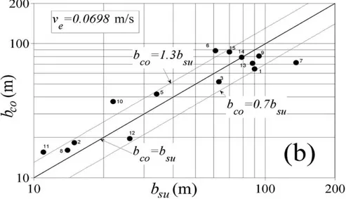
0.1022 m/s which obtained from applying the outlier-exclusion algorithm which suggested by Wahl (2004). The figures 2 and 3 show the comparison between the observed values of peak discharge and final average breach width with prediction results of the model of Macchione (2008) in predictive mode with applying average value of ve= 0.0698 m/s. The results of this study have been
Chapter 2 - The Macchione (2008) model 31
shown that the mean parameter of ve= 0.0698 m/s described very well the 12
Figure 2. Predicted peak discharge Qpc versus observed peak discharge Qps for earthen dam failures which considered in the study of Macchione (2008)
with ve=0.0698 m/s
Figure 3. Predicted breach average width bco versus observed one bsu for
earthen dam failures which considered in the study of Macchione (2008) with applying ve=0.0698 m/s
Table 1. Expressions for R, V, hc, dAb, dY, and l as Functions of Z and Y Breach R = V = l = Triangular Trapezoidal ℎ 𝛽 ℎ 𝑍 𝑍 𝛽 𝑍 𝑊 ℎ (ℎ ) ( 𝛽ℎ ) ℎ (ℎ )ℎ 𝑍 ( 𝑍 𝑍) 𝑍 𝛽 𝑍 𝑊 ℎ =
The temporal evolution of the variable Z is obtained by the continuity equation of volume W stored in the reservoir.
i ow
dW
Q Q Q
dt
(2.11)
in which Qi = inflow rate to the reservoir,
Qowsum of outflow dischargesthrough the outlet works; and Q= outflow discharge through the breach. To take the reservoir shape into consideration, the stored volume W is given as a function of Z by the level-reservoir volume curve, reported in what follows:
0
0
W
W Z
(2.12)
in which W0 coefficient and
0 actually varies between 1 and 4 (Marone, 1971). If Qi and
Qow are negligible with respect to Q, the continuity equation canbe expressed as: 0 1 0 0 dZ Z Q W dt
(2.13)
Moreover, the relation for discharge Q in the triangular breach and the trapezoidal breach is given by the following equations respectively:
5 2 1 2 1 4 ( ) tan 2 5 Q g ZY (2.14)
3 2 1 2 1 2 1 ( ) (h 2 ) (h Y) tan 2 c c c Q g h Y (2.15)
Chapter 2 - The Macchione (2008) model 35 0 1 0 0 5 2 1 2 5 2 4 ( ) ( ) ( ) tan 5 2 dZ g Z W Z Y dt
(2.16) 0 1 1 2 0 0 ( 2 ) (h 2 Y) h tan ( 0) 2( ) c c c c c g h Y dZ Z h Y dt W h Y
(2.17)
Therefore, the generation of outflow hydrograph in the first part of the phenomena (triangular breach) is calculated by equations (2.5) and (2.16) and the consequence discharge 𝑄 is given by Eq. (2.14). When the breach section becomes trapezoidal, the breach hydrograph is calculated by equations (2.5) and (2.17) and 𝑄 is given by equation (2.15). The initial conditions are given by the initial water level Z(0) in the reservoir and initial breach bottom elevation Y(0), at time t = 0.
36
Chapter 3
The power function for representing
the reservoir rating curve:
morphological meaning and
suitability for dam breach modeling
3.1
Introduction
Numerical computations concerning reservoirs, and in particular those that specifically have to describe filling and emptying processes, including those in dam breaching calculations, require the availability of information on the volume stored in the reservoir as a function of water depth. Since the reservoirs have a natural topography, their geometry cannot be expressed exactly by an analytical formula. For this reason, usually detailed tables are utilized for this purpose, where each value of elevation from bottom to top has a corresponding value for lake surface and reservoir volume. These tables very often are plotted and are known as elevation - volume or elevation - area curves. However, in the
Chapter 3 - Representing the reservoir rating curve 37
cases for which there is a scarcity of data, we have to interpolate the values of the table to achieve an analytical expression. Usually a polynomial function is the most appropriate one, but unfortunately it requires the assessment of several parameters and this may result in some difficulties in the systematic studies of flood control reservoirs or dam breach aimed at giving generalized solutions based on a number of characteristic parameters. In particular the systematic study of the dam breach problem is the reason which lead to this part of the research. As an example, if one wishes to develop the hydrograph computations using a non dimensional formulation, it is fundamental to decrease the number of parameters as much as possible. In this context the use of a polynomial function in the elevation-volume curve is not feasible. For this purpose, if applicable, it would be advantageous to express the reservoir rating curve, also called elevation-volume curve, using the power function, because this has the advantage of being a monomial function and only one parameter needs to be estimated. This expression has been already used in the past by other authors (Marone, 1971; Michels, 1977). Macchione (1986, 1989 & 2008), Macchione and Rino (2008) and De Lorenzo and Macchione (2011 & 2014) have used the power function in dam breach modelling for the calculation of flood hydrograph and peak discharge. However, some authors considered the use of this kind of expression an approximate approach (ASCE/EWRI, 2011). In this part of research, the high accuracy and suitability of this approach in representation of
the morphology of the reservoirs, at least for dam breach studies, have been shown. As a consequence, it will be shown that its use in numerical modelling does not affect the accuracy of calculations. This will be demonstrated in this part of thesis by analysing the suitability of the power function as an interpolating equation for reservoirs located in three different regions of the world, in order to verify the applicability of the function for various geological and geomorphological contexts. The results shown in the next sections can be found in (Macchione, et al., 2015).
3.2
Database used, investigation method and results
3.2.1 Database used
It is not easy to gather accurate surveys with a sufficient amount of data about the bathymetry of reservoirs from different regions of the world. Sometimes data are not open to the public and are not easily shared. However, on the Internet a very accurate database for many artificial reservoirs and dams from Texas is available at: http://www.twdb.texas.gov/surfacewater/58surveys /completed/list/
index.asp. Data available at this web site are the consequence of a survey
campaign carried out by the Texas Water Development Board (TWDB) started in 1991 for monitoring rates of sediment deposition in the reservoirs. The campaign included more than 100 reservoirs defined as “major reservoirs”; by definition, a major reservoir has a conservation storage capacity of 5000 acre −
Chapter 3 - Representing the reservoir rating curve 39
feet (6.2 ×10⁶ m3) or greater. Surveys have been replicated over the years, therefore more than one set of surveyed data may be available for some reservoirs. In order to have a bathymetry as close as possible to the early life of the reservoir, when more survey reports were available, the oldest has been considered for this study. The surveys were carried out with water level close to the top of conservation pool elevation, therefore for every dam, data are available up to this elevation. Technical details about criteria, tools and instruments used for the surveys can be found in the detailed reports available in the aforementioned web site. In these part of thesis, results of the surveys are shown in the tables “Reservoir volume table” or “Reservoir area table”. Volumes and areas are given in function of the elevation; each step in elevation is one tenth of a foot. In this analysis, in order to avoid the inclusion of reservoirs in which an abnormal sediment deposition occurred over time, the ones experiencing a loss of available volume larger than 20% since first filling have been ignored. Moreover off-channel reservoirs, reservoirs whose reports did not have the tables, or with missing or corrupt values for crucial data like crest elevation, have been excluded. In conclusion, 65 reservoirs have been considered eligible for the analysis (Macchione, et al., 2015). Fig. 4 shows how the reservoirs here analysed are characterized by very variegated shapes.
Chapter 3 - Representing the reservoir rating curve 41
This investigation also covers those technical situations for which high quality and very detailed tables, like the ones from TWDB, are not available. In particular, data about dams and reservoirs from Utah (USA), available at the web site of the Utah Division of Water Rights
http://www.waterrights.utah.gov/cgi-bin/damview.exe, have been analysed. In this case, only reservoirs having
enough data to cover all the aspects of the present analysis have been selected. Moreover, among these, only the ones having a hydraulic height greater than 10 m or having a stored volume greater than 106 m3 have been considered. As will be clear by the plots, the number of available points for each reservoir of the Utah database is much smaller if compared to TWDB reservoirs, except for one case which has a large number of points (BOR Jordanelle dam). From Utah we were able to find 18 reservoirs for this study. Finally, we have analysed 14 reservoirs in Calabria (Italy), having stored volumes greater than 106 m3 or a dam higher than 15 m. The interest in the study of reservoirs in these parts of the world lies in the fact that they belong to very different regions. Utah is a rocky region, but has almost three different geomorphological regions: the Rocky Mountains, the Great Basin, and the Colorado Plateau. Texas is a transition zone between the Great Plains and the Rocky Mountains; in this State plains, hills and plateau are the dominant landscape. Calabria is a narrow peninsula between the Tyrrhenian and the Ionian seas. Due to the morphological configuration of the land, the basins have a very limited extent and high slopes.
3.3
Verification of the suitability of the equation for the
description of the reservoir morphology
Data used in this study have been interpolated using the following equation:
0
0
W
W Z
(3.1)
Values of the terms W0 and
0 have been obtained by the least squares method. Table 2 shows the results of the investigation.Table 2. Reservoir considered in the analysis
As expected, average values of
0 have been found between 2 and 3. Moreover, higher values of
0 hardly exceed 4. The results are remarkable, concerning the quality of interpolation. Average values of R2 are close to 1 for each region.Therefore Eq. (3.1) is an excellent approximation for the elevation volume table. It can be also interesting to have a closer insight and check the adaptation of the power equation to the table as a function of the filling percentage in the reservoir. This analysis has been carried out for each region. The results are presented
Region N. of cases Av. α0 SQM α0 Min α0 Max α0 Av. R2 SQM R2 Min R2 Max R2
Texas 65 3.107 0.645 2.29 5.46 0.99942 0.000858 0.9941173 0.999983
Utah 18 2.71 0.588 1.75 3.917 0.998558 0.002668 0.989728 0.999996
Chapter 3 - Representing the reservoir rating curve 43
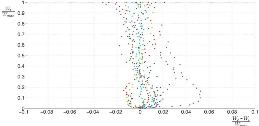
through some graphs in which the error 𝜖 is plotted versus the ratio Wt/Wmax,
where Wt is the volume read from the table for a given elevation and Wmax is the
maximum volume stored in the reservoir (Fig. 5 to 7). The parameter 𝜖 is the difference between the volume Wc computed by Eq. (3.1) and the surveyed one
Wt scaled to respect the maximum volume Wmax: max
c t
W W
W
(3.2)
multiplying 𝜖 by the ratio Wmax=Wt we obtain the local error that one gets by
using the curve in place of the table. So, in the Figures 5 to 7, the local error can be obtained by dividing the abscissa by the value of the ordinate. Figures 5 to 7 show that the error is very small throughout all the ordinate axis. For reservoirs of Texas the values are almost always in the range ±2% and so it is also for Calabria and Utah, although the amount of data available for those regions is smaller than the cases of Texas.
Chapter 3 - Representing the reservoir rating curve 47
3.4
Determination of parameters for elevation-volume curve
in limited data availability
Very often detailed data about reservoirs are missing or not readily accessible. Therefore, research studies or technical applications cannot rely on complete and reliable tables about elevations and the corresponding volumes, or lake area. In particular this situation is very common for dam breach studies concerning historical events. Very often lake area or stored volume are known only for few elevations, like conservation pool or maximum stored volume. It may be very interesting to know how accurate a volume-elevation curve obtained from a small number of points can be. If only two values of volume W1 and W2 are
available with the corresponding elevations Z1 and Z2, the values of W0 and
0 can be obtained by the following equations:1 0 1 2 2 log log logZ logZ W W
(3.3) 0 1 0 1 W W Z (3.4)If both the surface Sr and the volume Wr are known at the corresponding generic
elevation Zr, the value of
0 can be computed by (Macchione, 2008):0 r r r Z S W
(3.5)0 0 r r W W Z (3.6)
It may be very interesting to compute the error produced by these two methods for the calculation of W0 and
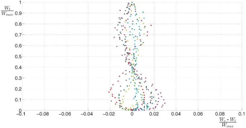
0. For this purpose, we have considered two elevations and their relative volumes and areas. The upper point was chosen at the normal pool level (highest elevation available), and the other one was chosen at a lower elevation. A sensitivity analysis has been carried out (Fig. 8-13), and the errors that are committed using different elevations for the lower point have been analysed. In particular the elevation of the lowest points was set in order to have a volume equal to 20%, 30%, 40%, 50% of the normal pool volume. Obviously, the error is nil in correspondence of the two selected points and has the maximum value in a certain point comprised between the selected points. The more is the distance between the selected points, the higher is the maximum error. The same is for the maximum error in the region between 0 and the lowest point. But in all the cases, the greatest values of errors are very low. Figures 8 to 10 show the results obtained setting the lowest point at 40% of the normal pool volume. The curves, whose parameters are calculated by Eq. (3.5) and (3.6), worsen more rapidly as the volume decreases (Fig 11-13); however, even for this method, the greatest values of error are almost always in the range ±5%. In the next section the suitability of the curve will be analysed for the dam breach problem.Figure 8. Error versus filling percentage of reservoirs from Texas database: interpolation based on two points only (the lowest one is located at 40% of normal pool level volume)
Figure 9. Error versus filling percentage of reservoirs from Utah database: interpolation based on two points only (the lowest one is located at 40% of normal pool level volume)
Figure 10. Error versus filling percentage of reservoirs from Calabria database: interpolation based on two points only (the lowest one is located at 40% of normal pool level volume)
Figure 11. Error versus filling percentage of reservoirs from Texas database: interpolation based on two points only (the lowest one is located at 30% of normal pool level volume)
Figure 12. Error versus filling percentage of reservoirs from Utah database: interpolation based on two points only (the lowest one is located at 30% of normal pool level volume)
Figure 13. Error versus filling percentage of reservoirs from Calabria database: interpolation based on two points only (the lowest one is located at 30% of normal pool level volume)
Chapter 3 - Representing the reservoir rating curve 55
3.5
Influence of the use of equation Eq. (3.1) on the outflow
hydrograph due to dam breach events
In order to assess the influence of the use of Eq. (3.1) on the outflow hydrograph due to the breaching of dams, a subset of only earthfill dams has been extracted from the reservoirs already studied in the previous sections. In particular, 50 earthfill dams have been extracted from the Texas database, 16 dams from the Utah database, and 6 dams from the Calabria database. For each dam the outflow hydrograph has been calculated using the model proposed by Macchione (2008). The same case studies have been simulated introducing a slight modification to the model that allows the direct use of the surface-elevation table. In particular
S(h) has been used in place of W(h) as in the mass conservation equation of the
model we find the derivative dW/dZ and not actually the volume, and as said in the previous sections dW/dZ is the lake area at elevation Z. In order to assess the suitability of Eq. (3.1) in the approximation of the volume-elevation table on the outflow hydrograph, the differences between the values of some variables computed using the methods shown in the previous section have been calculated. In particular the peak discharges Qp, W, the time to peak discharge Tp and the
final average breach width Bm have been compared. Tables 3 to 8 show average
values, maximum values and standard deviations. Moreover the average value of parameter R2 reported in those tables, show the level of accuracy provided by the analysed interpolation methods.
Table 3. Method of interpolation: least square of all elevation-volume data
Table 4. Method of interpolation: Eq. (3.5) and Eq. (3.6)
Texas 15 0.999567 0.000537 0.999983 0.996985 1.062 1.910 0.684 1.262 0.438 0.739 0.333 0.647
Utah 16 0.999996 0.000701 0.997594 0.999416 0.235 1.140 -0.764 1.239 -1.562 3.122 -0.889 1.462
Calabria 6 0.999494 0.000438 0.999722 0.998603 0.799 2.143 0.292 1.328 -0.403 0.844 0.110 0.745
Wgt. Avg 0.999656 0.856 0.33 -0.076 0.0429
Min R2
Region N. Cases Avg. R2 SD R2 Max. R2 Avg. 𝑄 SD Avg. SD Avg. SD Avg. SD 𝑄 𝑄 𝑄 𝑊 𝑊 𝑊 𝑊 Texas 50 0.997193 0.99409 0.999941 0.97793 0.026 1.543 0.002 0.425 -0.257 2.004 -0.116 0.49 Utah 16 0.995797 0.003484 0.999965 0.990391 -1.037 1.012 -0.048 0.681 -3.258 3.148 -1.384 1.521 Calabria 6 0.995944 0.003776 0.999637 0.989154 -1.033 0.752 0.141 0.445 -1.403 1.400 -0.306 0.536 Wgt. Avg 0.996778 -0.298 0.002 -1.019 -0.414 SD
Region N. Cases Avg. R2 SD R2 Max. R2 Min R2 Avg. 𝑄 SD Avg. SD Avg. Avg. SD 𝑄 𝑄 𝑄 𝑊 𝑊 𝑊 𝑊