Wind turbine simulator fault diagnosis via fuzzy modelling and identification techniques

Contents lists available atScienceDirect

Sustainable Energy, Grids and Networks

journal homepage:www.elsevier.com/locate/segan

Wind turbine simulator fault diagnosis via fuzzy modelling and

identification techniques

Silvio Simani

a,∗

, Saverio Farsoni

a

, Paolo Castaldi

b a_{Department of Engineering, University of Ferrara, Ferrara, FE. 44122, Italy} b_{Electric and Informatics Department, University of Bologna, Bologna, Italy}

a r t i c l e i n f o

Article history:

Received 21 September 2014 Received in revised form 18 December 2014 Accepted 23 December 2014 Available online 9 January 2015

Keywords:

Fuzzy modelling and identification Fault detection and isolation Residual generators Sustainability and availability Wind turbine benchmark

a b s t r a c t

For improving the safety and the reliability of wind turbine installations, the earliest and fastest fault detection and isolation are highly required, since it could be used also for accommodation purpose. Modern wind turbines consist of several important subsystems, which can be affected by malfunctions regarding actuators, sensors, and components. From the turbine control point-of-view they are extremely important since provide the actuation signals, the main functions, as well as the measurements. In this paper, a fault diagnosis scheme based on the identification of fuzzy models is described, in order to detect and isolate these faults in the most efficient way, in order also to improve the energy cost, the production rate, and reduce the operation and maintenance operations. Fuzzy systems are proposed here since the model under investigation is nonlinear, whilst the wind speed measurement is uncertain since it depends on the rotor plane wind turbulence effects. These fuzzy models are described as Takagi–Sugeno prototypes, whose parameters are estimated from the wind turbine measurements. The fault diagnosis methodology is thus developed using these fuzzy models, which are exploited as residual generators. The wind turbine simulator is finally employed for the validation of the obtained performances.

© 2015 Elsevier Ltd. All rights reserved.

1. Introduction

Modern industrial processes and controlled plants can exploit many technical resources comprising for example information sciences, real-time solutions, advanced diagnosis and control, and computational intelligence. This paper aims at reporting recent developments in the emerging areas of technology that find applications to factory advanced control and diagnosis, such as wind turbine installations.

The control tools normally used for improving the complete behaviour of power plants can exploit both advanced control schemes and complicated hardware solutions (for example, smart sensors, virtual actuators and processing units). This high com-plexity degree can increase the failure rate, thus motivating the requirement of an automatic scheme employed to quickly diag-nose any abnormal working situations. These remarks raised a great interest in the issues of Fault Detection and Isolation (FDI) for dynamic systems, and many model-based strategies were sug-gested, as described for example in [1–4]. These methods rely on

∗_{Corresponding author.}

E-mail address:silvio.simani@unife.it(S. Simani).

URL:http://www.silviosimani.it(S. Simani).

the mathematical description of the process under diagnosis. How-ever, the diagnosis principle can be based on a limited number of approaches, i.e.: the parity space method, the state or output esti-mation, the Unknown Input Observer (UIO) principle, the Kalman Filters (KF) tool, the Unknown Input Kalman Filters (UIKF) strategy, and the parameter identification approach. Moreover, techniques relying on the artificial intelligence tools were also proposed [5]. Even if several linear and nonlinear methodologies were proposed, robust and reliable (in one word, ‘‘sustainable’’) FDI requires future researches.

It is worth noting that the accurate detection and isolation of faults can require a precise mathematical description of the plant under diagnosis, which can be expressed as state-space or in-put–output formulation. In this way, after the generation of the residual signals, their evaluation should guarantee the accurate fault detection, while avoiding the indication of false alarms gen-erated by disturbance, measurement errors, and the model-reality mismatch. However, in actual conditions, the direct design and ap-plication of these FDI approaches can be difficult, motivated by the complexity of the mathematical description involved. This un-avoidable complexity cannot allow the direct use of most of the linear FDI schemes, thus requiring a viable strategy for the direct application of the diagnosis schemes to practical examples [3,6]. http://dx.doi.org/10.1016/j.segan.2014.12.001

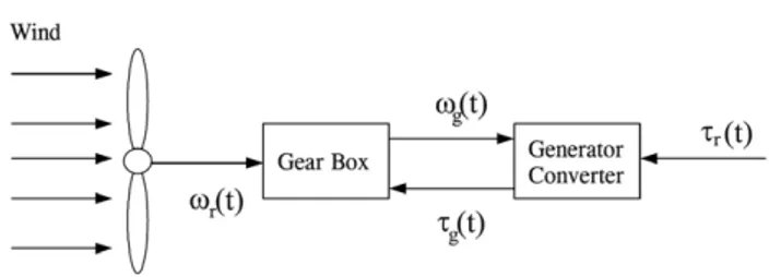
Fig. 1. Wind turbine schematic diagram.

With reference to wind turbines, as considered in this work, many papers considered the model-based FDI problem [7,8]. They showed that the more accurate the representation is at modelling the plant dynamics, the better its behaviour will be in diagnosing abnormal working situations.

This paper proposes the use of the fuzzy modelling and identifi-cation tool with appliidentifi-cation to a wind turbine benchmark for deter-mining a straightforward solution of the FDI task. Two key issues of the proposed study are remarked. First, the model complexity does not imply the need of a complex mathematical description. In fact, as described here, the fuzzy modelling and identification tool can be exploited, thus avoiding purely nonlinear equations. Moreover, the mathematical description of the residual generators is derived via an identification approach. On the other hand, fuzzy prototypes as residual generators are designed, rather than purely nonlinear filters. This aspect is quite important when the designed diagnosis tool is proposed for real-time solutions. Moreover, the diagnosis scheme proposed in this study paper will be analysed in compar-ison with different approaches relying e.g. on banks of UIO/KF, as described in [1,3].

This work proposes the use of the fuzzy logic theory, since it seems to be a simple tool able to manage complicated and un-known situations [9]. In particular, the residual generators ap-plied to the wind turbine benchmark are derived as Takagi–Sugeno (TS) fuzzy descriptions [10], whose parameters are estimated via a system identification strategy. The efficacy of the suggested approaches are verified on the wind turbine benchmark mea-surements. Real-time simulations comprising realistic fault and working situations are used to assess the efficacy of the suggested methodologies.

It is worth noting that, with respect to the previous work by one of the same authors [11], this paper extends the results and improves the efficacy of the proposed solution. On the other hand, the identification approach, which is extended to the fuzzy frame-work and applied to the wind turbine data in this study, was devel-oped by one of the same authors in [12]. Moreover, the design of the fuzzy estimators, which in this paper is exploited for the fault isolation task, was described in a paper by the same author [13], but applied to a diesel engine system.

Finally, the paper has the structure as detailed below. Section2

addresses the wind turbine model exploited in the work. Section3

describes the fuzzy modelling and identification tool used for FDI strategy development. The suggested FDI scheme is considered in Section4. The obtained results reported in Section5serve to highlight the efficacy of the fuzzy tool, which is compared also with respect to a different FDI scheme. Section6concludes the work by summarising the main points of the paper and suggesting some future research issues.

2. Wind turbine simulated model

The paper considers a realistic wind turbine with horizontal axis and three blades that move the rotor shaft due to the incoming wind flow. A gear-box is used for up-scaling the rotational speed of the power generator. More details of this benchmark wind turbine

are available in [7]. Fig. 1provides the diagram of this power plant.

The converter torque

τ

g

(

t

)

and the turbine blade pitch angle

β

r

(

t

)

are the two control inputs used to regulate the rotational

speed

ω

r

(

t

)

and the generated power Pg

(

t

)

. On the other hand,

ω

g

(

t

)

represents the generator speed, whilst

τ

g

(

t

)

is generator

torque depending on the converter torque reference,

τ

r

(

t

)

.

τ

aero

(

t

)

is the aerodynamic torque, whose estimate is computed from the wind speed,

v(

t

)

. However, this measurement is very uncertain, as shown e.g. in [7].

The aerodynamic description is provided by Eq.(1):

τ

aero

(

t

) =

ρ

A Cp

(β

r

(

t

), λ(

t

)) v

3

(

t

)

2

ω

r

(

t

)

(1) with the air density

ρ

, the turbine blade area A, the reference pitch angle

β

r

(

t

)

, and the tip–speed ratio

λ(

t

)

, described by Eq.(2):

λ(

t

) =

ω

r

(

t

)

R

v(

t

)

(2)

where the rotor radius is R. With reference to Eq.(1), the term Cpdescribes the power coefficient that is usually represented by

a two-dimensional map. Since the wind speed measurement

v(

t

)

is uncertain, it is assumed that

τ

aero

(

t

)

is affected by an error, which

justifies the proposed approach of Section3. The proposed scheme is also able to manage the nonlinearity described by the expres-sions of Eqs.(1)and(2).

The drive-train is described as a one-body model and the complete hydraulic pitch system is modelled as a second or-der transfer function [7]. Under these hypotheses, the overall continuous-time state-space model of the wind turbine process is described by Eq.(3):



_˙

_x

c

(

t

) =

fc

(

xc

(

t

),

u

(

t

))

y

(

t

) =

xc

(

t

)

(3) where the available control inputs are represented by the vector u

(

t

) = β

1 mi

(

t

), β

2 mi

(

t

), β

3 mi

(

t

), τ

g

(

t

)

T

and the output mea-surements are described by the vector y

(

t

) =

xc

(

t

) = 

Pg

(

t

),

ω

g mi

(

t

), ω

r mi

(

t

)

T

, respectively. These measurements are pro-vided by two redundant sensor signals, with i

=

1

,

2. The static function fc

(·)

describes the nonlinear relation between inputs and

outputs. As described in Section3, this nonlinear system will be approximated using the fuzzy models estimated from N data se-quences u

(

k

)

and y

(

k

)

, where k

=

1

,

2

, . . . ,

N, are the sampling intervals.

With reference to the available redundant measurements from the benchmark,

ω

g miand

ω

r mi represent the generator and rotor

speed signals, respectively.

β

j mi

(

t

)

refers to the ith measurement

of the jth blade pitch. The look-up table Cp

(β, λ)

is selected for

describing a high-fidelity wind turbine, which is the test-rig for the validation of the proposed approach.

Finally, the measurement errors are described as Gaussian processes with statistics that represent realistic wind turbine measurement sensors.

2.1. Fault mode and effect analysis

The benchmark system considered in this paper simulates a number of realistic faults, described inTable 1, which represent typical malfunctions of wind turbine installations. More details are available in [7].

In order to simplify the approach to the FDI task, the links between the fault situations reported above and the considered wind turbine measurements were considered and analysed.

Table 1 Fault scenario.

Fault Description

1 Position sensor 1 of the pitch 1: stuck value 2 Position sensor 2 of the pitch 2: scaled value 3 Position sensor 1 of the pitch 3: stuck value

4 Rotor speed sensor 1: stuck value

5 Rotor speed sensor 2 & generator

speed sensor 2: scaled values

6 Pitch 2 actuator: changed dynamics due to

air content in the hydraulic circuit

7 Pitch 3 actuator: changed dynamics due to

hydraulic circuit low pressure

8 Converter torque control: offset value

9 Drive train: changed dynamics

Table 2

Results of the FMEA approach.

Measurements Fault β1 m1(t) 1 β2 m2(t) 2 β3 m2(t) 3 β1 m2(t) 4 β2 m1(t) 5 ωr m1(t) 6 ωr m2(t) 7 Pg(t) 8 ωr m1(t) 9

Therefore,Table 2summarises the effects of the single faults on the inputs u

(

k

)

and outputs y

(

k

)

signals acquired from the simulated process.

The results reported inTable 2were achieved by using the so-called Failure Mode & Effect Analysis (FMEA) [14]. In particular,

Table 2shows the most sensitive input u

(

k

)

or output y

(

k

)

mea-surement with reference to the considered fault situations. Obvi-ously, fault conditions different from the ones considered in this paper could probably require different measurements. The ap-proach is similar to the procedure shown in [13,12], and it repre-sents an important key point, since it simplifies the fault isolation task, described in Section4, and the set of measurement inputs and outputs to be used for identification purpose, recalled in Section3.

3. Fuzzy modelling and identification

This section addresses the derivation of the residual generators used for the wind turbine benchmark FDI. In particular, the param-eter estimation method summarised in the following enhances the development of the suggested FDI scheme reported in Section4.

The TS fuzzy prototype consists of a set of rules Ri, where the

consequents are deterministic functions fi:

Ri

:

IF x is AiTHEN yi

=

fi



x



(4)

where i

=

1

,

2

, . . . ,

K , with K the number of rules (or clusters). The term x describes the antecedent variables, whilst yirepresents

the consequent outputs. The fuzzy set Aiof the ith rule is

repre-sented with a (multivariable) membership function, as described e.g. in [9].

The terms fiare properly parametric models, whose structure is

fixed, and only its parameters can vary. These functions exploited in this study have the affine form of Eq.(5):

yi

=

aix

+

bi

,

(5)

with aiand birepresent the model parameters. These models are

proposed in this study as they are able to approximate nonlinear systems with an arbitrary degree of accuracy [15].

When the degree of fulfilment of the antecedent

λ

i

(

x

) =

µ

Ai

(

x

)

is computed, the complete TS model is represented with the

expression: y

=

K



i=1

λ

i

(

x

)

yi K



i=1

λ

i

(

x

)

(6)

where the membership functions

λ

iare usually described with

ex-ponential functions [9]. Section5will show that exponential mem-bership functions represent the optimal choice for the accurate description of the fuzzy cluster shapes.

It is worth noting that the TS model of Eq.(4)can approximate a dynamic system if the consequents are described as linear autoregressive models x

(

k

) = [

y

(

k

−

1

), . . . ,

y

(

k

−

n

),

u

(

k

−

1

),

. . . ,

u

(

k

−

n

)]

T, and ai

= [

α

1(i)

, . . . , α

(i) n

, δ

(1i)

, . . . , δ

(i) n

]

, with n is

the memory (order) of the system. When the structure of Eq.(6)is considered, a methodology developed in [16] is exploited for the identification of both ai, bi, and the model order n.

On the other hand, the membership degrees

λ

i of Eq.(6)are

easily estimated using the fuzzy clustering procedure described in [9]. In particular, this work proposes to use the fuzzy c-means clustering method developed in [9] and already available as ready-to-use program. Moreover, this clustering tool choice is that it can be directly integrated with the estimation scheme suggested by one of the authors in [16]. The issue of the estimation of the optimal number of clusters K was considered e.g. in [16,17].

The remaining part of this section summarises the procedure for the estimation of the TS fuzzy model parameters from noisy data.

Several techniques for the estimation of the model parameters aiand biin Eq.(5)are available. However, if it is assumed that errors

affect both the regressor and the regressand variables, the optimal parameters are identified by exploiting a scheme known as Errors-In-Variables (EIV) approach [18]. In fact, it can be considered here since it leads to the minimisation of the estimation (or prediction) errors of the K independent local affine models [17].

To this aim, with reference to the ith cluster (i

=

1

, . . . ,

K ), the data matrices are built as follows:

X_n(i)

=











y

(

k

)

xT_n

(

0

)

1 y

(

k

+

1

)

xT_n

(

1

)

1

...

...

y

(

k

+

Ni

−

1

)

xTn

(

Ni

−

1

)

1











(7)

with n representing the number of delayed inputs and outputs, i.e. xn

(

h

) = [

y

(

h

−

1

), . . . ,

y

(

h

−

n

),

u

(

h

−

1

), . . . ,

u

(

h

−

n

)]

T. Moreover:

Σ(i)

n

=



X_n(i)



TX_n(i)

.

(8)

The problem of noise rejection is thus solved with the assumption that the measurement noise represented by the signalsu

˜

(

k

)

and

˜

y

(

k

)

are additive on the input and output measurements u∗

₍

_k

₎

_and y∗

₍

_k

₎

_{, with a number of sampling instant k}

₌

₁

_,

₂

_{, . . . ,}

_{N. In this}

situation, the positive-definite covariance matrixΣn(i) related to

the data of the ith cluster can be described as the contribution of two addenda, that isΣn(i)

=

Σ

∗(i) n

+

Σ

¯˜

n.

In particular, the covariance matrixΣ

¯˜

nhas the form:

¯˜

Σn

=

diag

[ ¯˜

σ

yIn+1

, ¯˜σ

uIn

,

0

] ≥

0

.

(9)

This identification problem is solved by computing the unknown noise variance values

σ

¯˜

uand

σ

¯˜

ythat derive from Eq.(10):

Σ∗₍i)

n

=

Σ(

i)

which is a function of the unknowns

σ

˜

_u and

σ

˜

_y and Σ

˜

n

=

diag

[ ˜

σ

_yI_n+1

, ˜σ

uIn

,

0

]

. Actually, the parameters of the local affine

model are estimated by determining the noise variances

( ˜σ

u

, ˜σ

y

) ∈

Γ(i)

n+1

=

0 making the matrixΣ

∗₍i)

n+1 close to the double singular

condition. However, in each ith cluster, different noise variances

( ¯˜σ

(ui)

, ¯˜σ

(i)

y

)

are assumed, and the following expression is derived:

Σ∗₍i) n

=

Σ( i) n

− ˜

Σ( i) n

≥

0 (11) withΣ

˜

n(i)

=

diag

[ ¯˜

σ

(i) uIn+1

, ¯˜σ

(i) y In

,

0

]

. The values

( ¯˜σ

(i) u

, ¯˜σ

(i) y

)

repre-sent the additive noise variance values of the data in the ith cluster. These assumptions mean that the following relations normally hold [19,16]:



u

(

k

) =

u∗

(

k

) + ˜

u

(

k

)

y

(

k

) =

y∗

(

k

) + ˜

y

(

k

)

(12)

where u∗

₍

_k

₎

_{and y}∗

₍

_k

₎

_{represent the data without noise, whilst}

the noise signals u

˜

(

k

)

and y

˜

(

k

)

do not depend on other terms. Moreover, only the measurements u

(

k

)

and y

(

k

)

are available.

Finally, the matrices_Σ

˜

(i)

n are derived and the model parameters

for the ith cluster are estimated via the expression:



Σ(i) n

− ˜

Σ( i) n



a(i)

=

0 (13)

with i

=

1

, . . . ,

K , and a number of K clusters. This identification approach will be exploited for the estimation of the residual generators for FDI as described in Section4.

4. Fault diagnosis strategy

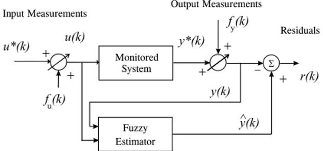
The issue of the residual generator design for the FDI of the wind turbine model will be addressed in this section.

The wind turbine system is assumed to be modelled by the description of Eq. (3). u

(

k

)

and y

(

k

)

represent the controlled inputs and the system outputs, respectively. The so-called model-reality mismatch in fault-free conditions can be represented by the difference y

(

k

) − ˆ

y

(

k

)

. It could take into account measurement errors, parameter variations, and disturbance. The reconstruction of the measurement y

(

k

)

, i.e.

ˆ

y

(

k

)

is obtained from an identified model of Eq.(6). According to the description of Eq.(12), in practice, the signals u∗

₍

_k

₎

_{and y}∗

₍

_k

₎

_{are acquired by measurement sensors,}

which are inevitably affected by errors.

On the other hand, if the sensor dynamics are neglected, also faults affect the measurement process, which is thus modelled as:



u

(

k

) =

u∗

(

k

) +

fu

(

k

)

y

(

k

) =

y∗

(

k

) +

fy

(

k

)

(14) where the terms fu

(

k

)

and fy

(

k

)

are additive fault signals.

Regarding the FDI task, this paper proposed to use TS fuzzy prototypes that are exploited for residual generators from the redundant input and output signals u

(

k

)

and y

(

k

)

. In this way,Fig. 2

shows that proper residual signals are computed as:

r

(

k

) = ˆ

y

(

k

) −

y

(

k

)

(15)

i.e. the difference between the actual y

(

k

)

and its reconstruction

ˆ

y

(

k

)

.

After the residual generation task, its evaluation is performed for detecting any fault occurrence, and for isolating the faulty actuator or sensor signals.

A direct geometric threshold comparison is proposed here to perform the fault detection stage. However, a detection delay can be present due to the fault modes summarised in Section2.1. The

Fig. 2. The generation of the residual signals for FDI.

fault detection logic is performed according to the test described by Eq.(16):











¯

r

−

δ σ

_r

≤

r

(

k

) ≤ ¯

r

+

δ σ

_r if fault-free r

(

k

) < ¯

r

−

δ σ

_r or r

(

k

) > ¯

r

+

δ σ

_r if faulty

.

(16)

Actually, the residual r

(

k

)

is modelled as a stochastic variable, whose mean and variance values are estimated with the relations of Eq.(17):



















¯

r

=

1 N N



k=1 r

(

k

)

σ

2 r

=

1 N N



k=1 [r

(

k

) − ¯

r]2 (17)

where the termsr and

¯

σ

2

r represent the mean and variance values

of the fault-free residual samples, respectively. In Eq. (17)the sample number of r

(

k

)

is N. Note thatr and

¯

σ

2

r could be exactly

computed from the r

(

k

)

statistics, usually unknown.

A robustness and reliability degree is introduced for distin-guishing the normal and the faulty behaviours, which is repre-sented by the tolerance parameter

δ

(normally

δ ≥

2). A technique developed in [20] by one of the same authors is applied here not to obtain conservative results. In particular, extensive simulations lead to the optimal value of

δ

that minimises the false alarm prob-ability and maximise the true detection rate. This topic will be fur-ther analysed in Section5.

The second issue concerns the fault isolation task, and it is achieved using a bank of residual generators properly designed, which resembles the Generalised Observer Scheme (GOS) [1]. This task can be easily solved here as Section2.1showed how different faults fy

(

k

)

or fu

(

k

)

affect different input or output measurements.

In this way, when the outputs are fault-free, fu

(

k

)

possibly affecting

one of the inputs u

(

k

)

, is diagnosed with a bank of TS fuzzy estimators of Eq.(6), as depicted inFig. 3.

The number of residual generators coincides with the number of faults to be diagnosed. Fig. 3 shows that the ith residual generator is fed by all but the ith input measurement (or even more input signals, if necessary) and all output measurements. The generated residual signal is thus sensitive to all but the ith fault fu

(

k

)

. These residual generators are described by fuzzy TS

models that are identified with the strategy reported in Section3. In particular, the ith fuzzy estimator that does not depend on the ith input measurement is identified using y

(

k

)

and all but the ith input measurement ui

(

k

)

(i

=

1

, . . . ,

r).

On the other hand, when the input variables are fault-free, a fault fy

(

t

)

affecting the output measurement is diagnosed with an

output fuzzy estimator bank, which are organised as inFig. 3. The efficacy of the overall fault isolation scheme is summarised inTable 3, where the so-called ‘‘fault signatures’’ are summarised for the single fault case regarding each input–output signal. It is worth noting that the residuals riofFig. 3are indicated by rIi or

Fig. 3. Scheme for the isolation of input faults. Table 3 Fault signatures. u1 u2 . . . ur y1 y2 . . . ym rI1 0 1 . . . 1 1 1 . . . 1 rI2 1 0 . . . 1 1 1 . . . 1 .. . ... ... ... ... ... ... ... ... rIr 1 1 . . . 0 1 1 . . . 1 rO1 1 1 . . . 1 1 0 . . . 0 rO2 1 1 . . . 1 0 1 . . . 0 .. . ... ... ... ... ... ... ... ... rOm 1 1 . . . 1 0 0 . . . 1

rOiinTable 3if they are generated by the bank for input or output

sensor fault isolation, respectively.

With reference toTable 3, an entry ‘1’ means that the residual is affected by the fault, whilst ‘0’ indicates that the corresponding residual does not depend on the particular fault.

Finally, according toTable 3, it is worth noting that multiple faults are isolable, as only the ith output signal feeding the residual generator of rOi is affected by the fault on yi. On the other hand,

multiple faults on the inputs uiare not isolable as the residuals rIi

depend on the faults affecting different inputs.

5. Simulated results

The suggested identification and FDI approach was applied to the benchmark summarised in Section2. The data exploited for identification purpose were N

=

440

×

103_{samples acquired with}

a sampling rate of 100 Hz.

5.1. Wind turbine modelling and FDI

As addressed in Section3, the data clustering algorithm with K

=

4 fuzzy sets and n

=

2 was employed. After this fuzzy c-means clustering, the residual generator parameters ai and bi

(i

=

1

, . . . ,

K ) were identified according to Section3. In particular,

Fig. 3highlighted that the residual signals for FDI were computed using a bank of 5 TS fuzzy estimators of Eq.(6).Table 2suggested that this approach is able to diagnose the faults 1–5, according to

Fig. 3. Moreover, by following again the results ofTable 2, a bank

Fig. 4. The signalsyˆ(k)andyˆ(k)for fault 4.

Fig. 5. The residuals rIi(t)for fault 4.

of 4 fuzzy residual generators allowed the diagnosis of the faults 6–9. Note that the membership functions

β

iused in Eq.(6)were

estimated as Gaussian functions, and derived from the same fuzzy c-means clustering approach [21].

In the following, the simulation results regarding fault 4, i.e. fu

(

t

)

, commencing at the instant t

=

1500 s are shown. Moreover,

fault 8 corresponding to fy

(

t

)

is also presented. This fault is active

between the time instants 3800 and 3900 s. These faults change the measurements u

(

t

)

and y

(

t

)

, and therefore affect the residuals rIi

(

t

)

generated by the residual generator of Eq.(6). These residual

signals are compared with fixed thresholds according to Eq.(16). As an example,Fig. 4shows the fault-free y

(

k

)

(grey dashed line) and the faultyy

ˆ

(

k

)

(black continuous line) signals regarding the

ω

r

(

t

)

measurement from the device ofFig. 2. On the other hand,

Fig. 5compares the corresponding fault-free residual rIi

(

t

)

(grey

dashed line) with the corresponding faulty one (black continuous line) generated by the device ofFig. 3.

Fig. 5also depicts the FDI thresholds of Eq.(16)using dotted constant lines. In the following, a simulation tool will be described for determining their values in order to minimise both the false alarm rate and the missed fault probability, as well as to maximise the correct FDI rates. Therefore, the diagnosis of the considered faults is correctly performed if the corresponding residuals exceed these thresholds, as shown inFig. 5.

With reference to fault 8, i.e. fy

(

t

)

considered here,Fig. 6shows

the fault-free y

(

k

)

(grey dashed line) and the faultyy

ˆ

(

k

)

(black continuous line) signals concerning the

τ

g

(

t

)

measurement from

the device ofFig. 2.

On the other hand,Fig. 7depicts the fault-free residual with grey dashed line and the faulty residual in black continuous line.

Also in this case,Fig. 7reports also the FDI thresholds as dotted constant lines. They were optimally selected in order to achieve the minimisation of the false alarm rate and the missed fault probability. Note that the obtained results show the efficacy of the proposed FDI methodology relying on fuzzy residual generator functions identified from uncertain measurements generated by the wind turbine benchmark.

Fig. 6. The signals y(k)andˆy(k)for fault 8.

Fig. 7. The residual signals rOi(t)for fault 8.

Table 4

FDI features of the UIKF bank.

Fault Fault isolation FDI delay (s)

1 Yes 15.98 2 Yes 95.89 3 Yes 20.61 4 Yes 10.34 5 Yes 91.14 6 No 55.71 7 No 55.65 8 No 18.98 9 No 12.68 5.2. FDI comparisons

This section reports the comparison of the proposed strategy with respect to a different FDI approach. In particular, the features of the FDI method developed in this study are analysed by con-sidering an Unknown Input Kalman Filters (UIKF) bank proposed e.g. in [1]. These UIKF devices used as residual generators were ob-tained from a linear state-space description of the wind turbine benchmark, and designed as described e.g. in [22,23]. However, the fuzzy multiple-model identification was not exploited here. The achieved results are summarised inTable 4, which reports if the considered faults are isolable and their FDI delays.

With reference to the results of Table 4, note that model-based schemes should be used if accurate descriptions of the process models are available. Moreover, the UIKF solution can manage the disturbance rejection problem by exploiting complex design algorithms. However, Table 4shows that the UIKF fault sensitivity is lower than the fuzzy predictors. On the other hand, the advantage of the proposed fuzzy approach relies on its simplicity, even if a suitable FDI threshold selection procedure can be required, as sketched in the remaining part of this section. 5.3. FDI performance evaluation

To this aim, further simulations are shown for achieving the optimal performance and evaluating the features of the proposed FDI scheme with reference to the model-reality mismatch and the measurement errors. Thus, extensive experiments were realised by

Table 5

Monte-Carlo analysis with the fuzzy estimators.

Fault FAR MFR TFDIR MFDID (s) δ

1 0.002 0.003 0.997 0.03 3.8 2 0.001 0.001 0.999 0.47 4.3 3 0.002 0.003 0.997 0.06 4.2 4 0.002 0.003 0.997 0.04 4.5 5 0.001 0.001 0.999 0.03 3.7 6 0.002 0.003 0.997 0.73 4.4 7 0.002 0.003 0.997 0.61 4.3 8 0.001 0.001 0.999 0.03 3.5 9 0.002 0.003 0.998 0.15 3.9

using the wind turbine simulator of Section2the Monte-Carlo tool. In fact, this methodology is extremely powerful here since the FDI effectiveness is a function of the residual signals sensitivity with respect to the model uncertainty and the measurement accuracy.

Section4highlighted that the input and output sequences u

(

k

)

and y

(

k

)

can be generated with arbitrary measurement errors and noise levels. Therefore, the evaluation of the achievable perfor-mance is based on properly computed indices, which were mo-tivated by previous studies, see e.g. [24,25]. They were evaluated using 1000 Monte-Carlo simulations, and empirically computed as:

•

False Alarm Rate (FAR): the ratio between the number of wrongly detected faults and the number of simulated faults;

•

Missed Fault Rate (MFR): the ratio between the total number of

missed faults and the total number of considered faults;

•

True FDI Rate, (TFDIR): the ratio between the number correctly

diagnosed faults and the total number of occurred faults;

•

Mean FDI Delay, (MFDID): the average FDI delay interval.

Table 5reports the evaluation of these indices when the fuzzy predictors proposed here are considered and the optimal

δ

in Eq.(16)was selected.

Table 5highlights that the optimal values of

δ

in Eq.(16)allow to obtain FAR and MFR values lower than 0

.

3%, with TFDIR larger than 99

.

7%, with minimal MFDID times. This aspect represents one of the key issues of the suggested strategy, which demonstrates the efficacy of the Monte-Carlo tool exploited here for the evaluation of the robustness issue of the suggested methodology. The simulation tests seem to be also able to enhance the designer to assess the reliability feature of designed FDI strategy when applied to more realistic examples.

5.4. Hardware-in-the-loop experiments

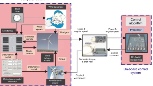
For the evaluation of more realistic working conditions, since real data from a wind turbine are not available, this section sum-marises the results achieved using an Hardware In the Loop (HIL) setup. The procedure serves also to highlight the performance of the designed software algorithms realising the proposed FDI strat-egy and working in an real-time conditions when implemented on-board the wind turbine installation.Fig. 8describes the schematic diagram of the HIL test-rig.

This test-rig was already presented in [11] but for control per-formance evaluation. The setup consists of an industrial computer that provides the modelling of the wind turbine dynamics in the Labview⃝R _{environment. The FDI strategy suggested in this study} was implemented using the AWC 500 system with its on-board electronics and interface circuits, which simulate the data acqui-sition and transmission processes.Table 6summarises the results obtained using this real-time laboratory setup.

Table 6highlights the consistency of the almost real-time tests with respect to the results shown inTable 5from the Monte-Carlo simulation tool. In fact, note that the performances ofTable 5seem to be better than the HIL tests inTable 6. However, the numerical

Fig. 8. Main elements of the HIL test-bed. Table 6

HIL laboratory setup FDI results.

Fault FAR MFR TFDIR MFDID(s) δ

1 0.005 0.005 0.995 0.07 4.1 2 0.004 0.004 0.996 0.49 4.5 3 0.004 0.004 0.996 0.08 4.6 4 0.005 0.005 0.995 0.07 4.8 5 0.003 0.004 0.997 0.06 3.9 6 0.004 0.005 0.996 0.76 4.8 7 0.005 0.004 0.995 0.64 4.5 8 0.005 0.004 0.995 0.06 3.8 8 0.004 0.005 0.996 0.18 4.3

implementation precision of the on-board processor and the signal processing electronics motivate possible deviations between the achieved results, which seem quite accurate when almost real-time wind turbine experimental applications are experimented with.

Finally, note that the main challenge in this application area is to reduce the energy cost allowed by the presented fault diagnosis strategy, without significantly increasing the cost of the installa-tion operainstalla-tions. In this way, the cost of the energy can be decreased by about 2%, mainly due to an increase in the system reliability. Furthermore, the wind turbine availability will be increased corre-spondingly, by the features of the diagnosis scheme developed in the paper, which allows to achieve the objective of decreasing lost production factor by 10%. This thus leads to an impact on increas-ing the attractiveness of the wind turbine technology by improvincreas-ing the cost and increasing reliability and availability.

6. Conclusion

This paper suggested a viable approach for the development of a fault diagnosis scheme with application to a wind turbine benchmark. The scheme relies on fuzzy prototypes that are iden-tified from uncertain input–output data measurements. The pro-cess under diagnosis is nonlinear and the acquired measurements are affected by errors due to the wind speed uncertain knowledge. These identified fuzzy models were used for robust residual gener-ation. The estimation procedure used for deriving the fuzzy model parameters exploited a data fuzzy clustering tool and a system identification algorithm solving the noise-rejection problem. The efficacy of this approach was investigated also in real-time condi-tions and comparisons with a different fault diagnosis highlighted the key features of the proposed methodology. In this way, by con-sidering wind turbine standard installations, with typical costs and

production rates, the fault diagnosis scheme presented here could be able to reduce the lost production factor with at least 10%, and to decrease the cost of energy by 2%, due to the decrease of unex-pected and unplanned maintenance operations, representing the most expensive costs for wind turbines.

References

[1]J. Chen, R.J. Patton, Robust Model-Based Fault Diagnosis for Dynamic Systems, Kluwer Academic Publishers, Boston, MA, USA, 1999.

[2]R. Isermann, Fault-Diagnosis Systems: An Introduction from Fault Detection to Fault Tolerance, first ed., Springer-Verlag, Weinheim, Germany, 2005, ISBN: 3540241124.

[3]S. Simani, C. Fantuzzi, R.J. Patton, Model-based fault diagnosis in dynamic systems using identification techniques, first ed., in: Advances in Industrial Control, vol. 1, Springer-Verlag, London, UK, 2003, ISBN: 1852336854.

[4]S.X. Ding, Model-based Fault Diagnosis Techniques: Design Schemes, Algo-rithms, and Tools, first ed., Springer, Berlin Heidelberg, 2008, ISBN: 978-3540763031.

[5]J. Korbicz, J.M. Koscielny, Z. Kowalczuk, in: W. Cholewa (Ed.), Fault Diagnosis: Models, Artificial Intelligence, Applications, first ed., Springer-Verlag, London, UK, 2004, ISBN: 3540407677.

[6] B. Benini, P. Castaldi, S. Simani, Fault Diagnosis for Aircraft System Models: An Introduction from Fault Detection to Fault Tolerance, first ed., VDM Verlag Dr. Müller Aktiengesellschaft & Co. KG, Germany, 2009, Dudweiler Landstr, 99. 66123–Saarbrücken, ISBN: 978-3-639-21364-5. http://www.vdm-publishing.com/.

[7] P.F. Odgaard, J. Stoustrup, M. Kinnaert, Fault-tolerant control of wind tur-bines: A benchmark model, IEEE Trans. Control Syst. Technol. 21 (4) (2013) 1168–1182. ISSN: 1063-6536.http://dx.doi.org/10.1109/TCST.2013.2259235. [8] P.F. Odgaard, J. Stoustrup, Unknown input observer based scheme for de-tecting faults in a wind turbine converter, in: Proceedings of the 7th IFAC Symposium on Fault Detection, Supervision and Safety of Technical Processes, vol. 1, IFAC – Elsevier, Barcelona, Spain, 2009, pp. 161–166.

http://dx.doi.org/10.3182/20090630-4-ES-2003.0048.

[9]R. Babuška, Fuzzy Modeling for Control, Kluwer Academic Publishers, Boston, USA, 1998.

[10]T. Takagi, M. Sugeno, Fuzzy identification of systems and its application to modeling and control, IEEE Trans. Syst. Man Cybern. 15 (1) (1985) 116–132.

[11]S. Simani, Application of a data-driven fuzzy control design to a wind turbine benchmark model, Adv. Fuzzy Syst. (2012).

http://www.hindawi.com/journals/afs/2012/504368 2012 1–12. Invited paper for the special issue: Fuzzy Logic Applications in Control Theory and Systems Biology (FLACE). ISSN: 1687–7101, e–ISSN: 1687-711X.

http://dx.doi.org/10.1155/2012/504368.

[12] S. Simani, R.J. Patton, Fault diagnosis of an industrial gas turbine prototype using a system identification approach, Control Eng. Pract. 16 (7) (2008) 769–786. ISSN: 0967-0661.

http://dx.doi.org/10.1016/j.conengprac.2007.08.009.

[13] S. Simani, Residual generator fuzzy identification for automotive diesel engine fault diagnosis, Int. J. Appl. Math. Comput. Sci. 23 (2) (2013) 419–438. Invited Contribution to the AMCS Quarterly. Organisers: Koscielny, M. J. and Syfert, M. ISSN: 1641-876X.http://dx.doi.org/10.2478/amcs-2013-0032.

[14]D.H. Stamatis, Failure Mode and Effect Analysis: FMEA from Theory to Execution, second ed., ASQ Quality Press, Milwaukee, WI, USA, 2003, ISBN: 0873895983.

[15]C. Fantuzzi, R. Rovatti, On the approximation capabilities of the homogeneous Takagi–Sugeno model, in: Proceedings of the Fifth IEEE International Conference on Fuzzy Systems, New Orleans, LA, USA, 1996, pp. 1067–1072.

[16]S. Simani, C. Fantuzzi, R. Rovatti, S. Beghelli, Parameter identification for piecewise linear fuzzy models in noisy environment, Internat. J. Approx. Reason. 1 (22) (1999) 149–167.

[17]C. Fantuzzi, S. Simani, S. Beghelli, R. Rovatti, Identification of piecewise affine models in noisy environment, Internat. J. Control 75 (18) (2002) 1472–1485.

[18]S. Van Huffel, in: P. Lemmerling (Ed.), Total Least Squares and Errors-in-Variables Modeling: Analysis, Algorithms and Applications, first ed., Springer-Verlag, London, UK, 2002, ISBN: 1402004761.

[19]R. Rovatti, C. Fantuzzi, S. Simani, High-speed DSP-based implementation of piecewise-affine and piecewise-quadratic fuzzy systems, in: Fuzzy Logic Applied to Signal Processing, 80, Elsevier, 2000, pp. 951–963.

[20] S. Simani, M. Bonfè, P. Castaldi, W. Geri, Residual generator design and perfor-mance evaluation for aircraft simulated model FDI, in: IEEE (Ed.), CCA 2007. 16th IEEE International Conference on Control Applications, Vol. CD–Rom, IEEE, 2007 Omnipress IEEE, Singapore, Malaysia, 2007, pp. 1043–1048, Part of IEEE Multi-Conference on Systems and Control. ISBN:1-4244-0443-6. ISSN: 1085-1992.http://dx.doi.org/10.1109/CCA.2007.4389371.

[21] R. Babuška, Fuzzy modelling and identification toolbox, in: Control Engi-neering Laboratory, Faculty of Information Technology and Systems, version 3.1 Edition, Delft University of Technology, Delft, The Netherlands, 2000, Available athttp://lcewww.et.tudelft.nl/~babuska.

[22]S. Simani, C. Fantuzzi, S. Beghelli, Diagnosis techniques for sensor faults of industrial processes, IEEE Trans. Control Syst. Technol. 8 (5) (2000) 848–855.

[23] S. Simani, Fault diagnosis of a simulated industrial gas turbine via identi-fication approach, Internat. J. Adapt. Control Signal Process 21 (4) (2006) 326–353. ISSN: 0890-6327.http://dx.doi.org/10.1002/acs.924.

[24] R.J. Patton, F.J. Uppal, S. Simani, B. Polle, Reliable fault diagnosis scheme for a spacecraft attitude control system, J. Risk Reliab. 222 (2) (2008) 139–152. (special issue) ISSN: 1748-006X (Print) 1748-0078 (Online)

http://dx.doi.org/10.1243/1748006XJRR98.

[25] R.J. Patton, F.J. Uppal, S. Simani, B. Polle, Robust FDI applied to thuster faults of a satellite system, in: ACA’07-37 17th IFAC Symposium on Automatic Control in Aerospace, Control Eng. Pract. 18 (9) (2010) 1093–1109. (special Issue) ISSN: 0967-0661http://dx.doi.org/10.1016/j.conengprac.2009.04.011.