HIGHEST PROBABILITY SVM NEAREST NEIGHBOR
CLASSIFIER FOR SPAM FILTERING
Enrico Blanzieri and Anton Bryl
March 2007
Highest Probability SVM Nearest Neighbor Classifier for Spam
Filtering
Enrico Blanzieri
University of Trento, Italy
[email protected]
and
Anton Bryl
University of Trento, Italy;
Create-Net, Italy
[email protected]
14 March 2007
Abstract
In this paper we evaluate the performance of the highest probability SVM nearest neighbor classifier, which is a combination of the SVM and k-NN classifiers, on a cor-pus of email messages. To classify a sample the algorithm performs the following actions: for each k in a prede-fined set {k1, ..., kN} it trains an SVM model on k near-est labelled samples, and uses this model to classify the given sample, then fits a sigmoid approximation of the probabilistic output for the SVM model, and computes the probabilities of the positive and the negative answers; than it selects that of the 2 × N resulting answers which has the highest probability. The experimental evaluation shows, that this algorithm is able to achieve higher accu-racy than the pure SVM classifier at least in the case of equal error costs.
1
Introduction
The problem of unsolicited bulk email, otherwise called spam, is today well-known to every user of the Internet. Spam not only causes resource misuse that leads to fi-nancial losses, but it is also often used to advertise ille-gal goods and services or to promote online frauds [14].
According to Siponen and Stucke [17], who presented a study of practical use of anti-spam, the most popular way of anti-spam protection is spam filtering. Many classifi-cation algorithms are proposed in order to have accurate and reliable spam filtering, the Support Vector Machine (SVM) classifier being among the best [8, 11, 19].
In this paper we evaluate the performance of a spam fil-ter based on of the highest probability SVM nearest neigh-bor classifier, which is an improvement over the SVM nearest neighbor classifier. SVM nearest neighbor (SVM-NN) [4] is a combination of the SVM and k-NN classi-fiers. In order to classify a sample, it first selects k train-ing samples nearest to the given one, and then uses this k samples for training an SVM model which is further used to make the decision. This method is able to achieve a smaller generalization error bound in comparison to pure SVM because of bigger margin and a smaller ball con-taining the points. The motivation for using this classifier for spam filtering is the following. Spam is known to be not uniform, but rather to consist of messages on different topics [9] and in different genres [7]. The same can be ap-plied also to legitimate mail. This suggests that a classifier which works on a local level can achieve good results on this data. However, this algorithm proposes no way of es-timation of the parameter k. Blanzieri and Bryl [3] made an attempt to estimate k by internal training and testing
on the training data. This approach, however, brought un-certain results. Instead, we propose a way to select the parameter k for each sample separately, using the sigmoid approximation to transform the output of SVM into pos-terior probabilities [15]. The experimental evaluation per-formed by us shows that the proposed algorithm is able to outperform the pure SVM classifier at least in the case of equal error costs.
The rest of the paper is organized as follows. In Section 2 we give a brief overview of the related work, in Section 3 we present the description of the algorithm, Section 4 contains description and discussion of the experiments, and Section 5 is a conclusion.
2
Related Work
Starting with the Na¨ıve Bayes classifier [16], a great num-ber of classifiers based on the machine learning paradigm were proposed for spam filtering. Some of them exploit the knowledge about the message header structure, re-trieving particular kinds of technical information and clas-sifying messages according to it. For example, Leiba et al. [12] propose to analyze IP addresses in the SMTP path contained in the header of the message. Another group of approaches to spam filtering uses human language tech-nologies to analyze the content of the message, for exam-ple the approach proposed by Medlock [13] is based on smooth n-gram language modelling.
Still, there is a large group of learning-based spam fil-ters, that observe an email message just as a set of to-kens. Such filters can use data from the message content, or from the message header, or from both. The Na¨ıve Bayes filter belongs to this group. Also, the Support Vec-tor Machine (SVM) classifier was proposed for spam fil-tering by Drucker et al. [8], and proved to show good re-sults in comparison to other methods [8, 11, 19]. We must also mention here the filtering approaches based on max-imum entropy model [18] and boosting [8], both show-ing accuracy comparable to that of SVM [19]. A spam filter based on the k-nearest neighbor (k-NN) algorithm was introduced by Androutsopoulos et al. [1]. The k-NN classifier showed quite poor results on the spam filtering task [11, 19]. For a more detailed overview of the exist-ing approaches to anti-spam protection see the survey by Blanzieri and Bryl [2].
3
The Algorithm
In order to present the highest probability SVM near-est neighbor classifier we need first to present briefly the SVM classifier and the SVM nearest neighbor classifier.
3.1
Support Vector Machines
Support Vector Machine (SVM) is a state of the art clas-sifier [5]. Below we give a brief description of it. For a more detailed description see, for example, the book by Cristianini and Shawe-Taylor [6]. Let there be n labelled training samples that belong to two classes. Each sample xiis a vector of dimensionality d, and each label yiis ei-ther 1 or −1 depending on the class of the sample. Thus, the training data set can be described as follows:
T = ((x1, y1), (x2, y2), ..., (xn, yn)), xi ∈ Rd, yi ∈ {−1, 1}.
Given this training samples and a predefined transforma-tion Φ : Rd → F , which maps the features in a trans-formed feature space, the classifier builds a decision rule of the following form:
yp(x) = sign L X i=1 αiyiK(xi, x) + b ! ,
where K(a, b) = Φ(a) · Φ(b) is the kernel function and αiand b are selected so as to maximize the margin of the separating hyperplane. It is also possible to get the result not in the binary form, but in the form of a real number, by dropping the sign function:
y0p(x) = L X
i=1
αiyiK(xi, x) + b,
Such real-number output can be useful for adjusting the balance between the two types of errors [19] and, as it will be discussed further, for estimating the posterior probabil-ity of the classification error.
In some classification applications it is required that the output of the classifier is not a binary decision, but a pos-terior probability P (class|input). SVM provides no di-rect way to obtain such probabilities. Anyhow, several ways of approximation of the posterior probabilities for
Algorithm: The SVM Nearest Neighbor Classifier Require: sample x to classify;
training set T = {(x1, y1), (x2, y2), ...(xn, yn)}; number of nearest neighbors k.
Ensure: decision yp∈ {−1, 1}
1: Find k samples (xi, yi) with minimal values of K(xi, xi) − 2 ∗ K(xi, x)
2: Train an SVM model on the k selected samples
3: Classify x using this model, get the result yp
4: return yp
Figure 1: The SVM Nearest Neighbor Classifier: pseudocode.
SVM are proposed in the literature. In particular, Platt [15] proposed to approximate the posterior probability of the {y = 1} class with a sigmoid:
P (y = 1|y0p) = 1 1 + eAy0p+B
(1) where A and B are the parameters obtained by fitting on an additional training set. Platt observes, that for the SVM classifier with the linear kernel it is acceptable to use the same training set both for training the SVM model and for fitting the sigmoid. The description of the procedure of fitting the parameters A and B can be found in the Platt’s original publication [15].
3.2
The SVM Nearest Neighbor Classifier
The SVM Nearest Neighbor (SVM-NN) classifier [4] is a combination of the SVM and k-NN classifiers. In order to classify a sample x, the classifier first selects k ples nearest to the sample x, and then uses this k sam-ples to train an SVM model and perform the classifica-tion. The pseudocode of the basic version of the algo-rithm is given in Figure 1. Samples with minimal values of K(xi, xi) − 2K(xi, x) are the closest samples to the sample x in the transformed feature space, as can be seen from the following equality:
||Φ(xi) − Φ(x)||2= Φ2(xi) + Φ2(x) − 2Φ(xi) · Φ(x) = = K(xi, xi) + K(x, x) − 2K(xi, x)
A practical problem with this algorithm is that, as such, it provides no procedure to find a good value for the pa-rameter k. In other works the papa-rameter k was determined
by means of a validation set [3, 4]. The approach proved to be useful for remote sensing data where the procedure outperformed SVM but not for spam classification where the results were not conclusive. In both cases the SVM-NN methods outperformed the usual k-SVM-NN based on the majority vote.
3.3
The Highest Probability SVM Nearest
Neighbor Classifier
The highest probability SVM Nearest Neighbor (HP-SVM-NN) classifier is based on the idea of selecting the parameter k from a predefined set {k1, ..., kN} sep-arately for each sample x which must be classified. To do this, the classifier first performs the following actions for each considered k: k training samples nearest to the sample x are selected; an SVM model is trained on this k samples; then, the same k samples are classified us-ing this model, and the output is used to fit the param-eters A and B in the equation (1); then, the sample x is classified using this model, and the real-number out-put of the model is used to calculate the estimation of the probabilities P (non − spam|x) and P (spam|x) = 1 − P (non − spam|x); in this way, 2 × N answers are ob-tained. Then, the answer with the highest posterior prob-ability estimate is chosen. An additional parameter C can be used to adjust the balance between the two types of er-rors. In this case, the probability of error for the negative answer must be not just lower then the probability of er-ror for the positive answer, but at least C times lower to be selected. Surely, C < 1 can be used if false positives are less desirable than false negatives.
Algorithm: The Highest Probability SVM Nearest Neighbor Classifier Require: sample x to classify;
training set T = {(x1, y1), (x2, y2), ...(xn, yn)};
set of possible values for the number of nearest neighbors {k1, k2, ..., kN}; parameter C which allows to adjust the balance between the two types of errors. Ensure: decision yp∈ {−1, 1}
1: Order the training samples by the value of K(xi, xi) − 2 ∗ K(xi, x) in ascending order.
2: MinErr = 1000
3: Value = 0
4: if the first k1values are all from the same class c then
5: return c
6: end if 7: for all k do
8: Train SVM model on the first k training samples in the ordered list.
9: Classify x using the SVM model, get the result y0p.
10: Classify the same training samples using this model.
11: Fit the parameters A and B for the estimation of the P(y=1—yp0).
12: ErrorPositive = (1 - P(y=1—yp0))
13: ErrorNegative = P(y=1—y0p)
14: if ErrorPositive < MinErr then
15: MinErr = ErrorPositive
16: Value = 1
17: end if
18: if ErrorNegative * C < MinErr then
19: MinErr = ErrorNegative * C
20: Value = -1
21: end if 22: end for
23: return Value
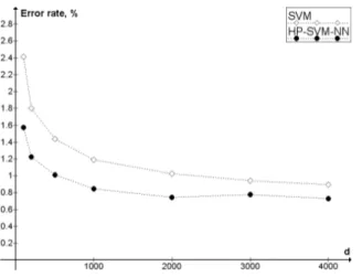
Figure 3: Comparison of SVM and HP-SVM-NN in terms of error rate. SVM is the pure SVM classifier, as imple-mented in SVMlight. HP-SVM-NN is the highest proba-bility SVM-NN classifier, as described in section 3.3. d is the number of features. C = 1.
speed such algorithm is not the same as N runs of basic SVM-NN classifier, because the costly operation of dis-tance calculation is performed only once for each classi-fied sample. Nevertheless, in this form the algorithm is very slow and needs some optimization to allow practical usage or fast experimental evaluation. The possibility for such optimization comes from the fact that with the small-est considered k for some samples all the nearsmall-est neigh-bors selected are from the same class. If such case occurs, it is considered sufficient evidence for taking the decision immediately and performing no future search. This ver-sion of the algorithm performs faster then the initial one, though obviously much slower that the pure SVM classi-fier nevertheless. The pseudocode of this optimized ver-sion of the algorithm is presented on the Figure 2.
4
Experimental Evaluation
4.1
Experimental Procedures
In order to evaluate the performance of the proposed al-gorithm and to compare it to the pure SVM classifier, we established two experiments, both of them using ten-fold
cross-validation on the SpamAssassin corpus1. The cor-pus contains 4150 legitimate messages and 1897 spam messages (spam rate is 31.37%). The partitioning of data is the same for all the runs. The linear kernel was used in both classifiers. The set of 25 possible values of the pa-rameter k ranges from 34 to 5334 with increasing steps. The following values of the number of features d were used: 100, 200, 500, 1000, 2000, 3000, 4000.
Feature extraction for SVM-based classification of email can be performed in different ways. In the exper-iment described below we used the following procedure. Each part of the message, namely the message body and each field of the message header, is considered as an un-ordered set of strings (tokens) separated by spaces. Pres-ence of a certain token in a certain part of a message is considered a binary feature of this message. Then, the d features with the highest information gain are selected. The information gain of a feature is defined as follows:
IG(fk) = X c∈{c1,c2} X f ∈{fk,¬fk} P (f, c) × log P (f, c) P (f ) × P (c) ,
where f is a binary feature, and c1 and c2 are the two classes of samples. Thus, each message is represented with a vector of d binary features.
The implementation of SVM used for this experiment is a popular set of open-source utilities called SVMlight2 [10]. Feature extraction is performed by a Perl script. The HP-SVM-NN classifier is implemented as a Perl script which uses SVMlight utilities as external modules for SVM training and classification.
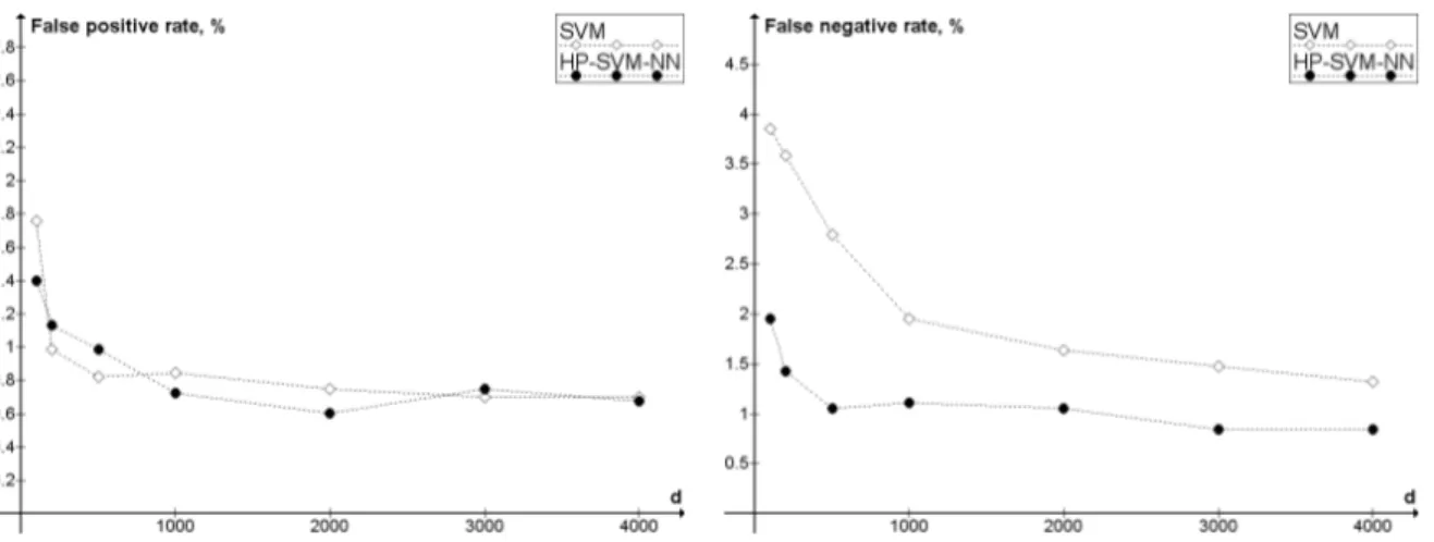
In the first experiment we compare the performance of the classifiers assuming that the error costs are equal. The parameter C is thus chosen equal to 1. The results of the comparison in terms of overall error rate are presented in Figure 3. The same results in terms of false positives (non-spam classified as spam) and false negatives (spam classified as non-spam) are given in Figure 4.
In the second experiment we compare the performance of the classifiers assuming that false positives are 9 times more expensive than false negatives. To adjust the relative
1Available at: http://spamassassin.apache.org/publiccorpus/ 2Available at: http://svmlight.joachims.org/
Figure 4: Comparison of SVM and HP-SVM-NN in terms of false positive rate and false negative rate. SVM is the pure SVM classifier, as implemented in SVMlight. HP-SVM-NN is the highest probability SVM-NN classifier, as described in section 3.3. d is the number of features. C = 1.
cost of errors for the HP-SVM-NN classifier, we select the parameter C = 19. For the SVM classifier we use the possibility of adjusting the relative error costs given by SVMlight. Weighted error rate is used instead of simple error rate in this case to judge the performance:
W Err9=
9 × nf p+ nf n np+ 9 × nn
where nf p is the number of false positives, nf n is the number of false negatives, np is the total number of positives (spam), and nnis the total number of negatives (non-spam). The results in terms of weighted error rate are given in the Figure 5. The same results in terms of false positives and false negatives are given in Figure 6.
4.2
Results
As we can see in Figure 3, the highest probability SVM nearest neighbor classifier achieves higher accuracy with all the considered values of d. The evaluation of sig-nificance of this advantage, performed using Wilcoxon signed-rank test with α = 0.05, showed that significance is present for all used values of d lower or equal to 2000, and not present for d = 3000 and d = 4000. The com-parison in terms of two types of errors (4) shows that the
Figure 5: Comparison of SVM and HP-SVM-NN in terms of weighted error rate. SVM is the pure SVM classifier, as implemented in SVMlight. HP-SVM-NN is the high-est probability SVM-NN classifier, as described in sec-tion 3.3. d is the number of features. False positives are considered 9 times more expensive than false negatives. C = 1/9.
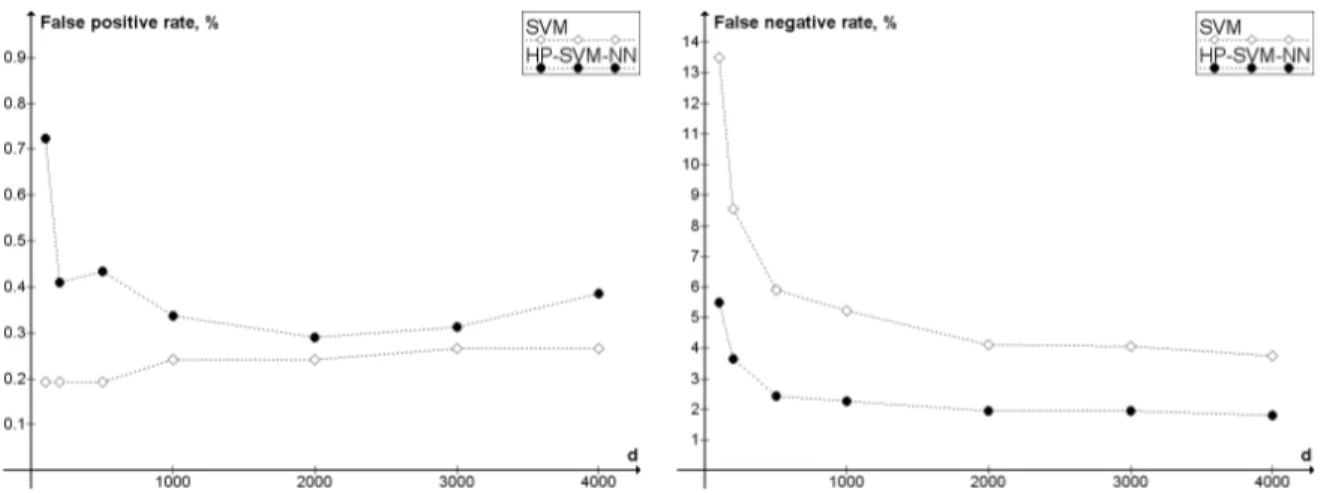
Figure 6: Comparison of SVM and HP-SVM-NN in terms of false positive rate and false negative rate. SVM is the pure SVM classifier, as implemented in SVMlight. HP-SVM-NN is the highest probability SVM-NN classifier, as described in section 3.3. d is the number of features. False positives are considered 9 times more expensive than false negatives. C = 1/9.
classifiers have close performance in terms of false pos-itives, but the HP-SVM-NN classifier is invariably better in term of false negatives.
However, in the case of unequal error costs, as it can be seen of Figure 5, none of the classifier achieves clear advantage. The result is slightly better for HP-SVM-NN with d = 1000, d = 2000 and d = 3000, but without being significantly different by means of Wilcoxon test.
Being more accurate that SVM, our classifier is at the same time obviously much slower. Our implementation, consisting of a Perl script and external modules that im-plement SVM, with the number of features d = 500 clas-sifier an optimized “easy” sample in about a second and a usual sample in about twenty seconds on a PC with CPU speed of 2.50GHz. It must be mentioned, however, that there is much space for optimization at the software level, by which serious, though not crucial, improvement on speed can be achieved. Also, it is possible to use a smaller set of possible values of k.
5
Conclusion
In this paper we proposed and discussed the highest prob-ability SVM nearest neighbor classifier. The classifier is a local SVM classifier, based on k samples in the
neigh-borhood of the sample to classify, k is selected dynam-ically among a pool of values depending on an estimate of the a-posteriori probability done following Platt [15]. Experimental comparison with the pure SVM classifier is performed, showing that our classifier is able to achieve better accuracy than SVM in the case of equal error costs. Thus locality proved to be a viable way of increasing the accuracy of the classification at the price of extra compu-tation. In the experiment with unequal error cost, how-ever, no significant difference is achieved, and further ex-perimental evaluation and improvement of the procedure of selecting the parameter k is needed.
References
[1] I. Androutsopoulos, G. Paliouras, V. Karkaletsis, G. Sakkis, C. Spyropoulos, and P. Stamatopoulos. Learning to filter spam e-mail: A comparison of a naive bayesian and a memory-based approach. In H. Zaragoza, P. Gallinari, and M. Rajman, editors, Proceedings of the Workshop on Machine Learning and Textual Information Access, 4th European Con-ference on Principles and Practice of Knowledge Discovery in Databases, PKDD 2000, pages 1–13, 2000.
[2] E. Blanzieri and A. Bryl. A survey of anti-spam techniques. Technical report #DIT-06-056. 2006. [3] E. Blanzieri and A. Bryl. Instance-based spam
filter-ing usfilter-ing SVM nearest neighbor classifier. In Pro-ceedings of FLAIRS 2007 (to be published), 2007. [4] E. Blanzieri and F. Melgani. An adaptive SVM
nearest neighbor classifier for remotely sensed im-agery. In Proceedings of 2006 IEEE International Geoscience And Remote Sensing Symposium, 2006. [5] C. Cortes and V. Vapnik. Support-vector networks.
Machine Learning, 20(3):273–297, 1995.
[6] N. Cristianini and J. Shawe-Taylor. Support Vector Machines. Cambridge University Press, 2000. [7] W. Cukier, S. Cody, and E. Nesselroth. Genres of
spam: Expectations and deceptions. In Proceedings of the 39th Annual Hawaii International Conference on System Sciences, HICSS ’06, volume 3, 2006. [8] H. Drucker, D. Wu, and V. Vapnik. Support vector
machines for spam categorization. IEEE Transac-tions on Neural networks, 10(5):1048–1054, 1999. [9] G. Hulten, A. Penta, G. Seshadrinathan, and
M. Mishra. Trends in spam products and methods. In Proceedings of the First Conference on Email and Anti-Spam, CEAS’2004, 2004.
[10] T. Joachims. Making large-Scale SVM Learning Practical. MIT-Press, 1999.
[11] C.-C. Lai and M.-C. Tsai. An empirical performance comparison of machine learning methods for spam e-mail categorization. Hybrid Intelligent Systems, pages 44–48, 2004.
[12] B. Leiba, J. Ossher, V. T. Rajan, R. Segal, and M. Wegman. SMTP path analysis. In Proceed-ings of Second Conference on Email and Anti-Spam, CEAS’2005, 2005.
[13] B. Medlock. An adaptive approach to spam filtering on a new corpus. In Proceedings of the Third Con-ference on Email and Anti-Spam, CEAS’2006, 2006.
[14] E. Moustakas, C. Ranganathan, and P. Duquenoy. Combating spam through legislation: A comparative analysis of us and european approaches. In Proceed-ings of Second Conference on Email and Anti-Spam, CEAS’2005, 2005.
[15] J. Platt. Probabilistic outputs for support vector machines and comparison to regularized likelihood methods. In A. Smola, P. Bartlett, B. Schoelkopf, and D. Schuurmans, editors, Advances in Large Margin Classiers, pages 61–74, 2000.
[16] M. Sahami, S. Dumais, D. Heckerman, and E. Horvitz. A bayesian approach to filtering junk e-mail. In Learning for Text Categorization: Papers from the 1998 Workshop. AAAI Technical Report WS-98-05, 1998.
[17] M. Siponen and C. Stucke. Effective anti-spam strategies in companies: An international study. In Proceedings of the 39th Annual Hawaii Interna-tional Conference on System Sciences, HICSS ’06, volume 6, 2006.
[18] L. Zhang and T. Yao. Filtering junk mail with a maximum entropy model. In Proceeding of 20th International Conference on Computer Processing of Oriental Languages, ICCPOL03, pages 446–453, 2003.
[19] L. Zhang, J. Zhu, and T. Yao. An evaluation of statistical spam filtering techniques. ACM Trans-actions on Asian Language Information Processing (TALIP), 3(4):243–269, 2004.