Development and Verification of Calculation Models for the Accident Analysis in Nuclear Power Plants

(1)

Developrnent and Verification of Calculation Models for the Accident Analysis in Nuclear Power Plants.

Descrittori

Tipologia del documento: Rapporto Tecnico

Collocazione contrattuale: Accordo di programma ENEA-MSE: Piano Annuale di

Realizzazione 2013, Linea Progettuale 1,Obiettivo A: Acquisizione,

Sviluppo eValidazione di Codici e Metodi per Studi ed Analisi di Sicurezza eSostenibilità, Task A3.1&2.

Argomenti trattati: Sicurezza Nucleare Sommario

This report presents the activities perfo.rmed in the frame of LPl, Objective A (Acquisition,

development and validation of methods and codes for sustainable and safety studies and analyses),

Task A3.1&2 of PAR2013, ADP ENEA-MSE. New plenurn temperature models are under development to refi ne the accuracy of the TRANSURANUS code under steady-state and accident conditions (LOCA, RlA). For the purpose, a 2D transient heat transfer model and a finite elements model have been developed. In this frame, ENEA has introduced in TRANSURANUS the FRAPCON-3 plenum temperature model. Furthermore, pre-test analysis of debris bed reflooding experiments have been performed with the ICARE/CA THARE code to support the PEARL experimental program at IRSN and verify the capability of the new 2D porous media model

implemented in the last version of the code. Moreover, the calculation of degraded core reflooding scenarios has been performed with the ASTEC code in the frame of the TMI-2 Benchrnark Exercise

promoted by the OECD. Besides the important achievements in code model development,

improvement and verification, these activities contributed to strengthen research collaborations with foreign partners at intemational level and acquire tools and their knowledge for safety analysis aoolications to the existinz nuclear oower olants located near the border of our countrv.

Note:

Authors:

G. Bandini, R. Calabrese, S. Ederli (ENEA)

FIRMA NOME 2 FIRMA NOME 1 FIRMA

o

EMISSIONE 17/09/14 t--_N_OM_E_~:-G_. B_an_d_tin--1_---7i itt?,..'~'h-le--l~f-c0""1'lsr-a-+----#~"f:-P_ce,Rr-0#)~_:a--l

~

l

--=-

A

--

Vi

!hJk

M

(;JjlJ

&L

'

"

REDAZIONE \l CONVALIDA IlAPPROVAZIONE

(2)

List of Contents

1. Introduction ……….…. 3

2. Upper plenum temperature calculations: comparison of TRANSURANUS with a 2D model under steady-state conditions ………..………..….… 4

2.1 TRANSURANUS models for plenum temperature ... 4

2.1.1 Standard version options ………..….. 4

2.1.2 2D transient model ……….………..…… 4

2.1.3 FRAPCON-3 model ……….… 5

2.2 COMSOL 2D model ………….……….…. 7

2.3 Comparisons of models ………..……… 8

2.4 Results and discussions ……….. 9

2.5 Final remarks ………..… 11

3. Complementary ICARE/CATHARE calculations to support the experimental program PEARL ………... 13

3.1 Brief description of the PEARL facility ……….…… 13

3.2 ICARE/CATHARE modeling of the PEARL facility ……….... 14

3.2.1 Minor modifications to account for the new radial size of heated debris bed and bypass ……….………...…. 14

3.2.2 Experimental scenario and boundary conditions ………..…… 15

3.3 ICARE/CATHARE numerical results ……….…….….. 16

3.3.1 Heat-up and filling phase ………..…. 16

3.3.2 Reflooding phase ………..… 17

3.3.2.1 Water flow rate equal to 5 m/h ……….……..…. 17

3.3.2.2 Water flow rate equal to 10 m/h ………..… 19

3.3.2.3 Water flow rate equal to 15 m/h ………..…… 20

3.3.2.4 Water flow rate equal to 30 m/h ………..… 21

3.4 Final remarks ………. 22

4. Calculation of degraded core reflooding scenarios in the TMI-2 plant with the ASTEC code ………..… 48

4.1 Description of code models used ……… 48

4.2 TMI-2 plant and core nodalization ……….…….…... 49

4.3 TMI-2 plant initial conditions ……….... 50

4.4 SLB sequence and reflooding scenarios ………...….…….…... 52

4.5 Analysis of results ……….……….….…... 52

4.6 Final remarks ………...……….……...…... 62

(3)

1. Introduction

The in-depth analysis of design basis and severe accidents in existing and future nuclear power plants requires the use of qualified numerical tools provided with models able to simulate in a consistent and reliable way all different phenomena that might occur during the various phases of an accident, starting from its initiating event up to the eventual release of radioactive materials into the environment. Furthermore these models shall be able to assess the effectiveness of accident management measures which might be taken to mitigate the consequences of these accidents.

This report present the results of the activities performed by ENEA in the frame of Tasks 3.1 & 3.2 of PAR2013 – LP1 and devoted to the development and verification of code models used in the analysis of accidents in nuclear power plants. The report is structured in three different sections dealing with:

 Section 21_{- New plenum temperature models are under development to refine the}

accuracy of the TRANSURANUS code under steady-state and accident conditions (LOCA, RIA). Efforts have been undertaken to improve the description of the plenum volume sub-system by means of 2D models. For the purpose, a 2D transient heat transfer model and, besides this, a finite elements model, implemented by means of the commercial software COMSOL Multiphysics, have been developed. For comparison, ENEA has introduced in TRANSURANUS the FRAPCON–3 plenum temperature model as well. This section presents the models and their predictions for a PWR fuel pin under steady-state conditions. In addition, preliminary results on the effect of fission gas release are discussed.

 Section 3 – Complementary pre-test analyses of PEARL debris bed reflooding experiments with the ICARE/CATHARE code in the frame of the bilateral cooperation between ENEA and IRSN. The main aim of this work is to support IRSN in the definition of geometry and boundary conditions of the tests that will be carried out in the PEARL facility, and at the same time verify the capability and consistency of the improved porous media models recently implemented in the last version of the code.  Section 4 - The analysis of degraded core reflooding scenarios with the European

ASTEC code, during an alternative severe accident sequence (SBLOCA) simulated on the TMI-2 plant, in the frame of ENEA participation in the activities of the Benchmark Exercise promoted by the OECD/NEA/CSNI. The main aim of this work is to verify the robustness of the code under the most severe accident conditions and assess degraded core coolability by late intervention of emergency core cooling systems.

Finally, the main achievements and conclusions of the above mentioned ENEA activities are summarized in Section 5.

1_{The content of this section was presented at the 23}rd_{International Conference “Nuclear Energy for New Europe”,}

September 8−11, 2014, Portorož, Slovenia, paper 918. Authors: R. Calabrese (ENEA), A. Schubert (JRC-ITU), P. Van Uffelen (JRC-ITU), L. Vlahovic (JRC-ITU), Cs. Győri (NucleoCon).

(4)

2. Upper plenum temperature calculations: comparison of

TRANSURANUS with a 2D model under steady-state condition

The fuel rod inner pressure is calculated through the definition of the temperature of each free volume filled with gas (upper plenum, lower plenum, gap, cracks, etc.) [1]. In LWR fuel rods a fraction between 40 and 50% of the filling gas is located in the upper plenum. Moreover, the rod internal gas pressure increases under irradiation due to the accumulation of gaseous fission products released into the free volume. To offset the increasing number of moles of fission gas, a reduction of the heat rate is applied towards the end of irradiation in the higher power cases [2]. Therefore, the accurate computation of the plenum temperature is an important issue for the assessment of fuel safety.

The TRANSURANUS modelling is under development to improve the description of the upper plenum temperature under steady-state and accident conditions. The report presents the models under consideration (2D transient, 2D COMSOL Multiphysics, FRAPCON–3) and a comparison of their predictions for a typical 17x17 PWR fuel rod under steady-state conditions [2]. The paper focuses on the contribution of conductive, convective and gamma heating to the heat transfer occurring between the plenum volume and coolant. In the concluding part, preliminary calculations on the effect of fission gas release on the plenum temperature are presented.

2.1 TRANSURANUS models for plenum temperature 2.1.1 Standard version options

For the calculation of the average temperature in the upper plenum, the TRANSURANUS code offers a "low” temperature and a “high” temperature model [1]. In the first, the plenum temperature is coincident with the coolant temperature at the uppermost section, in the second, the temperature is calculated by means of a weighted sum of the cladding inner temperature and the fuel central temperature referring, as previously, to the uppermost slice.

2.1.2 2D transient model

The new 2D transient model implemented in the TRANSURANUS code considers the plenum gas in a static condition under the hypothesis that the convective and the radiative heat transfers are negligible in comparison with the conductive contribution. The model calculates the heat conduction in the plenum volumes means of a finite volume approach in a two dimensional geometry (r, z). According to the time constants of the plenum gas (1–5 s) and cladding (~0.05 s), the model adopts a transient analysis approach for the first and a quasi-stationary for the second.

Some relevant characteristics of the model are briefly resumed: ─ system of linear equations;

(5)

─ optional solution schemes; ─ standard mathematical routines.

The heat transfer process is described by means of an integral form of the Fourier equation for the 2D (r, z) domain Ω:

           d d z r r r a d d k k ij k k ij

 

                                       1 1 2 2 2 2 1 (1)

Crank–Nicolson, Forward Euler (explicit) and Backward Euler (implicit) schemes are the three optional methods developed for the solution of Eq. (1). The use of CPU time resources depends on the number of nodes used for the geometric description of the plenum volume. Time step controls assure the numerical stability and convergence of the solution.

2.1.3 FRAPCON−3 model

The model predicts the plenum temperature by means of three terms: the energy transfer between the top of the fuel stack and the plenum gas, between the plenum gas and the coolant channel and, finally, between the plenum spring, heated by gammas, and coolant [3]. The model is applicable under steady-state conditions. The convective term is an empirical correlation for the heat transfer between horizontal plates [4]:

D kNu

h_p  (2)

where:

hp heat transfer coefficient (W / m2 K);

Nu Nusselt number (–);

k thermal conductivity of the plenum gas (W / m K);

D cladding inner diameter – hot condition (m).

The value of the Nusselt number, calculated through the following correlation, is strongly dependent on the regime of heat transfer. A laminar regime is assumed for values of the Rayleigh number up to 2·107, thereafter a turbulent regime is fully developed [3]. In the Eq. (3), the values assumed for the coefficients C and m are 0.54, 0.25 and 0.14, 1/3 in laminar and turbulent regime, respectively.

m Gr C Nu ( Pr) (3) where: Gr Grashof number (–): Pr Prandtl number (–).

(6)

The second term of the FRAPCON–3 model deals with the calculation of the conductive heat transfer between the plenum gas and coolant according to the correlation (4) [3]. DB o clad i o f c h T D K D D Dh U ) 0 . 1 ( 0 . 2 ln 0 . 2 0 . 1             (4) where:

Uc plenum-to-coolant effective conductivity (W / m K);

hf heat transfer coefficient at the cladding inner surface (W / m2 K);

kclad cladding thermal conductivity (W / m K);

D cladding inner diameter – hot condition (m);

hDB heat transfer coefficient at the cladding outer surface (W / m2 K);

Di, Do cladding inner and outer diameter – cold condition (m);

α cladding thermal expansion coefficient (1 / K).

This correlation has been implemented in TRANSURANUS by assuming that the laminar layer between the plenum spring and cladding is equal to the initial gap width. In the presented calculations, this value is kept constant. The heat transfer coefficient at the cladding inner surface has been modelled according to the URGAP subroutine [1]. The cladding-to-coolant heat transfer coefficient was defined according to the evaluations of TRANSURANUS (ALPHAL) in the uppermost slice [1].

The third term of the plenum temperature model accounts for the spring gamma heating [3]. This contribution is calculated by means of correlation (5) under the hypothesis that the gamma component is 10% of the power flux and that the attenuation coefficient in the plenum spring is 37.6 (1/m). The average heat flux was calculated accounting for the total inner surface of the cladding under the hypothesis that the radiative source is isotropic.

spring

irr QV

Q 3.76 (5)

where:

Qirr spring gamma heating (W);

Q rod average heat flux (W / m2);

Vspring spring volume (m3).

(7)

4 4 2 2 2 2 D h D V U D h T T D V U Q T p p c p pa BLK p c irr plenum       (6) where:

TBLK bulk coolant temperature (K);

Tpa fuel average temperature in the uppermost slice (K);

D cladding inner diameter – hot condition (m);

Vp plenum volume (m3).

The plenum temperature model introduced in the code accounts for a filling gas mixture composed of helium, xenon, and krypton. For the purpose, the URGAP correlations for the thermal conductivity (IHGAP=3) and dynamic viscosity have been employed [1]. The calculation of density and specific heat was based on values found in the open literature [5]. The description of the thermophysical properties dependence on temperature and pressure needs further improvements.

2.2 COMSOL 2D model

The models presented in the previous sections have been introduced as part of the TRANSURANUS source code whereas the COMSOL Multiphysics model was developed as a stand-alone application [6]. The heat transfer process in the geometric domains under consideration (fuel, cladding, spring, plenum gas) is described by means of Eq. (7).



k T



Q ρC T t T ρC_P      _P    u (7)

In this equation, T stands for temperature, Q for the volumetric heat source (only for the fuel and spring). The thermophysical properties , CP and k are, the density, specific heat

and thermal conductivity of each domain under consideration.

In this model, the radiative contribution to the heat transfer was neglected. The effect of convection is embedded in the second term in the right part of the eq. (7) where u is the velocity vector. This term is included only in the model for the upper plenum2. The velocity field of helium in the upper plenum is calculated according to the Navier-Stokes equations (8a, 8b) for a laminar flow regime.

(8)

g u u u p t u ρ u t T                       _ __ _ __               3 2 0 (8a, 8b)

In the Eq. 8a and 8b, p stands for the pressure of fluid and I for the identity matrix,  is the fluid dynamic viscosity and gthe gravity acceleration. The equations express the conservation of mass (8a) and momentum (8b). The rightmost term in the second equation accounts for the effect of buoyancy that is basically natural convection. For solving the given equations, the following boundary conditions need to be defined: cladding outer temperature, volumetric heat source within the fuel, gamma heating of the spring.

In order to avoid discontinuities in the cladding temperature, the axial power profile was interpolated by means of a smoothing function in such a way that it drops to zero at a level of 40 mm above the top of the fuel stack (Figure 2.1).

Figure 2.1: Smoothing function at the border fuel stack / plenum

2.3 Comparisons of models

The comparison of presented models was performed under conditions typical for a 17x17 PWR fuel rod as resumed in Figure 2.2 [2]. At the top of the fuel stack, the linear heat rate was about 60% of the peak value (22.97 kW/m) [2]. In the COMSOL calculations, a constant radial power profile and a cosine-shaped axial power profile were assumed whereas the cladding outer temperature boundary condition was defined by means of a simplified thermal-hydraulic model. The determination of the spring gamma heating relied on the correlation (5) [3]. The values of the fuel average temperature and coolant temperature applied in the TRANSURANUS analysis were set in agreement with the values adopted in the COMSOL analysis. The geometrical model employed in the comparison consists of the upper part of the fuel stack (0.05 m) and the plenum volume as shown in Figure 2.2. This analysis

Serie2; 3.61; 13.8723753 9 Serie2; 3.615; 13.8723745 3 Serie2; 3.62; 13.8723715 Serie2; 3.625; 13.8723609 3 Serie2; 3.63; 13.8723240 5 Serie2; 3.635; 13.8721953 Serie2; 3.64; 13.8717459 7 Serie2; 3.645; 13.8701778 6 Serie2; 3.65; 13.8647073 9 Serie2; 3.655; 13.8456473 6 Serie2; 3.66; 13.77953 Serie2; 3.665; 13.5536250 3 Serie2; 3.67; 12.8200425 7 Serie2; 3.675; 10.7829957 4 Serie2; 3.68; 6.93618787 1 Serie2; 3.685; 3.08938000 4 Serie2; 3.69; 1.05233317 6 Serie2; 3.695; 0.31875070 9 Serie2; 3.7; 0.09284574 3 Serie2; 3.705; 0.02672838 7 Serie2; 3.71; 0.00766835 3 Serie2; 3.715; 0.00219788 7 Serie2; 3.72; 0.00062977 6 Serie2; 3.725; 0.00018044 Serie2; 3.73; 5.16973E-05 Serie2; 3.735; 1.48116E-05 Serie2; 3.74; 4.24359E-06 Serie2; 3.745; 1.21581E-06 Serie2; 3.75; 3.48335E-07 Serie2; 3.755; 9.97997E-08 Serie2; 3.76; 2.85931E-08 Linear Power kW/m z / m

(9)

deals with a very short irradiation history (120 s) during which the COMSOL model defines the absolute value of the inner pressure and reaches the steady state. Due to the Navier-Stokes equations, the model is not stable by solving a stationary problem.

Reference design data [2]

Pitch (mm) 12.6

Cladding OD (mm) 9.4

Cladding thickness (mm) 0.61

Gap thickness (mm) 0.084

Fuel pellet and spring diameter 8.0

Pellet length (mm) 11.4

Plenum length (mm) 254

Turns in the plenum spring 28

Plenum spring wire diameter (mm) 1.27

Helium fill gas pressure (MPa) 2.41

Active fuel length (m) 3.66

System pressure (MPa) 15.5

Coolant inlet temperature (°C) 277

Coolant flow rate (106kg/m2h) 12.47

Pellet density (%TD) 95

Figure 2.2: Fuel rod specifications and fuel section modelling (rodlet approach)

2.4 Results and discussion

The models’ results are presented in Table 2.1. The table resumes the values of the upper plenum temperature and pressure at the end of transient (120 s).

Table 2.1: Results at the end of the short irradiation history (120 s) – upper plenum

TRANSURANUS models COMSOL model "low" temperature "high" temperature 2D transient FRAPCON−3 Temperature (K) 598.37 720.75 601.25 600.16 600.94 Pressure (MPa) 4.83 5.81 4.86 4.85 4.84

The results confirm that the models are in fair agreement with small deviations from the code “low” temperature option. The values of the 2D transient model presented in Table 2.1 refer to the Crank–Nicolson solution scheme whereas the results of the solution algorithms are gathered in Figure 2.3.

In these preliminary simulations, no fission gas release occurs and the presented results refer to a helium-filled plenum. The agreement shown in the models’ predictions is understandable when considering that the conductive heat transfer is the dominant

(10)

contribution. This hypothesis is confirmed by the low value of the Rayleigh number calculated by the FRAPCON–3 model fully consistent with a laminar regime of the convective heat transfer that is well described in the COMSOL model. In general, the contribution of the gamma heating is of minor importance.

Figure 2.3: Plenum temperature: 2D transient model (left side), COMSOL (right side) A further calculation was performed by means of TRANSURANUS on an integral fuel rod consistent with the data resumed in Figure 2.2. In this analysis, the irradiation reaches a burn-up of about 56 GWd/t at constant heat rate consistent with the values presented in Section 2.3. The results of this analysis are shown in Table 2.2.

Table 2.2: Results at the end of the irradiation history (56 GWd/t) – upper plenum Models "low" temperature "high" temperature FRAPCON−3

Temperature (K) 594.73 746.29 603.27

Pressure (MPa) 8.17 9.90 8.27

The FRAPCON–3 model introduced in TRANSURANUS treats the presence of the xenon and krypton fission products vented to the free volume of the fuel rod. The results presented in Table 2.2 deal with a fission gas release of 3.86% at the end of irradiation. The values of the upper plenum pressure are higher than the corresponding results presented in Table 2.1 accounting for the presence of free volumes at higher temperatures not taken into account in the simplified geometry adopted in the previous analysis. Moreover, the increase seen in the prediction of the "high" temperature model confirms the effect of fission gas

595 597 599 601 603 605 0 40 80 120 Forward Euler Crank-Nicolson Backward Euler Time (s) Pl enum T e m peratur e (K)

(11)

release on the average fuel temperature of the uppermost fuel section. This consideration is confirmed in the results of the FRAPCON–3 model where the deviation of the upper plenum temperature if compared to the results of the ”low” temperature option is higher than in Table 2.1. The Rayleigh number moves from a value of 0.37·105 at the beginning of irradiation to a value of 0.54·107_{at the end of irradiation thus approaching the transition to a turbulent regime}

[3]. Across the irradiation, the Prandtl number moves from 0.68 to 1.16 and the Grashof number from 0.55·105 to 0.48·107.

Two factors may affect the regime of convection: the increase of the fuel central temperature due to the degradation of the gap conductance and the change in the thermophysical properties of the gas mixture. The density of the gaseous fission products xenon and krypton is notably higher than helium [5]. According to the COMSOL results in the rodlet geometry, TRANSURANUS is expected to overestimate the first factor not accounting for the effect due to the presence of the plenum spring. As shown above, the value of the Prandtl number is slightly changing with the composition of the gas mixture. On the contrary, the value of the Grashof number has a significant dependence on the filling gas composition. With a plenum temperature of 600 K and values of the inner pressure ranging in the interval 2–8 MPa, the Grashof number increases, for a common geometry and ΔT, by a factor 550–600 if, instead of helium, xenon is adopted as filling gas [5]. According to these observations, the values of the Rayleigh number calculated for a rodlet filled with helium was 0.23·105 while for a xenon-filled rodlet this value increases to 0.40·108 well beyond the onset of a turbulent regime for the convective term. For a xenon-filled rodlet, the FRAPCON–3 model predicted a plenum temperature higher than presented in Table 2.1 (633.52 K) while no significant deviations were noted in the results of the 2D transient model (599.14 K).

2.5 Final remarks

A comparison of the models developed to refine the TRANSURANUS evaluations of the upper plenum temperature has been presented. The models’ predictions showed a good agreement under the conditions selected for the comparison and indicated that the conductive heat transfer has a prominent role in helium rods. The results of the FRAPCON–3 model showed that fission gas release could cause a transition from a laminar to a turbulent regime of heat transfer. Therefore, the hypothesis of negligible convective contribution to heat transfer assumed in the 2D models should be reconsidered in the case of significant fission gas release. A limited effect was noted for the gamma heating of the plenum spring. These preliminary conclusions will be further assessed and verified. Geometrical effects not modelled in a 1.5 dimensional code and transient conditions will be considered as well.

References

1. K. Lassmann, “TRANSURANUS: a fuel rod analysis code ready for use”, Journal of

(12)

2. G. M. O'Donnell, H.H. Scott, R. O. Meyer, "A New Comparative Analysis of LWR Fuel Designs", Technical Report, NUREG-1754, U.S. Nuclear Regulatory Commission (2001).

3. G. A. Berna, C. E. Beyer, K. L. Davis, D. D. Lanning, "FRAPCON-3: A Computer Code for the Calculation of Steady-State, Thermal-Mechanical Behavior of Oxide Fuel Rods for High Burnup", Technical Report, NUREG/CR-6534 (vol. 1 & 2), U.S. Nuclear Regulatory Commission (1997).

4. H. W. McAdams, "Heat transmission", McGraw-Hill Series in Chemical Engineering (1954).

5. J.-M. P. Tournier, M. S. El-Genk, "Properties of noble gases and binary mixtures for closed Brayton Cycle applications", Energy Conversion and Management 49, 469–492 (2008).

(13)

3. Complementary ICARE/CATHARE calculations to support the

experimental program PEARL

The experimental program PEARL has been designed by IRSN to study the reflooding process of a debris bed, considering higher temperatures and higher pressures with respect to experiments carried out in the past. Moreover, the diameter of the test section is large enough to allow 2D/3D effects in the water penetration through the debris bed.

The debris bed is composed of stainless steel spheres heated by induction and enclosed by an unheated debris bed composed of quartz spheres and called bypass.

In the frame of the bilateral cooperation with IRSN, the ENEA has already completed a series of ICARE/CATHARE pre-test calculations to support the IRSN in the definition of geometry and boundary conditions of the tests that will be carried out in the PEARL facility [1].

The main result of the performed studies was those 2D effects, consisting in the preferential water progression through the unheated debris bed outer region (bypass), mainly depends on the assumed water flow rate. Increasing water flow rate and steam production rate, the pressure gradient between the debris bed center and the periphery also increases, favoring the water flow through the bypass to the detriment of the inner region of the heated debris bed. 2D effects becomes not negligible only when the water velocity in the debris bed (40% of porosity) is higher than 15 m/h.

The features of the bypass region, as particles size and porosity, have conversely a negligible effect on the reflooding behavior and the water flow rate, after which 2D effects take place, is basically independent by the features of the bypass.

The objective of the present work is to investigate the effect of the bypass thickness on the reflooding behavior. In particular we want to study if a ticker bypass region can promotes the onset of 2D effects at a lower water flow rate. For this purpose the calculations performed with different water flow rates have been repeated, assuming a larger unheated outer region to the detriment of the heated debris bed.

3.1 Brief description of the PEARL facility

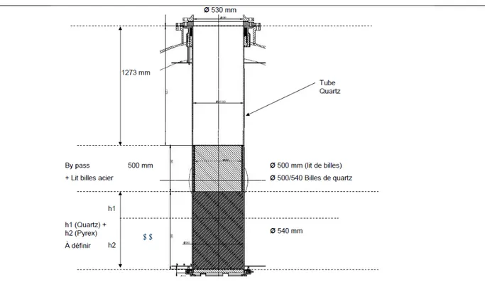
The plan of the PEARL facility is represented in the Figure3.1. The inlet circuit enables the injection of steam and/or water at the bottom of the test section. The outlet circuit, at the top of the test section, allows to collect water and condensed steam in a container of 250 liters. Different values of pressure can be imposed. The test section is set in a nitrogen atmosphere, maintained at a constant temperature of 200°C (473 K).

The provisional plan of the test section is reported in the Figure 3.2. A quartz cylindrical duct, which inner diameter is 540 mm, contains the debris bed composed of stainless steel spheres. Induction heating is used to generate power within the debris bed.

(14)

The stainless steel debris bed has a diameter of 500 mm and it is separated from the quartz tube by an unheated debris bed composed of quartz spheres. Such outer region, called bypass, has a thickness of 20 mm and should have higher porosity and permeability than the heated stainless steel debris bed.

The above described debris bed size is the one considered in the previous ICARE/CATHARE pre-test calculations. The new calculations will be based on a bypass thickness of 32.83 mm that increases the cross section of the bypass of about 60%. The external diameter of the heated debris bed becomes then 474.34 mm that reduces the cross section of about 10%.

The stainless steel debris bed and the bypass are supported by a double layer of unheated debris bed; the lowest one composed by pyrex spheres and the above one by quartz spheres.

3.2 ICARE/CATHARE modeling of the PEARL facility

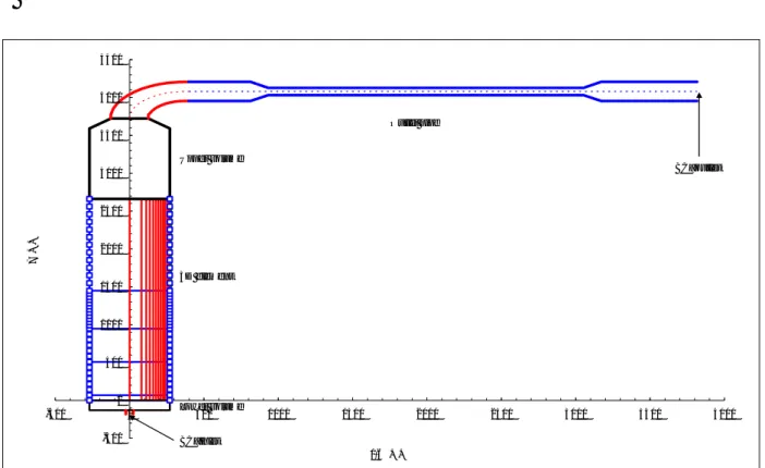
The ICARE/CATHARE modeling of the PEARL facility is basically the same of the previous calculations and it is represented in Figure 3.3. The solid structures of the test section, including the quartz tube and debris beds, are represented with ICARE2 2D axial symmetric components. The ICARE2 2D element extends axially from 0 to 2.66 m.

CATHARE2 volume elements (0D geometry) roughly simulate the void volumes of the PEARL facility below and above the ICARE2 2D element. Inlet and outlet pipelines are represented by CATHARE2 pipe elements (1D geometry). The water-steam behavior within volume and pipe elements is calculated with standard CATHARE2 model. A specific 2D model, adapted for porous medium characteristics, is adopted within the debris bed.

Boundary conditions are imposed at the inlet (steam-water flow rate and temperature) and outlet (pressure) pipes.

3.2.1 Minor modifications to account for the new radial size of heated debris bed and bypass

The different debris bed regions which their main features are illustrated in Figure 3.4. The only modification of the previous modelling concerns the radial size of the heated debris bed and bypass. Pyrex and quartz debris bed remain unchanged. The main features of the heated debris bed and bypass are detailed in Table 3.1.

(15)

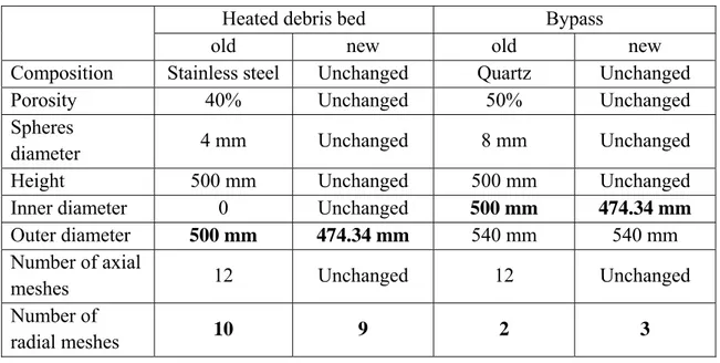
Table 3.1: Heated debris bed and bypass main features

Heated debris bed Bypass

old new old new

Composition Stainless steel Unchanged Quartz Unchanged

Porosity 40% Unchanged 50% Unchanged

Spheres

diameter 4 mm Unchanged 8 mm Unchanged

Height 500 mm Unchanged 500 mm Unchanged

Inner diameter 0 Unchanged 500 mm 474.34 mm

Outer diameter 500 mm 474.34 mm 540 mm 540 mm

Number of axial

meshes 12 Unchanged 12 Unchanged

Number of

radial meshes 10 9 2 3

Differences between new and old debris bed dimensions are underlined. The number of axial and radial meshes adopted in the numerical simulation is also indicated.

The whole radial meshing (heated debris bed plus bypass) is not changed and the new bypass simply includes an additional radial mesh that was the outermost radial mesh of the old heated debris bed. The same radial meshing has been adopted to simplify the comparison between old and new numerical results.

3.2.2 Experimental scenario and boundary conditions

The experimental scenario and boundary conditions are the same of the previous calculations. They are reported hereafter. The pressure is imposed as outlet boundary condition and set to 3 bar during the whole simulated transient.

The preliminary heat-up phase, designed to reach a maximum debris bed temperature of 1073 K (700°C), is characterized by the injection of overheated steam at 473 K (200°C), at very low flow rate (0.4201·10-3_{kg/s), during 1900 s. The specific power of the heated debris bed is}

the same of the previous calculations (127.7 W/kg). The total power is clearly reduced of about 10%, as the cross section of the heated debris bed.

At 1900 s, the steam injection is stopped and a very high water flow rate is imposed (2.9646 kg/s), until 1940 s, to fill the bottom part of the test section, including pyrex and quartz non heated debris beds.

At 1940 s, when the water level is roughly at the bottom of the heated debris bed (948 mm of axial level), the water flow rate is set to the targeted one for the reflooding phase. The calculations performed with different reflooding flow rates will be then repeated taking into account the new heated debris bed and bypass radial size.

(16)

The injected water temperature, during filling and reflooding phases, is 381.54 K (108.54°C), corresponding to 25°C of subcooling.

At the beginning of the heated debris bed reflooding (1940 s), the specific power is also increased from 127.7 W/kg to 150 W/kg. Also in this case the total power is 10% lower than the one of the previous calculations.

3.3 ICARE/CATHARE numerical results

Four calculations have been carried-out, with the new ICARE/CATHARE modelling (thicker bypass), imposing different injected water flow rates during the reflooding phase: 5, 10, 15 and 30 m/h. The given water flow rates are expressed as equivalent water velocities in a debris bed 40% of porosities that radially extends on the whole PEARL test section.

In order to make a proper comparison between the obtained numerical results, the selected water flow rates are the same investigated in the previous calculations, except for 40 m/h of water flow rate, not considered in the new calculations. The new calculations will be identified as “Large bypass” and the previous ones as “Regular bypass”.

3.3.1 Heat-up and filling phase

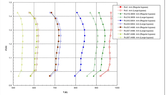
The heat-up (0-1900 s) and filling (1900-1940 s) phases are common to all calculations. The heated debris bed and bypass temperatures at the end of the overheated steam phase (1900 s) are presented in Figure 3.5, in the form of axial profiles at different radial locations.

The bypass thickness has a negligible effect on the central temperature of the heated debris bed (R = 0 mm) that is basically the same in both calculations and it is very close to the targeted one (973 K).

The radial gradient of temperature is on the contrary clearly affected by the bypass size and the temperature of the outer mesh of the bypass (R = 267.4486 mm) predicted by the “Large bypass” calculation is 60 - 70°C lower than what observed in the “Regular bypass” case.

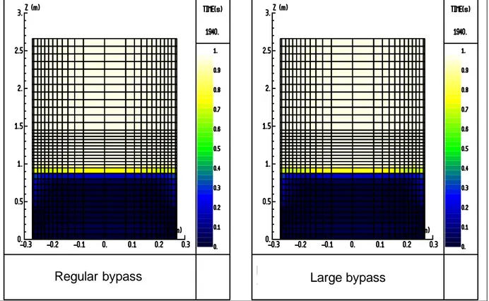
The temperature distribution in the different debris bed regions and in the cylindrical wall of PEARL test section, predicted by “Regular” and “Large bypass” calculations at the end of the filling phase (1940 s), is illustrated in Figure 3.6.

The temperatures of the pyrex and quartz debris bed, from 0.068 to 0.948 m of axial level, are very close to the injected water temperature (381.54 K).

A large portion of the heated debris, from 0.948 to 1.448 m, is characterized by nearly uniform temperature. Sudden temperature decreases can be observed in the vicinity of the underlying quartz debris bed (axial direction) and, in radial direction, near the boundary between the stainless steel debris bed and the bypass.

(17)

In the case of “Large bypass” configuration, the radial extent of the region at uniform temperature is lower than what observed in the “Regular bypass” calculation. Symmetrically, the radial extension of the external colder region is greater in the “Large bypass” calculation whit respect to what predicted in the “Regular bypass” case.

The effect of assumed bypass size on the void fraction distribution at the end of the filling phase (Figure 3.7) is negligible. One can observe that the water level is, in both calculations, very close to the bottom of heated debris bed and bypass (axial level = 0.948 m).

3.3.2 Reflooding phase

The results of the new calculations (“Large bypass”), obtained with different flow rates during the reflooding phase, are described in the next paragraphs and compared to the ones of the previous calculations (“Regular bypass”).

3.3.2.1 Water flow rate equal to 5 m/h

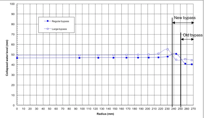
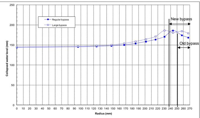
The Figure 3.8 shows the radial profile of the collapsed water level, measured from the bottom of heated debris bed and bypass, at the beginning of the reflooding phase (1970 s). One can observe that in both “Regular” and “Large bypass” calculations, the collapsed water level in the bypass is lower than in the heated debris bed and it exhibits a peak at the boundaries between the stainless steel debris bed and the bypass. This is due to capillary pressure difference between the bypass (greater particles diameter and porosity) and the heated debris bed that removes some water from the bypass toward the outer side of the heated debris bed.

In the “Large bypass” calculation, the observed peak is shifted inwards, that is consistent with the larger size of the bypass. Except for this, the differences with the “Regular bypass” case are minimal.

The debris bed behavior during the reflooding is well illustrated from Figure 3.9 to Figure 3.17 that show, for both “Regular” and “Large bypass” cases, the temperatures distribution in the debris bed, the void fraction and the radial profile of the collapsed water level at 2100 s, 2300 s and 2600 s of transient time.

The temperature distribution in the debris bed puts into evidence the effect of the bypass size on the radial extension of the “cold” region at the debris bed edge: slightly greater in the “Large bypass” case. The differences between the two calculations gradually decrease during the course of the transient and, at 2600 s (Figure 3.11), the temperature distribution provided by two calculations is very similar.

The void fraction distribution (Figure 3.12 to Figure 3.14) is practically independent on the bypass size and, in both calculations, the swollen water level remain almost flat indicating a quasi 1D water progression through the debris bed.

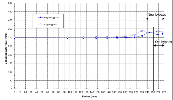
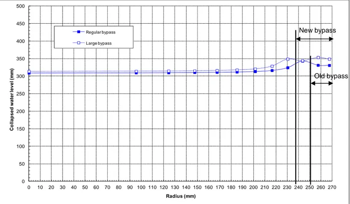
The collapsed water level (Figure 3.15 to Figure 3.17) is in general slightly higher in the “Large bypass” case, indicating a little greater axial progression velocity of the water

(18)

front. This is probably linked with the steam production rate that, due to the lower debris bed average temperature and power (10% less), is slightly lower with respect to the “Regular bypass” calculation. The differences are, however, very limited and tend to decrease during the course of the transient.

In both calculations, the collapsed water level at 2100 s (Figure 3.15) is slightly lower in the bypass than in the heated debris bed. As before mentioned, this is due to the capillary pressure that removes some water from the bypass toward the outer side of the heated debris bed. With the gradual increase of the water level during the course of the transient, the effect of capillary pressure is contrasted by gravity and friction forces and the collapsed water level becomes flatter and even slightly higher in the bypass than in the central region of the heated debris bed (Figure 3.16 and Figure 3.17). The described behavior can be observed in both calculations.

In any case the radial profile of the collapsed water level doesn’t show any significant preferential penetration of the water through the bypass and the increase of the bypass size is not able to induce 2D effects at the considered water flow rate.

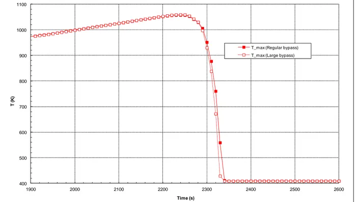
The Figure 3.18 shows the evolution vs. time of the maximum debris bed temperature. The results of “Large” and “Regular bypass” calculations are plotted in the same figure.

One can remark that the quenching of the whole debris bed is slightly anticipated in the case of “Large bypass” calculation. This is consistent with the axial progression of the water that, as before explained, is a little faster than in the case of “Regular bypass”.

The evolution vs. time of temperature and void fraction in the outer side of the bypass (radial mesh 12), at the top (last axial mesh) of the debris bed, is plotted in Figure 3.19. The quenching of the bypass is slightly earlier in the “Large bypass” calculation. This is mainly due to the temperature at the beginning of the reflooding phase that is lower than in the case of “Regular bypass”. The water penetration is not affected by the bypass size, as demonstrated by the first appearance of water at the given level (indicated by void fraction that becomes < 1) that occurs at the same time in both calculations (with an accuracy of 10 s, that is the acquisition frequency of the calculated temperature).

The debris bed thermal behavior during reflooding is synthesized in Figure 3.20 that shows the axial progression of the quenching front at the heated debris bed center (R1 - radial mesh 1) and at the outer side of the bypass (R12 - radial mesh 12). The results obtained in the “Large” and “Regular bypass” calculations are plotted together.

The quenching time is established when the debris bed temperatures becomes lower than: saturation temperature plus 50°C. In the previous work [1] the threshold temperature for the debris bed quenching was: saturation temperature plus 100°C.

The effect of bypass size on the debris bed quenching is rather small.

In both cases the quenching of the bypass takes place before that of the heated debris bed center. This is not correlated to 2D effects on the water penetration but it is mainly explained by the lower temperature of the bypass with respect to the debris bed center.

(19)

Moreover, it can be observed that the progression rate of the quenching front, given by the slope of the plotted curves, scarcely depends on the radial position (debris bed center or bypass) further confirming the quasi 1D behavior of the debris bed reflooding.

The earlier quenching of the bypass at the top of the debris bed (Figure 3.19) observed in the “Large bypass” case, due to the temperature differences with respect to the “Regular bypass” calculation, also happens at axial levels below. This is shown by the curves of Figure 3.20 that describe, for both calculations, the axial progression of the quenching front in the bypass. One can however remark that the evolution of the quenching front exhibits almost the same slope in both calculations (the two curves are slightly spaced in time but they remain almost parallel) indicating again that, at the assumed water flow rate, the increase of the bypass size is not able to induce 2D effects on the debris bed quenching.

The distribution of temperatures and void fraction in the debris bed as well as the radial profile of the collapsed water level are illustrated, from Figure 3.21 to Figure 3.26, at two transient times: 2050 and 2250 s.

The bypass size has a minor effect on the temperature distribution. As it was observed in the previous paragraph (water flow rate equal to 5 m/h), the differences between the two calculations mainly concern the radial extension of the “cold” region at the debris bed edge: slightly greater in the “Large bypass” case (Figure 3.21 and Figure 3.22).

The void fraction distribution (Figure 3.23 and Figure 3.24) and the collapsed water level (Figure 3.25 and Figure 3.26) don’t reveal any significant preferential progression of the water through the bypass, indicating that 2D effects are negligible in both calculations.

The evolution vs. time of the maximum debris bed temperature is plotted in Figure 3.27. The effect of the bypass size on the quenching of the whole debris bed is quasi negligible even if a slightly earlier quenching can be observed in the “Large bypass” case.

The Figure 3.28 shows the evolution vs. time of the bypass outer side temperature and void fraction, at the top of debris bed. The effect of the bypass size is more significant than what observed for the maximum debris bed temperature. Lower bypass temperatures are predicted in the “Large bypass” case and this leads to a slightly earlier quenching of the bypass with respect to the “Regular bypass” calculation.

The axial progression of the quenching front at the heated debris bed center (R1 - radial mesh 1) and at the outer side of the bypass (R12 - radial mesh 12) is plotted in Figure 3.29 for both calculations. The comparison of obtained results, confirms the negligible effect of bypass size on the quenching of the heated debris bed center and the minor effect on the quenching of the bypass.

(20)

The debris bed temperature distribution is given, at 2050 and 2150 s of transient time, in Figure 3.30 and Figure 3.31. The void fraction distribution and the radial profile of the collapsed water level are given from Figure to Figure at the same transient times (2050 and 2150 s).

The bypass size has a minor effect on the temperature distribution and, as it was remarked at 5 and 10 m/h of water flow rate, it mainly concerns the radial extension of the “cold” region at the debris bed edge: slightly greater in the “Large bypass” case.

The void fraction distributions (Figure 3.32 and Figure 3.33) highlights a moderate preferential penetration of water through the debris bed outer region. The effect of bypass size is quasi negligible and the observed behavior is mainly due to the pressure gradient between the center and the periphery of the debris bed that is enhanced by the higher steam production rate and pressure drops with respect to lower water flow rates.

The effect of pressure drops on the pressure distribution is also demonstrated by the water collapsed level radial profiles in Figure 3.34 and Figure 3.35. The collapsed water level slightly increases from the center to the debris bed periphery showing that the pressure field is not only affected by the hydrostatic term. The effect of bypass size is not very significant even if one can observe that the radial gradient of the collapsed water level is slightly more pronounced in the “Large bypass” case.

The effect of the bypass size on the whole debris bed quenching is negligible, as it can be observed in Figure 3.36 that shows the evolution vs. time of the maximum debris bed temperature.

The evolution vs. time of the bypass outer side temperature and void fraction, at the top of debris bed, is plotted in Figure 3.37. The bypass quenching is slightly earlier in the “Large bypass” case and, in consideration of the negligible differences on the timing of water arrival (indicated by the void fraction that becomes < 1), this is mainly linked with the temperature at the beginning of reflooding: lower than the one predicted by the “Regular bypass” calculation.

Figure 3.38 shows the axial progression of the quenching front at the heated debris bed center (R1 - radial mesh 1) and at the outer side of the bypass (R12 - radial mesh 12), for both calculations.

In both calculations, the axial progression of the quenching front is slightly faster in the bypass than at the debris bed center (the slope of the curves associated with the bypass quenching is slightly greater than the ones of the debris bed center), confirming that 2D effects begin to appear.

The effect of bypass size on the axial progression of the quenching front is completely negligible at the heated debris bed center.

(21)

As remarked at lower flow rates, the quenching of the bypass is slightly earlier in the “Large bypass” case but this does not affect the progression rate of the quenching front that is practical independent on the bypass size (the curves associated with the two calculations remain parallel).

The debris bed temperature distributions, reported at three transient times (1970, 2000 and 2050 s) from Figure 3.39 to Figure 3.41 show, as it was observed at lower water flow rates, that the radial extension of the “cold” region at the debris bed edge is slightly greater in the “Large bypass” case.

The void fraction distributions at the same transient times (1970, 2000 and 2050 s), illustrated from Figure 3.42 to 3.44, point out the preferential water penetration trough the outer region of the debris bed.

The void fraction distribution at 2050 s (Figure 3.44) shows that some water, after flowing through the outer side of the debris bed, remains above the porous medium. Indeed, the produced steam prevents the downward flow of water and a bottom to top reflooding continues to takes place.

The described 2D behavior is remarked in both “Large” and “Regular bypass” calculations and any significant effect of the bypass size can be observed.

The 2D behavior of the water penetration though the debris bed is confirmed by the radial profiles of the collapsed water level at 1970, 2000 and 2050 s (Figure 3.45 to Figure 3.47) that in both cases increases from the center to the debris bed periphery, demonstrating that the pressure field is not only affected by the hydrostatic term. The radial gradient of the collapsed water level is slightly more pronounced in the “Large bypass” case but the differences with the results of the “Regular bypass” calculation are not very significant which reveals the minor role of the bypass size to promote the 2D behavior of the water penetration. The evolution vs. time of the maximum debris bed temperature (Figure 3.48) shows that the effect of the bypass size on the quenching of the whole debris bed is completely negligible.

The evolution vs. time of the bypass outer side temperature and void fraction, at the top of debris bed, is plotted in Figure 3.49. The water arrival at the top of the bypass (indicated by the void fraction that becomes < 1), is slightly earlier in the “Large bypass” calculation but the difference with the “Regular bypass” case is quasi insignificant and the slightly earlier bypass quenching, observed in the “Large bypass” case, is mainly linked with the temperature at the beginning of reflooding: lower than the one predicted by the “Regular bypass” calculation.

The debris bed behavior during the reflooding is synthesized in Figure 3.50 that shows the axial progression of the quenching front at the heated debris bed center (R1 - radial mesh 1) and at the outer side of the bypass (R12 - radial mesh 12), for both calculations.

(22)

In both calculations, the axial progression of the quench front is faster in the bypass than at the debris bed center (the slope of the curves associated with the bypass quenching is greater than the ones of the debris bed center). The differences on the progression rate of the quenching front are much more consistent than those observed at 15 m/h of water flow rate, confirming that 2D effects are well established when the water flow rate is equal to 30 m/h.

The effect of the bypass size is not significant even if the progression of the quenching front in the bypass is slightly faster in the “Large bypass” case.

2.4 Final remarks

The performed complementary sensitivity calculations with a ticker unheated region (bypass), at the outside of the stainless steel debris bed, has a very limited effect on the debris bed behavior during the reflooding.

In particular, the increase of the bypass size has a poor efficacy to enhance 2D effects, consisting on a preferential water penetration through the external debris bed region, during the reflooding.

The obtained results confirm the conclusions of the previous work [1] on the essential role of the water flow rate to enhance 2D effects. Increasing water flow rate and steam production rate, the pressure gradient between the debris bed center and the periphery also increases, favoring the water flow through the bypass to the detriment of the inner region of the heated debris bed.

2D behavior of the water penetration within the debris bed becomes visible, independently on the bypass thickness, at a water flow rate of 15 m/h. 2D effects are well established when the water flow rate is equal to 30 m/h.

References

1. G. Bandini, R. Calabrese, N. Davidovich, F. De Rosa, S. Ederli, F. Rocchi, M. Di Giuli, M. Sumini, F. Teodori, W. Ambrosini, A. Manfredini, F. Oriolo, “Calcoli e validazioni relativi ai codici di calcolo specifici per l'analisi degli incidenti gravi”, Report Ricerca di Sistema Elettrico RdS/2013/060, Rapporto ENEA ADPFISS-LP1-017.

(23)

Figure 3.1: PEARL facility

Figure 3.2: PEARL test section

880 mm 880 mm

(24)

Figure 3.3: ICARE/CATHARE modelling of PEARL facility

Figure 3.4: ICARE/CATHARE modelling of PEARL facility; debris bed regions

-500 0 500 1000 1500 2000 2500 3000 3500 4000 4500 -500 0 500 1000 1500 2000 2500 3000 3500 4000 r-x (mm) z ( mm) BC_inlet BC_outlet Upper volume 3D element Lower volume Outlet pipe -300 -200 -100 0 100 200 300 r-x (mm) z (mm) by p as s Quartz debris bed: porosity = 40%, spheres diameter = 4 mm Pyrex debris bed: porosity = 40%, spheres diameter = 4 mm 474.34 mm Stainless steel debris bed: porosity = 40%, spheres diameter = 4 mm by p as s 540 mm 32.83 mm 2660 1448 948 508 68 500 mm 440 mm 440 mm

(25)

Figure 3.5: Axial temperature profiles at the end of overheated steam phase (1900 s)

Figure 3.6: Temperature distribution at the end of filling phase (1940 s)

0.9 1 1.1 1.2 1.3 1.4 1.5 500 600 700 800 900 1000 Z ( m ) T (K) R=0 mm (Regular bypass) R=0 mm (Large bypass) R=216.3859 mm (Regular bypass) R=216.3859 mm (Large bypass) R=243.5854 mm (Regular bypass) R=243.5854 mm (Large bypass) R=257.4486 mm (Regular bypass) R=257.4486 mm (Large bypass) R=267.4486 mm (Regular bypass) R=267.4486 mm (Large bypass)

(26)

Figure 3.7: Void fraction distribution at the end of filling phase (1940 s)

Figure 3.8: Flow rate = 5 m/h; Collapsed water level radial profile at 1970 s

Regular bypass Large bypass

0 1 2 3 4 5 0 10 20 30 40 50 60 70 80 90 100 110 120 130 140 150 160 170 180 190 200 210 220 230 240 250 260 270 C o ll ap sed w a te r level ( m m ) Radius (mm) Regular bypass Large bypass Old bypass New bypass

(27)

Figure 3.9: Flow rate = 5 m/h; Temperature distribution at 2100 s

(28)

Figure 3.12: Flow rate = 5 m/h; Void fraction distribution at 2100 s

(29)

(30)

0 10 20 30 40 50 60 70 80 90 100 0 10 20 30 40 50 60 70 80 90 100 110 120 130 140 150 160 170 180 190 200 210 220 230 240 250 260 270 C o ll ap sed w a te r l evel ( m m ) Radius (mm) Regular bypass Large bypass 0 50 100 150 200 250 300 0 10 20 30 40 50 60 70 80 90 100 110 120 130 140 150 160 170 180 190 200 210 220 230 240 250 260 270 C o ll ap sed w a te r level ( m m ) Radius (mm) Regular bypass Large bypass Old bypass New bypass Old bypass New bypass

(31)

Figure 3.18: Flow rate = 5 m/h; Evolution vs. time of the maximum debris bed temperature

0 50 100 150 200 250 300 350 400 450 500 0 10 20 30 40 50 60 70 80 90 100 110 120 130 140 150 160 170 180 190 200 210 220 230 240 250 260 270 C o ll ap sed w a te r l evel ( m m ) Radius (mm) Regular bypass Large bypass 400 500 600 700 800 900 1000 1100 1200 1900 2000 2100 2200 2300 2400 2500 2600 2700 2800 2900 3000 T ( K ) Time (s) T_m ax (Regular bypass) T_m ax (Large bypass) Old bypass New bypass

(32)

Figure 3.19: Flow rate = 5 m/h; Evolution vs. time of the bypass outer side temperature and void fraction, at the top of the debris bed

Figure 3.20: Flow rate = 5 m/h; Quenching front axial level vs. time (heated debris bed center and bypass outer side)

0 0.2 0.4 0.6 0.8 1 1.2 400 450 500 550 600 650 700 750 1900 2000 2100 2200 2300 2400 2500 2600 2700 2800 2900 3000 V o id Fr ac ti on T ( K ) Time (s)

Tbypass (Regular bypass) Tbypass (Large bypass) Void fraction (Regular bypass) Void fraction (Large bypass)

0 100 200 300 400 500 600 1900 2000 2100 2200 2300 2400 2500 2600 2700 2800 2900 Z ( m m ) Time (s)

Reflooding rate 5 m/h - Evolution of the quench front: quench when Tdebris < (Tsat+50°C)

R1=0 mm (Regular bypass)

R1=0 mm (Large bypass)

R12=267.4486 mm (Regular bypass)

(33)

(34)

(35)

0 20 40 60 80 100 120 140 160 180 200 0 10 20 30 40 50 60 70 80 90 100 110 120 130 140 150 160 170 180 190 200 210 220 230 240 250 260 270 C o ll ap sed w a te r l evel ( m m ) Radius (mm) Regular bypass Large bypass 0 50 100 150 200 250 300 350 400 450 500 0 10 20 30 40 50 60 70 80 90 100 110 120 130 140 150 160 170 180 190 200 210 220 230 240 250 260 270 C o ll ap sed w a te r level ( m m ) Radius (mm) Regular bypass Large bypass Old bypass New bypass Old bypass New bypass

(36)

400 500 600 700 800 900 1000 1100 1900 2000 2100 2200 2300 2400 2500 2600 T ( K ) Time (s)

T_max (Regular bypass) T_max (Large bypass)

0 0.2 0.4 0.6 0.8 1 1.2 400 450 500 550 600 650 700 1900 2000 2100 2200 2300 2400 2500 2600 V o id F racti o n T (K ) Time (s)

(37)

0 100 200 300 400 500 600 1900 2000 2100 2200 2300 2400 Z ( m m ) Time (s)

Reflooding rate 10 m/h - Evolution of the quench front: quench when Tdebris < (Tsat+50°C)

R1=0 mm (Regular bypass)

R1=0 mm (Large bypass)

R12=267.4486 mm (Regular bypass)

R12=267.4486 mm (Large bypass)

(38)

(39)

0 50 100 150 200 250 0 10 20 30 40 50 60 70 80 90 100 110 120 130 140 150 160 170 180 190 200 210 220 230 240 250 260 270 C o ll ap sed w a te r l evel ( m m ) Radius (mm) Regular bypass Large bypass Old bypass New bypass

(40)

0 50 100 150 200 250 300 350 400 450 500 0 10 20 30 40 50 60 70 80 90 100 110 120 130 140 150 160 170 180 190 200 210 220 230 240 250 260 270 C o ll ap sed w a te r l evel ( m m ) Radius (mm) Regular bypass Large bypass 400 500 600 700 800 900 1000 1100 1900 2000 2100 2200 2300 2400 2500 T ( K ) Time (s)

T_max (Regular bypass)

T_max (Large bypass)

Old bypass New bypass

(41)

0 0.2 0.4 0.6 0.8 1 1.2 400 450 500 550 600 650 700 1900 2000 2100 2200 2300 2400 2500 V o id Fr ac ti on T ( K ) Time (s)

0 100 200 300 400 500 600 1900 1950 2000 2050 2100 2150 2200 2250 Z ( m m ) Time (s)

Reflooding rate 15 m/h. Evolution of the quench front: quench when Tdebris < (Tsat+50°C)

R1=0 mm (Regular bypass) R1=0 mm (Large bypass) R12=267.4486 mm (Regular bypass) R12=267.4486 mm (Large bypass)

(42)

(43)

(44)

(45)

0 50 100 150 200 0 10 20 30 40 50 60 70 80 90 100 110 120 130 140 150 160 170 180 190 200 210 220 230 240 250 260 270 C o ll ap sed w a te r l evel ( m m ) Radius (mm) Regular bypass Large bypass 0 50 100 150 200 250 300 350 400 450 500 0 10 20 30 40 50 60 70 80 90 100 110 120 130 140 150 160 170 180 190 200 210 220 230 240 250 260 270 C o ll ap sed w a te r level ( m m ) Radius (mm) Regular bypass Large bypass Old bypass New bypass Old bypass New bypass

(46)

0 50 100 150 200 250 300 350 400 450 500 0 10 20 30 40 50 60 70 80 90 100 110 120 130 140 150 160 170 180 190 200 210 220 230 240 250 260 270 C o ll ap sed w a te r l evel ( m m ) Radius (mm) Regular bypass Large bypass 400 500 600 700 800 900 1000 1100 1900 1950 2000 2050 2100 2150 2200 2250 2300 T ( K ) Time (s)

T_max (Regular bypass) T_max (Large bypass)

Old bypass New bypass

(47)

0 0.2 0.4 0.6 0.8 1 1.2 400 450 500 550 600 650 700 1900 1950 2000 2050 2100 2150 2200 2250 2300 V o id Fr ac ti on T ( K ) Time (s)

0 100 200 300 400 500 600 1900 1950 2000 2050 2100 2150 Z ( m m ) Time (s)

Reflooding rate 30 m/h. Evolution of the quench front: quench when Tdebris < (Tsat+50°C)

R1=0 mm (Regular bypass) R1=0 mm (Large bypass) R12=267.4486 mm (Regular bypass) R12=267.4486 mm (Large bypass)

(48)

4. Calculation of degraded core reflooding scenarios in the TMI-2 plant

with the ASTEC code

The work has been performed in the frame of ENEA participation in the Benchmark Exercise on TMI-2 plant promoted by the OECD/NEA/CSNI. The european integral code ASTEC V2.0R2, jointly developed by IRSN and GRS, has been employed in the analysis. After a brief description of the code models used and of the simulation of the TMI-2 plant, the main results of the reflooding scenarios during a Surge Line Break (SLB) severe accident sequence are presented and discussed. The main purpose of this analysis is to verify the robustness and the reliability of the ASTEC code under degraded core reflooding conditions during a severe accident.

4.1 Description of code models used

The European ASTEC V2.0R2 code is an integral code able to assess the whole severe accident sequence in a nuclear power plant, from the initiating event up to fission product release and behavior in the containment. The code includes several coupled modules that can deal with the different severe accident phenomena: thermal-hydraulics in the reactor system, core degradation and melt release, fission product release and transport, ex-vessel corium interaction, aerosols behavior and iodine chemistry in the containment, etc. Among them, the CESAR module is used to compute the thermal-hydraulics in the primary and secondary systems of the reactor. Such module is coupled to the ICARE2 module that computes core degradation, melt relocation and behavior in the lower head up to vessel failure.

The CESAR module allows a detailed representation of all components of primary and secondary circuits including auxiliary, emergency and control systems. CESAR is a two-phase flow thermal-hydraulic code. The gas two-phase can be a mixture of steam and hydrogen. The solution of the problem is based on two mass equations, two energy equations, one equation for steam velocity, and a drift flux correlation for water velocity. The state variables computed by CESAR are: total pressure, void fraction, steam and water temperature, steam and water velocity, and partial pressure of hydrogen. All hydraulics components can be discretized by volumes (one mesh) or axial meshed volumes and connected by junctions. The volumes can be homogeneous or with a swollen level. Thermal structures are used to model the walls of the components, and compute thermal heat exchange between primary and secondary systems and heat losses to the environment.

The ICARE2 module can simulate the thermal-hydraulics in the part of the vessel below the top of the core: downcomer, lower plenum and the core itself including the core bypass. The model of the lower head of ICARe2 has one single mesh for fluids, three layers for corium (pool, metal and debris), and a 2D meshing for the vessel. The ICARE2 module is activated to compute core heatup and degradation, in coupled mode with CESAR, at the onset of core uncovery. Before ICARE2 activation, the thermal-hydraulics in the vessel and the core is computed by CESAR through an automatic vessel model creation based on ICARE2 input deck. The convective and radiative heat exchanges between core components and structures