POLITECNICO DI MILANO
Master Degree in Computer Science and Engineering Dipartimento di Elettronica e Informazione
A Neural Network Based Fault
Detection/Management Scheme for
Reliable Image Processing Applications
Supervisor: Luca Maria Cassano
Co-Supervisor: Antonio Rosario Miele
Author: Matteo Biasielli, matr. 893590
Contents
1 Introduction 15 1.1 Goal . . . 17 1.2 Summary . . . 17 1.3 Outcomes . . . 19 2 Background 20 2.1 Single Event Upsets (SEUs) and Silent Data Corruptions (SDCs) 20 2.2 Hardening Schemes . . . 222.3 Image Processing Application . . . 24
2.4 Convolutional Neural Networks (CNNs) . . . 25
2.4.1 Overview on the Convolutional Neural Network (CNN) 27 2.4.2 CNN Architecture . . . 28
2.4.3 CNN Training and Performance Evaluation . . . 31
2.4.4 CNN Pruning . . . 32
2.5 Related Work . . . 33
3 Goals and Requirements 37 3.1 Motivating Example . . . 37
3.2 Working Scenario . . . 39
3.3 Baseline and Evaluation Criteria . . . 40
3.3.1 Baseline . . . 40
3.3.2 Evaluation Criteria . . . 41
4 The Hardening Scheme 43 4.1 Overview of the Hardening Scheme . . . 43
4.2 Granularity of the DWC . . . 45
4.3 Smart Checker (SC) Architecture . . . 46
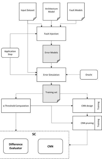
5 Smart Checker Design Methodology 51
5.1 Overview . . . 51
5.2 Training and Test Sets Generation . . . 53
5.2.1 Fault Injection . . . 54 5.2.2 Error Simulation . . . 55 5.3 α Threshold Computation . . . 57 5.4 CNN Architecture Design . . . 58 5.5 CNN Training . . . 59 5.6 CNN Pruning . . . 61 6 Case Studies 65 6.1 Case Study #1: Buildings Identification . . . 65
6.1.1 Structure . . . 65
6.1.2 Oracle . . . 67
6.2 Case Study #2: Land Segmentation . . . 67
6.2.1 Structure . . . 67 6.2.2 Oracle . . . 69 7 Experimental Evaluation 70 7.1 Introduction . . . 70 7.2 Baseline . . . 71 7.3 Experimental Setup . . . 71 7.4 Buildings Identification . . . 72 7.4.1 Fault Injection . . . 72 7.4.2 Error Simulation . . . 81 7.4.3 Difference Evaluator . . . 81
7.4.4 CNN Architecture Design and Training . . . 83
7.4.5 CNN Pruning . . . 87
7.4.6 Complete Hardened Application . . . 89
7.4.7 Design Effort . . . 91
7.5 Land Segmentation . . . 92
7.5.1 Fault Injection . . . 92
7.5.2 Error Simulation . . . 93
7.5.3 Difference Evaluator . . . 93
7.5.4 CNN Architecture Design and Training . . . 95
7.5.5 CNN Pruning . . . 99
7.5.6 Complete Hardened Application . . . 100
7.5.7 Design Effort . . . 101
8 Conclusions 104 8.1 Future Work . . . 106 8.1.1 Better handling the propagation of faults . . . 106 8.1.2 Employment of approximate replicas . . . 107
List of Tables
3.1 Generated Confusion Matrix . . . 41
7.1 Description of the Error Models . . . 74
7.2 Correlation of the Error Models to the Application steps -Buildings Identification Application . . . 75
7.3 Difference Evaluators Characteristics – Case Study #1 . . . . 81
7.4 Faulty Images Management for different α Values for the THR step . . . 82
7.5 Faulty Images Management for different α Values for the SHA step . . . 82
7.6 Faulty Images Management for different α Values for the AGGR step . . . 83
7.7 Faulty Images Management for different α Values for the R&C step . . . 83
7.8 Execution times of different SCs architectures – Case Study #1 . . . 85
7.9 Performance of different CNN architectures for the R&C step 85 7.10 Performance of different CNN architectures for the THR step 86 7.11 Performance of different CNN architectures for the SHA step 86 7.12 Performance of different CNN architectures for the AGGR step 87 7.13 Intermediate Comparative Analysis . . . 87
7.14 CNNs Execution Times – Case Study #1 . . . 88
7.15 Checkers’ Execution Times – Case Study #1 . . . 89
7.16 Performance of the SCs using the pruned CNNs . . . 89
7.17 Fault Management Scheme Performance – Case Study #1 . . 90
7.18 Design Methodology Phases times – Case Study #1 . . . 92
7.19 Faulty Images Management for different α Values for the Step 1 94 7.20 Faulty Images Management for different α Values for the Step 2 94 7.21 Faulty Images Management for different α Values for the Step 3 95 7.22 B block architecture for Step 1 – Case Study#2 . . . 96
7.24 B block architecture for Step 3 – Case Study#2 . . . 97 7.25 Execution times of different SCs architectures – Case Study
#2 . . . 97 7.26 Performance of different CNN architectures for Step 1 – Case
Study #2 . . . 97 7.27 Performance of different CNN architectures for Step 2 – Case
Study #2 . . . 98 7.28 Performance of different CNN architectures for Step 3 – Case
Study #2 . . . 98 7.29 Intermediate Comparative Analysis – Case Study#2 . . . 98 7.30 Performance of the SCs using the pruned CNNs – Case Study
#2 . . . 99 7.31 Checkers’ Execution Times – Case Study #2 . . . 100 7.32 CNNs Architecture Design and Execution Times – Case Study
#2 . . . 100 7.33 Fault Management Scheme Performance – Case Study #2 . . 100 7.34 Design Methodology Phases times – Case Study #2 . . . 101
List of Figures
2.1 Duplication with Comparison (DWC) scheme . . . 22
2.2 Triple Modular Redundancy (TMR) scheme . . . 23
2.3 General scheme of an image processing application . . . 24
2.4 An example of convolution . . . 24
2.5 Example of image processing application . . . 25
2.6 Examples of applied convolutional filters. . . 26
2.7 Example of Sequential CNN . . . 28
2.8 Example of Non-Sequential CNN . . . 30
3.1 Fault effects on processed images leading to usable (3.1(d)) or unusable (3.1(c)) images. . . 38
4.1 The hardening scheme . . . 44
4.2 The proposed Smart Checker module. . . 46
5.1 The SC design methodology. . . 52
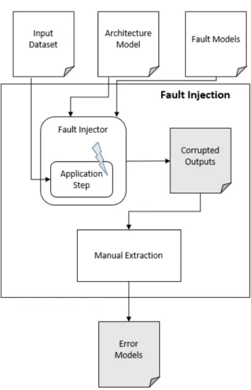
5.2 Scheme of the Fault Injection activity . . . 54
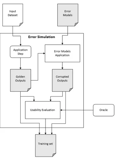
5.3 Scheme of the Error Simulation activity . . . 56
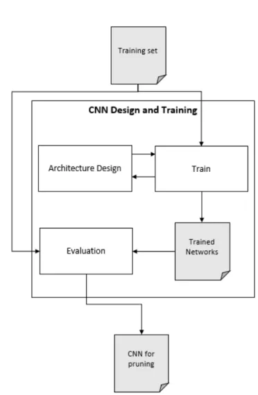
5.4 Scheme of the CNN Design and Training phase . . . 59
5.5 Algorithm for Automatic Pruning . . . 64
6.1 Examples of input and output images of the Case Study #1. 66 6.2 The structure of the Buildings Identification Application. . . 67
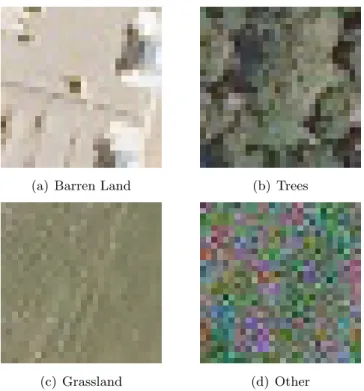
6.3 Examples of classes for Case Study #2. . . 68
7.1 Examples of LLFI outputs for the Sharpening (S) step. . . 76
7.2 Examples of LLFI outputs for the Sharpening (S) step (con-tinued). . . 77
7.3 Examples of LLFI outputs for the Sharpening (S) step (con-tinued). . . 78
7.4 Examples of LLFI outputs for the R&C step. . . 79
Abstract
Traditional fault detection/tolerance approaches introduce relevant costs to achieve unconditional correctness during data processing. For example, the classical Duplication with Comparison (DWC) approach achieves fault de-tection by duplicating the system and discarding data as soon as any error occurs, while the Triple Modular Redundancy (TMR) approach triplicates the system and achieves fault tolerance by means of a voting scheme. How-ever, many application environments are inherently tolerant to a certain degree of inexactness or inaccuracy. In this thesis, we focus on the practical scenario of image processing in space, a domain where faults are a threat, while such applications are very often not safety-/mission-critical and are inherently tolerant to a certain degree of errors. We first propose a shift from the concepts of corrupted/uncorrupted the concept of usability of the processed image to relax the traditional requirement of unconditional cor-rectness, and to limit the computational overheads related to reliability. We then introduce our new flexible and lightweight fault management scheme designed for application environments where inexactness is tolerated up to a given limit. The new scheme is based on the DWC approach but employs a flexible checker module that is able to deal with inexactness generated by faults and noise. A key novelty of our scheme is the utilization of Convolu-tional Neural Network (CNN)s to discriminate between usable and unusable images and reduce the costs associated with the detection and the manage-ment of faults. Experimanage-ments on two aerospace image processing case studies show overall time savings of 14.90% and 34.73% for the two applications, respectively, as compared with the baseline classical Duplication with Com-parison scheme. From the dependability point of view, the two hardened applications are able to correctly produce a usable output 99.7% and 98.4% of the times a fault occurs, which is well within acceptable margins in non safety-/mission-critical scenarios.
Sommario
I tradizionali approcci impiegati per il rilevamento e la tolleranza ai guasti in-troducono costi elevati per ottenere la correttezza assoluta durante l’elaborazione dei dati. Per esempio, il classico approccio Duplication with Comparison (DWC) permette di rilevare i guasti duplicando il sistema e scartando i dati non appena avviene un errore, mentre il Triple Modular Redundancy (TMR) prevede la triplicazione del sistema e permette di tollerare un guasto grazie ad uno schema di voto. Tuttavia, molte applicazioni hanno una intrinseca tolleranza ad un determinato grado di inesattezza. In questa tesi, ci concen-tiramo sullo scenario pratico dell’elaborazione di immagini nello spazio, un ambiente in cui i guasti sono un pericolo, mentre applicazioni di questo tipo non sono critiche per la sicurezza o per la missione e possono tollerare alcuni tipi di errori. Il primo passo `e proporre un cambiamento dai concetti di cor-rotto/non corrotto al concetto di usabilit`a dell’immagine in elaborazione per poter rilassare i tradizionali requisiti di assoluta correttezza e limitare i costi computazionali relativi all’affidabilit`a. Successivamente, proponiamo un in-novativo e flessibile schema di gestione dei guasti progettato per applicazioni in cui le inesattezze sono tollerate entro determinati limiti. Il nuovo schema si basa sull’approccio DWC ma utilizza un nuovo modulo controllore in grado di gestire le inesattezze generate dai guasti e dal rumore. Una importante novit`a del nostro schema `e l’utilizzo delle Reti Neurali Convoluzionali per discriminare tra immagini utilizzabili e inutilizzabili e ridurre i costi asso-ciati al rilevamento ed alla gestione dei guasti. Gli esperimenti condotti su due casi di studio evidenziano un risparmio di tempo ottenuto del 14.90% e 34.73% per le due applicazioni, rispettivamente, in comparazione con il clas-sico schema DWC. Dal punto di vista dell’affidabilit`a, le due applicazioni irrobustite con il nostro schema producono correttamente un output utiliz-zabile nel 99.7% e 98.4% delle volte in cui un avviene un guasto, risultando in margini accettabili per scenari non critici per la sicurezza o la missione.
Acknowledgements
This research has been possible thanks to all the people that collaborated with me throughout the year I spent working on it and thanks to those who always supported me during my academic career. Firstly, I want to thank Luca Maria Cassano, Antonio Rosario Miele, Cristiana Bolchini and Erdem Koyuncu because we were able to collaborate and work as a team to bring this work to life. I want to thank my parents, who always supported me during my entire academic career, both at Politecnico di Milano and UIC. Despite all the difficulties that arose during those years, they never stopped encouraging me and making efforts to allow me to have a good education. Without them, all this would not have been possible. I also want to thank my friends, my girlfriend and all the people that I met during my years as a student. With them I spent good and bad moments, traveled, studied and even worked and this contributed to make me become the person I am now. Last but not least, I want to thank all the Polimi-UIC students for being part of this amazing experience.
Chapter 1
Introduction
Digital systems are nowadays widely employed in a variety of different con-texts and scenarios. Depending on the application, digital systems can be more or less critical for the success of the mission they are involved in and for the safety of people and other systems connected to it. Safety-critical sys-tems are those syssys-tems for which a failure or a malfunctioning could threat the safety of people that are around it or working with it, cause the loss or severe damage to equipment or severely damage the environment. Life support medical equipment like Cardiopulmonary Bypasses and Mechani-cal Ventilation Systems are examples of safety-critiMechani-cal systems, because a malfunctioning could pose a severe threat to the life of patients. Mission-critical systems are those for which a correct functioning is vital for the success of the mission that the overall system has to carry out. Further-more, there are several classes of systems (e.g., automotive and aerospace) where safety-/mission-critical applications and non-critical applications co-exist. For example, in the aerospace domain, the navigation system of a satellite is a mission-critical application while payload processing applica-tions are not [11].
Failures and malfunctionings, especially in particularly harsh environ-ments, are often caused by faults. Some systems are often subject to physical stress or exposed to radiations and therefore some of their components have higher chances to break down or go through a temporary state change (e.g. memory data corruption, electronic glitches). In a system that is executing an application, a fault can make the application deviate from its nominal behavior and it often results in crashes, timeouts or incorrect outputs.
For mission-/safety-critical applications, it is therefore mandatory to provide the desired level of reliability in the computation. To this end,
hard-ware or softhard-ware implementations of fault management mechanisms like Du-plication with Comparison (DWC) and Triple Modular Redundancy (TMR) are adopted to achieve fault detection and fault tolerance, respectively [50]. When employing these approaches, the system is duplicated or triplicated, respectively, and the outputs of the copies of the system are compared to determine whether a fault occurred or not and, in the case of triplication, mask it with a voting scheme. In some scenarios, however, also non safety-/mission-critical applications may require (possibly as a soft requirement ) fault detection/tolerance capabilities, because even if errors in the output do not compromise the safety of system, a usable output may still be required for the correctness of eventual subsequent computations. For example, pay-load systems in the satellite scenario often consist of image processing ap-plications [23]. Such apap-plications collect pictures from a camera, apply a pipeline of manipulating filters and transmit the result to a base station on the Earth, which will in turn use the received data for its own purposes.
Certain Image processing applications may have an inherent degree of fault/noise tolerance, because:
• Sensor and camera data, especially in harsh environments, are often affected by noise and some applications are by design able to deal with it or
• Some end users do not need to receive a perfect output to be able to correctly use it (e.g. when the end user is a human, which is by nature not able to catch errors beyond a certain level of detail [35], or when the output is a probabilistic estimate and small errors are still considered tolerable) [3] or
• Some applications can work with inputs that are incomplete or inexact up to a certain degree.
When considering such applications, commonly adopted classical fault detection/tolerance methods (e.g., the DWC) may produce worst-case con-servative results since they discard the processed data as soon as a single pixel in the output of the duplicated system differs. When the processed data is discarded a re-execution of the filter, or the entire application, is triggered, causing a waste of time. Indeed, in certain cases, the fault that affects the pipeline processing may cause the output image to be only slightly altered. The slightly-altered image may still be usable by the end user/appli-cation for a correct execution of subsequent processes. In such a scenario, it would be possible to continue the processing and transmission of the result using the slightly-altered image without any re-computation, thus saving
time/power [5]. Conversely, if the affected output image is heavily altered such that it is not usable by the end user or downstream application, it is crucial to be able to detect the fault and re-execute the processing as soon as possible to limit time/power overheads. The classical DWC scheme only detects if a fault has occurred or not. In such a context, however, deciding whether to discard or not an image based on the occurrence of a fault is not enough. At the opposite, it would be beneficial to be able to decide as soon as possible if the overall image is still usable by the end user/appli-cation to decide whether to discard it or not. To this end, it is required to perform a more in-depth analysis of the faulty outputs and determine the impact that the fault will have on subsequent computations and on the downstream application before taking a decision.
1.1
Goal
The goal of this thesis is to propose a time-efficient flexible fault manage-ment scheme that extends the classical DWC approach by exploiting the classification capabilities of Convolutional Neural Networks (CNNs) to dis-criminate between usable and unusable intermediate and final outputs. Our fault management scheme is particularly suitable for application contexts that are inherently tolerant to a certain degree of inexactness. When a fault causes an error, the effects are evaluated and only if deemed necessary the ap-plication is re-executed to mitigate the effects of the fault. Our new method aims at limiting the reliability-related overheads by avoiding unnecessary re-executions, thus saving time and power. While the proposed scheme is general, the core component realizing the flexible error detection strategy needs to be designed, trained and optimized specifically for the application under consideration. To this end, a design methodology is also presented, supported by a semi-automatic framework supporting the designer in the implementation of the hardened image processing application.
1.2
Summary
The classical Two-Rail Checker (TRC) approach relies on executing the program twice and restarting the computation in case any difference in the two outputs is found. TRC usually meets reliability requirements but also causes a non-negligible loss of time that can be attributed to unnecessary re-executions of the program. The aim of this thesis is thus to design a time-efficient and flexible fault management scheme that can be applied at
fine-grain level on pipelines of filters to reduce the amount of time spent on their unnecessary re-executions.
A new flexible module, called Smart Checker (SC), is introduced in sub-stitution of the TRC and is meant to be tailored for the specific application step it is protecting. The SC module takes as input the two outputs of the replicas of the application step it is protecting and outputs a value that indicates if forwarding the data to the next steps will lead to a final usable output or not.
A SC design methodology is proposed. Given the application step we are trying to harden, the semi-automatic design methodology allows to construct a SC that is specifically tailored for the application step.
The scheme is then applied to two different applications, that serve as case studies. Both the applications are divided in steps, a SC is specifically designed for each application step and the performance of the system that uses the SCs are compared to the ones of the classical DWC approach.
The two metrics that lead the whole design process are the amount of accepted not usable images and the average execution time of the hardened pipeline. Being it the amount of times in which the hardened system gives a wrong output, the number of accepted not usable images represents the reliability flaw. During the design process we must try to keep them low while trying to minimize the execution time. Results show an overall time saving of about 14.90% and 34.73% for the two applications, respectively, incurring a reliability-related penalty (not usable images that have not been discarded) of about 0.3% and 1.6%.
The thesis is organized as follows:
• Chapter 2 sets the basis of the thesis. It introduces the notion of fault and describes the different types of faults, gives an overview of CNNs and discusses the related work by comparing it with the approach we propose;
• Chapter 3 provides a motivating example, discusses the assumptions behind the proposed hardening scheme and details the baseline against which we compare, together with the employed evaluation criteria; • Chapter 4 describes the proposed hardening scheme and introduces
the Smart Checker, along with a detailed description of its components and possible configurations;
• Chapter 5 introduces the Smart Checker design methodology that is used to tailor the Smart Checkers specifically for the application steps they protect;
• Chapter 6 describes the two case studies;
• Chapter 7 reports all the experiments we carried out to design and test the scheme and provides an analysis of the results;
• Chapter 8 describes possible future work and concludes the thesis.
1.3
Outcomes
The final outcome of this thesis is a complete and novel hardening scheme. A detailed definition of the newly introduced Smart Checker (SC) module is given, together with a description of all the possible configurations it can have. The hardening scheme comes with a semi-automatic framework and a complete design methodology that can be employed to the the SCs required to harden an application.
An more immature version of the scheme that is proposed in this thesis has been published at the Design, Automation and Testing conference in Europe, 2019 (DATE 2019) [5], while the final version is now undergoing major revision for a publication on IEEE: Transactions on Computers.
Chapter 2
Background
This chapter introduces the key concepts that represent the basis of the work presented in this thesis. First we introduce the notions of fault and error, in particular focusing on Single Event Upset (SEU) and Silent Data Corruption (SDC). Then, we describe the classical hardening techniques that are based on the introduction of redundancies in the system, the overall structure of an image processing application, generally organized in a pipeline of filters, and we present the key concepts regarding Convolutional Neural Network (CNN) design, training and pruning. We conclude by reviewing the related work.
2.1
SEUs and SDCs
The interest in faults in microprocessors arises from the fact that safety-critical systems are part of everyone’s daily life (e.g. automatic cars, emer-gency self-braking systems on cars, etc.). Among the causes of faults we find the fact that semiconductor technology has been geometrically scaled to sizes that are in the order of the nanometers and that the used power voltages become lower and lower. Also, some systems are often subject to physical stress or work in environments that are particularly prone to caus-ing a fault. Among such environments we can find for instance aerospace applications, in which radiations are a threat and can cause a state change in the microprocessor’s registers or in data stored in memory.
We can distinguish faults in three main classes [10]: • permanent faults, characterized by irreversible changes;
• intermittent faults, which are usually caused by hardware instability. In general, they do not affect the system permanently but usually
signal that a permanent fault is likely to happen;
• transient faults, which cause a malfunctioning in the system and have temporary effect.
On one hand, the semiconductor manufacturing technology has signif-icantly reduced the risk of occurrence of permanent faults. On the other hand, technology scaling makes electronic circuits become more susceptible to radiations, crosstalk or other noise sources, which usually cause glitches in the circuit (i.e. transient faults) [33].
Faults due to radiation effects, which are very common in aerospace applications [38], are usually referred to as Single Event Effects (SEEs). SEEs can be divided in soft errors, that have a transient effect in the system, and hard errors, that have a permanent effect. This thesis focuses on a subset of soft errors known as Single Event Upsets (SEUs). Electrically, the most important consequences of SEUs include temporary data loss in memories and flip-flops, transistor latchup, and corruption of logic waveforms. The errors associated with SEUs usually do not cause system destruction and they can be recovered by rewriting the data [37].
When considering a microprocessor-based system running an applica-tion, SEUs may cause one of the following effects:
• Program crashes. The fault can cause errors (e.g. modify the value of a variable) that make the program assume unexpected behaviors, which can result in a crash. Unexpected program crashes can effec-tively be detected and handled by the Operating System;
• Program timeouts. As in the previous case, one possible unexpected behavior is the timeout. Unexpected timeouts can be detected by means of watchdog systems. If a program does not reach its end within the maximum allotted time the watchdog assumes that it is stuck in an infinite loop and terminates it;
• Silent Data Corruption. SDCs occur when the data the program manipulates (i.e. data stored in memory or registers’ values) are cor-rupted without the program or the Operating System detecting and correcting it themselves. In this case, the program that is being ex-ecuted can still correctly reach its termination, but will eventually produce an incorrect output. If a single instance of the program is executed it is impossible to determine whether the produced output is correct or not. The effects of SDCs can be detected by using re-dundancy, that means executing the program more than once and
comparing the outputs. More details about possible approaches are given in Section 2.2.
This thesis focuses on SDCs, since they are the most critical effects representing an hazard for the correct system behavior, and has the purpose of proposing a novel scheme designed to be able to deal with faults of this type.
2.2
Hardening Schemes
Many approaches that can be applied when designing dependable systems make use of redundancy. The basic idea is to have multiple instances of the system or some of its components whose results are compared to determine whether a fault has occurred and has caused an error or not.
Duplication with Comparison [39] is a widely used technique that makes use of redundancy by instantiating two identical and independent replicas of the system that needs to be hardened. The output of the two replicas is compared and if a difference is found, an error signal is raised. The Duplication with Comparison (DWC) technique can be applied to a variety of different scenarios. Depending on the application, the replicated modules can be processors, I/O units, memories, softwares, etc.
A visual representation of the functioning of DWC is given in Figure 2.1. In the figure, the same input is fed to two replicas of the same system (e.g. a program), namely Replica 1 and Replica 2. The outputs of the replicas are then compared, if they are equal a ok signal is raised and the output is correct. If a ko signal is raised it means that the execution of at least one of the two replicas was affected by a fault. There is no way to tell which one of the two replicas was faulty, therefore there is no guarantee about the correctness of the output.
Another commonly employed approach is Triple Modular Redundancy
Figure 2.2: TMR scheme
(TMR) [39], which makes use of three copies of the same system to achieve fault masking. The outputs of the three copies is fed to a majority voting scheme capable at detecting and mitigating possible fault’s effects. More precisely, under the assumption of a single fault at a time, two possible situations may occur:
• The three outputs are equal. In this case no fault has occurred or • Two of the three outputs are equal and one is different from the other
two. In this case there was a fault which affected one of the three copies of the system. By giving as output the value of the two equal outputs, this is the case in which the TMR scheme effectively achieves fault masking.
Figure 2.2 gives a visual representation of the Triple Modular Redun-dancy (TMR) approach. The system is triplicated and the final output is decided through a voter.
Generally, such schemes are implemented by means of space redundan-cies; i.e., multiple independent processing units are instantiated in the ar-chitecture to execute the same application to subsequently compare the results. Nonetheless, there is an alternative implementation based on time redundancy, where a single processing unit is used to execute multiple times the same application in sequence. It is worth noting that the former scheme is more robust and works for both transient and permanent faults, while the latter works only with transient faults, under the assumption that after each run of the application, the processing unit is reset to a error-free status. In this work, since we consider SEUs, we will adopt the time redundancy ap-proach. Moreover, in such a scenario, DWC can be coupled with a selective re-execution, triggered only at the detection of a fault.
Figure 2.3: General scheme of an image processing application
Figure 2.4: An example of convolution
2.3
Image Processing Application
Image processing applications are softwares that are designed to perform a set of computations on one or more input images to produce a desired output (e.g. a classification or segmentation). Image processing has a wide range of possible application scenarios, ranging from aerospace applications, where a satellite may need to process pictures it took before transmitting them to a base station, to end-user applications, in which a camera may simply need apply a sequence of photographic filters on a picture.
It is a common approach to image processing to represent an application of this kind as a pipeline of steps, or filters, where each step takes as input the output of the previous step(s) and feeds the next step(s) with its output. An general example is shown in Figure 2.3, while 2.5 reports a practical example. This approach is particularly convenient in this scenario because it allows better scalability and helps categorizing the operations and features extracted by each application step.
Modern image processing applications often make use of convolutions. A convolution is a mathematical operation that is applied on the input with the use of a kernel (or filter). The kernel slides on the input and for each position the output value is computed as the dot product between the kernel and the corresponding values on the input. Such operations are used
Figure 2.5: Example of image processing application
to extract features from the input. Furthermore, convolutions that make use of specific kernels present the nice property of being invariant to rotations, shifts and other types of transformations that can be applied on the input. Figure 2.4 reports an example of convolution. In the figure, the matrix on the left is an example of input of a convolution, the matrix in the middle is the kernel and on the right we have the result of the convolution. The displayed kernel is an example of sharpening kernel. The highlighted cells show an example of how the kernel slides over the input to produce the result. The highlighted value in the result matrix is in fact the dot product between the highlighted part of the input and the kernel. Unless a specific padding strategy (e.g. 0-padding) is applied the output is generally going to be smaller than the input.
Figure 2.5 shows an example of image processing application. In the example, the input image first goes through a sharpening convolution and then an edge detection kernel is applied. The feature extracted, containing information about the edges, is fed to a 3D reconstruction procedure together with the original input image. Edge detection is another well-known and widely used operation which is useful in several contexts [51]. The figure also reports an example of edge detection kernel.
Figure 2.6 reports an example of input and output of two convolutional filters. Figure 2.6(b) is the output of an edge detection filter (reported in Figure 2.5) that had Figure 2.6(a) as input. Figure 2.6(d) is, instead, the output of the sharpening filter when applied on Figure 2.6(c).
2.4
Convolutional Neural Networks (CNNs)
In this section we introduce the general concept of Neural Network, define CNNs and describe their functioning. Furthermore, we will also talk about CNN architectures and training and pruning procedures.
(a) Input image (b) Edge Detection Output
(c) Input image (d) Sharpening Output
2.4.1 Overview on the Convolutional Neural Network (CNN) Neural Networks are parametric mathematical models that are widely used to learn complex functions from data. Their concept and functioning takes inspiration from the the biological model of a neuron. In general, a Neural Network can take multiple inputs and produce multiple outputs of arbi-trary shape, which makes them adaptable to a variety of different problems [19]. The inputs of a Neural Network go through multiple layers of neurons, where every neuron of each layer performs a specific - parametric - operation (depending on the type of layer) on the input values and then applies its activation function. Neurons belonging to the same layer generally apply the same activation function. Moreover, Neural Networks can be trained through Batch Training and can also perform Online Learning, which al-lows them to work in several different scenarios [17]. Convolutional Neural Networks are a type of Neural Networks that has proven to work particu-larly well on problems for which the input is a matrix in which values are correlated among each other (e.g. pixels of an image). CNNs are based on the concept of convolutions. The input of a CNN goes through a number of convolutions and is processed in order to produce the output [25].
There is a number of different layers that can be used in a CNN. Some common examples are:
• 2D Convolutional Layers (from now on abbreviated as Conv2D). Such layer performs multiple convolutions on the input and extracts a num-ber of features. The parameters to be learned in a Conv2D layer are the coefficients for the convolutions it performs, which determine which are the features extracted by the layer;
• Max Pooling (from now on abbreviated as MaxPool2D). Given a pool size, such layers calculate the maximum value among windows of values in the input and outputs a matrix constituted by the maximum values of all the windows. MaxPool2D layers help reducing the dimension of the state space and push the model towards better generalization thanks to the fact that they present invariant properties to certain spatial transformations, such as small shifts and noise. A Max Pooling layer has no parameters to learn;
• Add layers, that perform value-by-value addition of the two inputs, which must have the same size. Add layers are often used in ResNets [20]. An Add layer has no parameters to learn;
Figure 2.7: Example of Sequential CNN
the number of neurons and their activation function. In a Dense layer each neuron performs a linear combination of the values of its input and then applies its activation function. The parameters to learn in a Dense layer are the coefficients of the linear combination performed by each neuron.
Other examples of operations that can be done on one or more feature maps in CNNs are Concatenation (concatenates inputs on a given dimension), Subtraction (performs value-by-value subtraction), Multiplication (performs value-by-value multiplication) and Matrix Flattening (conversion of a matrix to a 1D array). In general, any type of operation is allowed if it proves to work well on the particular application scenario.
2.4.2 CNN Architecture
Defining the architecture of a CNN means defining all the structural param-eters that are independent from training, which include the number, type and ordering of the layers and the properties of each layer. Different types of layers are characterized by different properties that can be customized (e.g. kernel size, activation function and stride in a Conv2D layer or pooling size in a MaxPool2D layer).
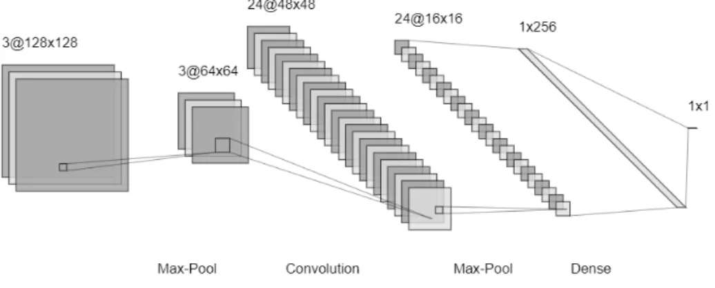
In Figure 2.7 we can see an example of sequential architecture of a CNN. A CNN is defined to be sequential if every layer has exactly one input and its output is fed to exactly one layer (except for the input, which is given, and the output, that is not fed to any other layer). In the example, the input has size [128, 128, 3] ([height, width, depth]). We can see that when processing the input, the height and width of the feature maps decrease while the depth (number of features extracted) increases. In the last layer
of the network, all the extracted low-level features are used to determine the output.
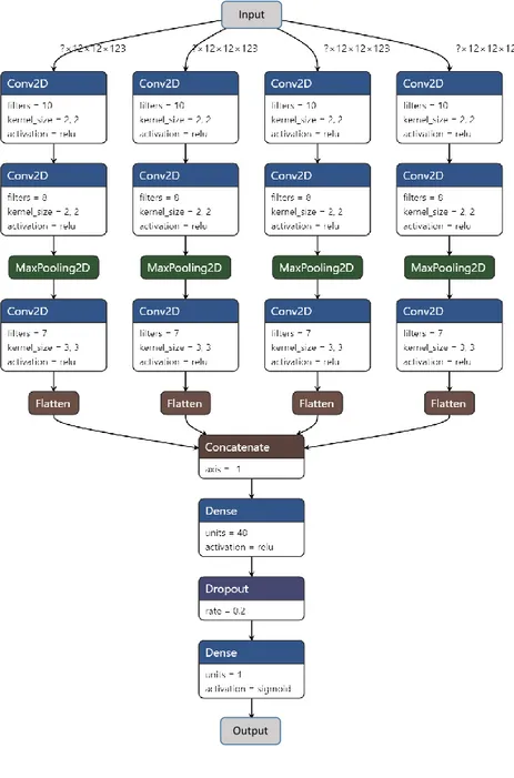
Figure 2.8 shows an example of non-sequential architecture of a CNN. A CNN architecture is defined to be non-sequential if there are layers that take multiple inputs or whose output is fed to multiple layers. In the example, the network takes as input a matrix of size [12, 12, 123] ([height, width, depth]). The input is processed independently by four identical branches, where each branch consists of two convolutional layers, followed by a max-pooling layer and another convolutional layer. The first two convolutional layers apply, respectively, 10 and 8 kernels of size [2, 2] ([height, width]) with Rectified Linear Unit (ReLU) as activation function, while the third convolutional layer applies 7 kernels of size [3, 3] with ReLU as activation function. The size of the pooling is [2, 2]. The output of each independent branch is flattened and concatenated to the others. The concatenated array goes through a fully connected (or Dense) layer and a last neuron with the Sigmoid activation function determines the final output. A Dropout layer is added to prevent overfitting during the training. It is worth noting that the Dropout layer remains inactive outside of the training process.
There is no rule to tell which is the exact architecture that works best on a certain problem. However, there is a set of empirical rules of thumb that one should keep in mind when defining an architecture:
• deep networks (more than 30/40 layers) can incur in some very well known problems, such as the vanishing gradient problem. Those prob-lems have already been widely addressed and so there are already sev-eral ways to solve or attenuate them [43]. One possible solution is to consider using ResNets [20] if the task requires a too complex or deep network;
• too fast dimensionality reduction generally leads to underfitting. Stack-ing too many consecutive or too close poolStack-ing layers or usStack-ing a poolStack-ing layer with a too large pooling size can cause the elimination of useful information too early, resulting in the fact that deeper convolutional layers can not exploit those information anymore. The definitions of too large or too close vary from task to task. On the other hand, reducing the size of features maps also reduces the time taken by the successive convolutional layers. Carefully chosen pooling sizes (and functions, such as Max or Average) may also help pushing the model towards better generalization.
Input
Output
2.4.3 CNN Training and Performance Evaluation
Training a Neural Network means finding the combination of parameters (e.g. the weights of the connections in fully-connected layers or values of the kernels in Conv2D layers) that minimizes a given loss function. The loss function is a function that indicates how well the model is tackling the prob-lem in exam and strictly depends on the probprob-lem itself [36]. The Gradient Descent [48] algorithm or one of its variants (e.g. Stochastic Gradient De-scent, Batch Gradient Descent ) [40] are used to minimize the loss function. When a new Neural Network is instantiated, all its parameters need to be initialized. A good initialization strategy allows the optimization process to be faster. Examples of initialization strategies are: i) zero initialization, in which all the weights are set to zero, ii) random initialization, in which the parameters are uniformly sorted and close to zero and iii) He-et-al ini-tialization, according to which the weights are randomly initialized keeping in mind the size of the previous layers [21]. While zero initialization has been proven not to work well, especially because of the mathematical na-ture of the Gradient Descent algorithm itself, the other two can represent good initialization strategies.
We define the train set as the set of data points that are used to train a Neural Network and the test set as the set of data points that are used to estimate the performance of the trained network. Samples in the test set must never be involved in training. Should this happen, the estimated performance would not be considered usable anymore.
Training a Neural Network is an iterative process. At every iteration, first the value of the loss function is evaluated on the train set and then the parameters of the model are updated by applying the update rule of the Gradient Descent algorithm or one of its variants. Training a Neural Network is therefore fundamental to allow the model’s parameters to change from their initial values to a combination of values that minimizes the chosen loss function. If the chosen loss function is suitable to the problem the Neural Network is supposed to exploit, minimizing it means learning the parameters that best represent the function we want to learn from data.
While training a Neural Network, particular attention should be paid to avoid overfitting on the train set. Overfitting means learning to make correct predictions on the training set without being able to perform as good on the test set or in the real world. There is a number of possible different causes for overfitting. Some examples are:
• training for longer than necessary a model that is more complex than the function we want to fit;
• the train set does not have enough samples or does not well represent the state space (e.g. the function is not well represented by the train set).
The application of Regularization Techniques helps avoiding overfitting. Some examples of such techniques are Early Stopping [7], Dropout [46] and Ridge Regularization [24].
2.4.4 CNN Pruning
Pruning a neural network means modifying it by removing connections, neurons or convolutions: this reduces the number of parameters and, as a consequence, memory occupation and execution time decrease. Expected improvements with respect to execution times, typically range from 3x to 11x [31].
In some contexts, reducing time and space overheads at the minimum is fundamental to achieve the desired performance. A blind approach would be trying to find the smallest Neural Network that is capable of tackling a certain task by training progressively smaller networks. Such approach is impractical due to the huge amount of architectural parameters and train-ing parameters that are involved. Pruntrain-ing techniques, instead, allow to progressively reduce the size of a network that has already proven to be able to tackle the task at hand, which helps saving a considerable amount of time. Pruning strategies directly aim at eliminating parts of the networks that are considered less important, making this process be faster than the blind approach approach. Therefore, the application of pruning techniques is necessary.
Pruning algorithms differ based on the criterion they use to identify the features to prune. Some examples are [31]:
• Average Percentage of Zeros (APoZ): The connections that are pruned in a certain layer are the ones that produce zeros more often than other connections, or more often than a certain percentage of times. This is applicable to all CNN layers that have ReLU as activation function (ReLU (x) = max(0, x)). The definition of the activation function implies that connections with a majority of negative weights and positive inputs or negative inputs and positive weights will tend to almost always provide a zero output as a result. A neuron that always gives the same result is most likely useless and can be pruned; • Sum of absolute weights (SoAW): When training a neural network, very few connections tend to have high-magnitude weights and many
connections tend to have very low-magnitude weights. The former are those that affect the final result the most, so it is possible to try pruning them without disrupting performance.
• Bruteforcing: Try removing every single connection, record the impact it has on the loss function and then effectively remove the connection that caused the smallest increase of the loss function. This approach is - theoretically speaking - the best one but it requires extremely high computational capabilities.
In all cases, after removing some connections, the network needs to be trained again to allow the remaining connections to adjust their weights and re-organize with respect to the loss of the removed parameters.
2.5
Related Work
The idea of adopting hardening schemes that relax some constraints has already been explored in various directions in the literature and at different levels of abstraction, from logic level to Register-Transfer Level.
Under the assumption of single fault, the use of TMR schemes with ma-jority voting guarantees the possibility of masking 100% of faults for a given circuit. However, a minimum area overhead of 200% is required because the system has to be triplicated. Various approximate/inexact TMR schemes have been proposed at the logic level [2, 42, 41, 16]. They mainly aim at reducing the area required by the hardened circuit by trading-off the pre-cision of the detection/mitigation scheme. For example, the classical TMR scheme is applied to a single-output combinatorial function, introducing two replicas that are smaller and eventually introduce errors. The subsequent majority voting scheme then masks such errors. The results proposed by [16] show that it is possible to achieve from 93.5% to 98.88% of fault masking with an area overhead that varies from 88% to 168%. The use of evolu-tionary approaches based on genetic algorithms has also been explored. [42] compares probabilistic approaches, that approximate a circuit basing on a probabilistic estimation of the error, against evolutionary approaches, which can provide completely different solutions that are hardly reachable using other methods. Experimental results demonstrate that the evolutionary ap-proach can produce slightly better solutions. The combination of the two approaches allows to explore the design space in depth. It is worth noting that evolutionary approaches have been applied to hardware optimization since when the research on such approaches has started. [29, 12] discuss
relevant applications in the field of electronic circuit design, diagnostics and testing.
A common point in the mentioned approaches is that they trade some precision to reduce the overheads introduced to satisfy the reliability-related constraints, which is similar to what we do in our approach. However, those approaches aim at reducing the area overhead of a TMR, while our main goal is to achieve fault tolerance while reducing the execution time of a system using DWC.
Different fault detection/management schemes have been considered in [9]. Starting from the DWC, [9] describes a low overhead, non-intrusive solution based on approximate circuits. The algorithm to synthesize approximate logic circuits is designed by the authors and provides flexible trade-offs be-tween area-power overheads and coverage. Two approximate voting schemes are presented in [8]. The first scheme is named inexact double modular re-dundancy (IDMR), is not based on triplication, thus saving overhead due to modular replication. This approach allows a threshold to determine the validity of the outputs. The second scheme combines IDMR with TMR. The validity of the three inputs is established and when only two of the three inputs satisfy the threshold condition. The two approaches and are in general devoted to reduce the size of the checker/voter circuits.
Common to these approaches is their focus on a limited number of bits or values that are manipulated, such that these proposal work at a low abstraction level, mainly tailoring the implemented function, therefore it is not possible to apply them to the application level, also considering the complete data rather than its elements. In fact, at application level the manipulated data can be constituted by millions of values (e.g. a RGB image with height 720 and width 1080 is defined by 2,332,800 values) that are possibly correlated among each other. Altough possible from a purely mathematical point of view, is it practically unfeasible to represent every output value as a function of so many input values to be able to apply the mentioned techniques.
Another set of approaches [45, 47], acting at Register-Transfer Level (RTL), is based on the reduction of the numeric precision in the DWC and TMR schemes. More precisely, the arithmetic units of the additional replicas and the checking/voting modules are designed to elaborate and check only the most significant bits of the values in the nominal circuit so that protection is provided only on a subset of the bits, those that are more relevant for the overall result of the computation. The technique, known as Reduced Precision Redundancy (RPR), is implemented with two identical copies of the reduced-precision version of the circuit we want to harden. RPR
is more difficult to implement that a classical TMR and requires to take some decisions at design-time, such as the number of bits of the approximation. RPR in some contexts has proven to achieve good performance with less than half of the cost of a TMR. The rationale is that the application context is inherently tolerant with respect to a certain degree of impreciseness in the results, due in reality to the presence of an error on the least significant bits. Our proposal stems from the same consideration, but the application scenario we take into account does not allow for these techniques to be applied, being all parts of the image relevant in the same way.
An enhanced version of the same strategy working at RTL consists in replacing the classical checker in fault detection schemes with a comparison of the numerical distance between the outputs of the nominal system and the introduced possibly-approximate replica with respect to a given thresh-old. This approach proved to be suitable for Floating Point Unit [14] and for Digital Signal Processing circuits used in signal processing contexts [22, 44]. To some extent, these RTL approaches introduce the idea of usability of the slightly corrupted results exploited in this proposal. Indeed, although the authors state that in general their solution is applicable to the image processing context, there is no straightforward extension from their scenario based on the single scalar data to the image one. In this thesis we also switch from the concepts of corrupted/uncorrupted to usable/unusable, fol-lowing the same idea according to which it is possible to accept a slightly corrupted output, and provide an hardening scheme that is suitable for im-age processing applications. It has also been observed in different contexts that designing a system to provide an acceptable/usable output rather than the best-possible/correct output can yield significant gains in terms of the system’s implementation costs and complexity [27, 28]. The solutions are however not applicable to our scenario due to the entirely different settings. The preliminary work at the basis of this proposal has been presented in [5], exploiting a smart fault management scheme and introducing the usability concept. Following the same rationale of the previously cited work, the outputs of an application are here considered as usable/unusable instead of correct/corrupted. The approach employs CNNs to have an advanced checker capable of analyzing the effect of the fault on the final result of an image processing application. However, the CNN is invoked every time there is a single different pixel between two replicas due to the occurrence of a fault, and the CNN is basic, therefore limiting the performance benefits. Furthermore, in [5] the same CNN architecture is used in all the cases. This new proposal enhances that idea and introduces a flexible, tailored and optimized checker, defines the methodology and the software framework
to harden the application, achieving improved results with respect to such previous work. In this thesis we also give more more precise insights about the design space and all the parameters that have to be explored.
In this chapter we introduced the concept of fault and described different effects that SEUs can have. We also detailed the generic structure of an image processing application and described some relevant concepts about CNN design, training and pruning. The notions introduced in this previous sections will be employed in the next chapters to present the hardening scheme and discuss the benefits and drawbacks of employing it.
Chapter 3
Goals and Requirements
In this chapter we will present a motivating example for our idea, describe the working scenario and discuss the criteria we adopt to evaluate the pro-posed hardening scheme together with the baseline against which we com-pare our results.
3.1
Motivating Example
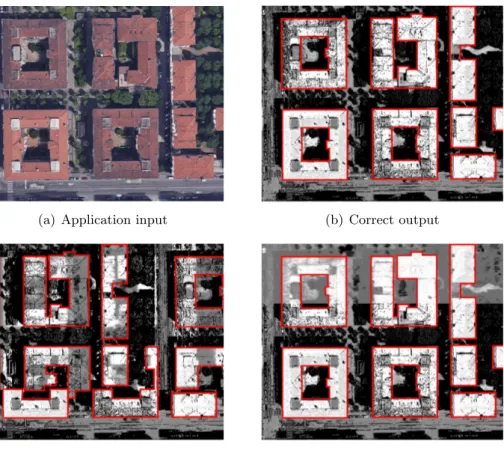
Let us consider the case of an image processing application consisting of several steps, running on a single-core microprocessor in an environment subject to radiation effects. Such radiations may produce Single Event Up-sets (SEUs) that affect the process(es) that manipulate the image, causing the overall application output to be corrupted. As an example, consider an application for identifying buildings in images taken from a satellite (Fig-ure 3.1(a)). This application produced heatmaps that highlight the presence of buildings, which are used by a downstream application that sets bounding boxes around buildings (Figure 3.1(b)). Should a fault occur during one of the steps of the processing and produce an observable error such that its intermediate result is corrupted, one of the two situations will hold on the final output image:
i) the impact of the fault is relevant, such as the one reported in Fig-ure 3.1(c), and the identified bounding boxes differ from the ones ex-tracted in a fault-free condition, shown in Figure 3.1(b). In this case, the error caused by the fault makes the heatmap unusable by the down-stream application. It is worth noting that the downdown-stream application is not going to be able to detect the problem, as it trusts that the data it is provided with are correct;
(a) Application input (b) Correct output
(c) Corrupted output: unusable (d) Corrupted output: usable
Figure 3.1: Fault effects on processed images leading to usable (3.1(d)) or unusable (3.1(c)) images.
ii) there is a visible effect of the fault, as shown in Figure 3.1(d), however the corrupted image is still usable leading to a final result (the bounding boxes) that is basically identical to the fault-free output or differs by an acceptable amount.
Our proposed approach discards a faulty image (intermediate data or final output) and performs re-computation only when the image is deemed unusable by the downstream application or end user. In general, every inter-mediate data produced by one of the application steps and the final output is classified into usable (U) or unusable (/U), and accordingly is discarded (D) or not (/D). The checkers of the intermediate outputs aim at predicting whether executing the rest of the pipeline and the downstream application will result in a usable output or not. The same reasoning applies to the checker that operates on the final output: it predicts if the downstream ap-plication is able to produce a correct result using the data. We thus move
from the correct/corrupted paradigm to the paradigm of usable/unusable, where inexactness is tolerated if it does not affect the usability of the final result. The definitions of usable and unusable is directly given by the end user or the downstream application.
While the difference between the correct and the corrupted is well-defined, the difference between the usable and the unusable is often context-related. As such, our proposed approach has a stochastic nature and may incur misclassifications where (i) a usable image is discarded (false positive), or (ii) an unusable image is accepted (false negative). Clearly, false posi-tives (D U) impact the effectiveness of the proposed approach, because re-computation is performed even when unnecessary. On the other hand, false negatives (/D /U) should be avoided because the flexibility of the methods reduce the reliability of the solution.
3.2
Working Scenario
In this thesis, we propose a software-based solution for achieving fault tol-erance in image processing applications executed on a general purpose em-bedded CPU, mitigating the effects of SEUs in the microprocessor memory elements or in the system memory. As a simplifying assumption, we be-gin by targeting applications that run in a single thread and single core fashion. More complex systems, including multi-cores, will be investigated in future extensions. In particular, the hardening scheme we propose only targets Silent Data Corruptions (SDC) under the single-fault assumption. Therefore, in the fault model we consider it can only happen that a Silent Data Corruption (SDC) causes one filter (or one checker) to output a wrong result.
Although the hardening scheme and can be applied to any application, in this thesis we mainly consider applications that can be divided in steps and therefore treated as a pipeline of subsequent filters, as this is a common approach in image processing applications.
The proposed scheme uses time redundancy to achieve fault tolerance, by exploiting and extending the Duplication with Comparison (DWC) scheme (shown in Figure 4.1) to detect the occurrence of a fault, and, when neces-sary, by performing a re-execution of the computation.
The solution we propose is general and can be applied to other hard-ware/software platforms, provided the fault/error relations are opportunely adapted, to enable the flexible identification of errors that can be tolerated. Future work will investigate this extension.
3.3
Baseline and Evaluation Criteria
We evaluate our scheme under various criteria. The proposed novel approach is an extension of the classical DWC technique, therefore we want it to maintain its flexibility and ability to adapt to different contexts and types of data that are manipulated. To this end, we adopt two case studies and we use one of them to fully develop the design methodology and the other one to test its generality and adaptability.
We evaluate the performance of the scheme in terms of:
• Time saving, measuring the reduction in the average execution time of the overall hardened system and
• Classification performances, measuring the number of samples that are correctly and incorrectly cassified.
Such performance indicators are calculated both at the end of the design process and during the design process itself, in order to make the best de-cisions on the components to use. More details are given in Chapter 5. As we aim at obtaining an improvement against the DWC technique, the latter represents our baseline.
The remainder of the chapter discusses more in details the baseline we chose and the evaluation criteria we adopt.
3.3.1 Baseline
As mentioned in the previous section, the baseline against which we compare our results is the classical DWC technique.
On one hand, DWC behaves perfectly in the case of fault-free execu-tion. In fact, a simple and not time-consuming check for equality in the two replicas is enough to determine that the execution was fault-free and avoid triggering an unnecessary re-execution. On the other hand, DWC is by nature a pessimistic approach: should a fault occur, a re-execution is triggered regardless of the intensity and position of the error.
The DWC approach does not resort on any intelligence and therefore it fails to adapt to the paradigm shift we propose, from the correct/corrupted paradigm to the usable/unusable paradigm. In fact, independently from the context and the considered types of errors, DWC is going to correctly classify all the correct outputs as usable but fails to distinguish whether a corrupted output is usable or unusable.
Such a conservative approach generates a number of useless re-executions and avoiding them would potentially improve the average recovery time of
Table 3.1: Generated Confusion Matrix
D /D
U %(D U) %(/D U)
/U %(D /U) %(/D /U)
the system. The approach we propose resorts on the computational capa-bilities of Convolutional Neural Networks (CNNs) and therefore are able to exploit a better classification. The use of DWC as baseline allows us to prove the benefits of our approach.
3.3.2 Evaluation Criteria
The two main evaluation criteria that lead the design process are two: 1. the classification performance, in terms of accuracy (number of correct
predictions with respect to the total number of samples evaluated) and, more precisely, by looking at the amount of errors of each type generated by every classifier (being it the Two-Rail Checker (TRC) or a CNN);
2. the execution time that the hardened system has when an error occurs, as we want it to be the lowest possible.
Every checker involved in the process exploits a binary classification problem. In fact, every checker outputs a discard (D) or not discard (/D) label for every input while the ground truth is instead expressed by means of the usability labels usable (U) and not usable (/U).
When an error occurs, comparing a prediction against the ground truth leads to four possible outcomes:
• Discarded Usable (D U) samples, where a usable image is erro-neously discarded. Even though this case does not impact the perfor-mance from the dependability point of view, it still causes a waste of time by requiring a useless re-execution;
• Discarded Not Usable (D /U) samples, where an unusable image is correctly discarded. In this case a re-execution is required and cannot be avoided;
• Not Discarded Not Usable (/D /U) samples, where an unusable image is mistakenly accepted. Even though a re-execution is required, the checker fails to detect it and therefore does not trigger it. This case represents the dependability flaw that we aim at minimizing; • Not Discarded Usable (/D U) samples, where a usable image is
correctly accepted. No re-execution is triggered in this case
The four outcomes are summarized in the Confusion Matrix, for which we provide an example in Table 3.1. Every Smart Checker (SC) that is involved in the design process is evaluated by means of a confusion matrix and the choices about the α thresholds and CNNs models to promote to the final steps are made basing on the amounts of /D /U errors.
It is worth noting that the classical DWC approach, by construction, cannot generate any /D /U and /D U. In fact, whenever an error occurs, it either correctly discards (D /U) or mistakenly discards (D U) the corrupted data.
Because the /D /U errors represent the reliability flaw of the scheme we aim at achieving the lowest possible execution time by minimizing the amount of such errors. Future work will investigate different trade-offs among the two quantities. The final average execution time of the sys-tem is calculated at the end of the design process by simulating the entire application with all its checkers.
In this chapter we first reported a practical example that serves as mo-tivation for this thesis and then we described the context in which the pro-posed scheme should be employed, together with the underlying assumptions it is built on. The chapter is concluded by detailing the evaluation crite-ria for an hardened application and the baseline scheme against which we compare.
Chapter 4
The Hardening Scheme
In this chapter we describe the hardening scheme and its functioning. The proposed scheme relies on the Duplication with Comparison (DWC) ap-proach and extends it. We introduce the Smart Checker (SC) module in substitution of the classical Two-Rail Checker (TRC) and describe in details its components and the possible ways which the module can be configured in.
4.1
Overview of the Hardening Scheme
The scheme we propose stems from the fact that in non safety-critical sce-narios the dependability-related constraints may be relaxed and not require absolute correctness of the output of a certain application. In such scenario, in fact, a corrupted application’s output may still be accepted if it is still usable by the end-user or downstream application. The usability of an im-age is directly defined by the end-user or downstream application. In fact, the downstream application may be intrinsically tolerant to noise or certain types of errors.
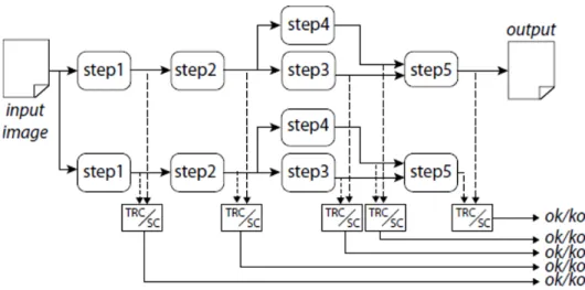
The scheme we propose relies on DWC strategy but substitutes the clas-sical TRC with the new SC module we introduce. Figure 4.1 shows the general idea of the scheme, reporting a duplicated pipeline where the out-puts of replicas of the same step are monitored by a TRC (as in the classical DWC approach) or by a SC module. Moreover, we couple the DWC with the re-execution technique in order to re-process a single step of the pipeline only when the SC detects a fault.
The classical TRC performs a bit-wise comparison, such that any single corrupted pixel leads the image to be re-processed. The re-processing is
Figure 4.1: The hardening scheme
performed independently of the impact of the corruption on the image, that is the number of corrupted pixels and effect on the usability of the produced output. The TRC module classifies all the corrupted images as unusable and therefore discards them. For this reason it tends to be too conservative when the dependability-related constraints are relaxed and some corrupted images are still considered usable.
At the opposite, the SC module we propose exploits the computational capabilities of Convolutional Neural Networks (CNNs) to perform a more advanced analysis of the step’s replicated outputs. Specifically, the CNNs predict if forwarding faulty intermediate data to the next application steps will still lead to a usable result or not. We employ the SC module because it has a higher classification capability than the TRC and therefore it adapts better to the task in which we want to correlate corrupted images to their usability.
Since we aim at reducing the recovery time, we adopt a fine-grain DWC strategy: the pipeline is divided in steps, replicated and the output of each application step is classified for a prompt (and possibly less expensive in terms of computational time) detection. An eventual re-execution only af-fects the interested parts of the application.
The proposed hardening scheme increases the complexity of the overall system but the main advantage it brings is the reduction of the execution time obtained by avoiding unnecessary re-executions of the application steps.
4.2
Granularity of the DWC
A fundamental point in this thesis is determined by the fact that we treat the applications as pipelines of smaller steps (filters). This is a common approach in image processing applications, as described in Section 2.3. The scheme is an extension of the classical DWC, therefore the application is duplicated.
From Figure 4.1 we note that it is possible to have application steps that take as input the same data (e.g. both steps 3 and 4 take as input the output of step 2) and also application steps that take multiple inputs (e.g. step 5 takes as input the outputs of steps 3 and 4).
There is no specific constraint to follow when dividing an application in steps. However, different divisions in steps may lead to different final perfor-mance. The application steps can perform different types of computation, have different execution times and manipulate data with different structures and sizes. Depending on the number and nature of the application steps an application is divided in, it is possible to work at different granularity lev-els. In particular, we work at coarse grain level when an application is not divided in steps or is divided in a very low number of steps compared to its total execution time and we work at fine grain level when an application is divided in a higher number of steps. Both the strategies present advantages and disadvantages:
• working at coarse grain level reduces the number of steps we have to harden, therefore reducing the number of SC modules we have to design or TRC modules we have to use. Since we have less SCs or TRCs, we introduce a smaller overhead in the system and the design time is reduced. On the other hand, if a step has long execution time, whenever we discard its output we have to re-execute the whole step because we do not know when the fault occurred during its first execution. This situation can result in the pipeline having a long recovery time when detecting and managing a fault. The worst case is represented by the scenario in which the pipeline is not divided in steps: should its output be discarded, the entire pipeline is re-executed twice;
• when working at fine grain level we divide the application in more steps, resulting in a higher number of SCs that have to be designed or more TRC modules that have to be introduced. In this case, the complexity overhead and the design time are larger than the case in which we have fewer steps. If there are more application steps with
input image
replica2
replica1
dif
ference
evaluator
CNN
pass/failresizing
exec if %diff <= α then return ok exec if pass then return ok return kook/ko
SC
resizing
%diff diffFigure 4.2: The proposed Smart Checker module.
shorter execution time, the recovery time when a fault is detected is going to be lower than in the coarse grain level case, provided that the execution time of the SCs is short enough.
The chosen granularity should, however, represent a trade-off between costs, in terms of design time and complexity, and benefits, in terms of performance and time savings.
For example, in Figure 4.1 if the output of step 4 is discarded we only have to re-execute this step and the related checker.
Another possibility could have been the one in which we divide the ap-plication in three steps (we could for instance consider steps 3, 4 and 5 as a unique step). In this case we would have two checkers less but if the output of this step is discarded we would have to re-execute it entirely and the recovery time would be the total execution time of steps 3, 4 and 5.
4.3
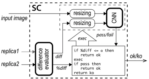
SC Architecture
Figure 4.2 shows the internal structure of the Smart Checker (SC) of each one of the DWC blocks depicted in Figure 4.1. The module receives the application input image and two replicas’ outputs and determines whether a re-computation is necessary (the output is a Boolean ok/ko signal). Given a set of inputs, the following situations may arise:
• the replicas’ outputs are identical (no error occurred),
• the two replicas’ outputs are slightly different (a fault corrupted one of them), or