Evaluation of new HTTP Adaptive Streaming algorithms: the clients’ and network’s perspectives

ALMA MATER STUDIORUM - UNIVERSITÀ DI BOLOGNA

Corso di Laurea Magistrale in Ingegneria Informatica

Dipartimento di Informatica – Scienza e Ingegneria

TESI DI LAUREA in

Reti di Calcolatori M

Evaluation of new HTTP Adaptive Streaming algorithms:

the clients’ and network’s perspectives

Candidato: Relatore:

Sergio Livi Chiar.mo Prof. Ing. Antonio Corradi Correlatori: Lucile Sassatelli, Maître de conférences Guillaume Urvoy-Keller, Professeur des universités Université Nice Sophia Antipolis

Abstract. Lo streaming è una tecnica per trasferire contenuti

multimediali sulla rete globale, utilizzato per esempio da servizi come YouTube e Netflix; dopo una breve attesa, durante la quale un buffer di sicurezza viene riempito, l'utente può usufruire del contenuto richiesto. Cisco e Sandvine, che con cadenza regolare pubblicano bollettini sullo stato di Internet, affermano che lo streaming video ha, e avrà sempre di più, un grande impatto sulla rete globale. Il buon design delle

applicazioni di streaming riveste quindi un ruolo importante, sia per la soddisfazione degli utenti che per la stabilità dell'infrastruttura.

HTTP Adaptive Streaming indica una famiglia di implementazioni volta a

offrire la migliore qualità video possibile (in termini di bit rate) in funzione della bontà della connessione Internet dell'utente finale: il riproduttore multimediale può cambiare in ogni momento il bit rate, scegliendolo in un insieme predefinito, adattandosi alle condizioni della rete. Per ricavare informazioni sullo stato della connettività, due famiglie di metodi sono possibili: misurare la velocità di scaricamento dei

precedenti trasferimenti (approccio rate-based), oppure, come recentemente proposto da Netflix, utilizzare l'occupazione del buffer come dato principale (buffer-based).

In questo lavoro analizziamo algoritmi di adattamento delle due famiglie, con l'obiettivo di confrontarli su metriche riguardanti la soddisfazione degli utenti, l'utilizzo della rete e la competizione su un collo di bottiglia. I risultati dei nostri test non definiscono un chiaro vincitore, riconoscendo comunque la bontà della nuova proposta, ma evidenziando al contrario che gli algoritmi buffer-based non sempre riescono ad allocare in modo imparziale le risorse di rete.

Contents

1 Introduction 7

2 The global network and its protocols 9

2.1 The Internet . . . 9

2.2 TCP . . . 12

2.2.1 Flow control . . . 14

2.2.2 Congestion control . . . 15

2.3 HTTP . . . 17

3 Streaming over the Internet 20 3.1 Video compression . . . 20

3.2 Video Streaming . . . 21

3.3 The principle of HAS . . . 24

3.4 Rate-based algorithms (RBAs) . . . 25

3.4.1 Interplay with TCP and client competitions of RBAs 27 3.4.2 Huang et al. algorithm . . . 30

3.4.3 Sabre . . . 30

3.4.4 Festive . . . 31

3.5.1 BBA-0 . . . 34

3.5.2 BBA-1: VBR encoding . . . 36

3.5.3 BBA-2: the start-up phase . . . 37

3.5.4 BBA-Others: instability and outage protection . . 38

4 Investigating BBAs performances: the empirical approach 39 4.1 Testbed . . . 39

4.2 Metrics . . . 41

4.2.1 QoE metrics . . . 41

4.2.2 Network metrics . . . 42

4.2.3 Competition metrics . . . 44

5 Assessment results of BBAs: the client and network perspectives 45 5.1 Quality of Experience metrics for a single client . . . 48

5.1.1 Constant bottleneck capacity . . . 48

5.1.2 Variable bottleneck capacity . . . 51

5.2 TCP metrics for a single client . . . 54

5.2.1 How CWND grows . . . 54

5.2.2 CWND idle reset . . . 55

5.3 Two competing clients . . . 58

5.3.1 Constant bottleneck capacity . . . 58

5.3.2 Variable bottleneck capacity . . . 61

5.4 Three competing clients . . . 62

5.5 Final remarks . . . 62

6 Conclusions 64

Chapter 1

Introduction

Like almost every piece of information, videos are seen as files in the digital world. In general we must download completely a remote file in order to open it. This is not true if we speak about video streaming: the playback starts potentially way before the end of the download; most people use it everyday, for example when using services like YouTube or Netflix.

Cisco [1] states that video streaming will be 79% of all consumer Inter-net traffic in 2018. Sandvine [2] declares that during peak hours in North America, Netflix and YouTube are together responsible for the 48.9% of the transfers towards the users. It is clear that video streaming is a topic with a rising impact on today’s Internet. Badly designed applications may pose problems not only to end users, but also to streaming providers and ISPs (Internet Service Providers).

Services have some indicators to measure user satisfaction; these indicators are gathered in the so-called Quality of Experience (QoE): a collection of metrics, usually not so easy to measure (mostly because of their subjective-ness), that evaluates the user satisfaction with the service. QoE for video streaming is believed to heavily depend on two factors: rebuffering events (when the video stops because of insufficient network throughput) and bit rate obtained (the more the bit rate is high, the more the images are clear, the more the user is satisfied).

Adap-tive Streaming (HAS) is widely used: it avoids rebuffering while at the same time getting a high bit rate. This is done by switching the bit rate on the fly while the playback is in progress, so as to absorb network fluctuations and obtain a high video quality.

Current HAS implementations measure the download throughput in order to chose the best bit rate sustainable, we’ll refer to this approach as rate-based; as highlighted by [3, 4, 5, 6] and many more, this method could suffer from some issues related to the interactions with the underlying layers.

Video streaming applications do not show immediately the data received to the user; instead, they keep a playout buffer of a variable length which absorbs the unreliability of the network, as there aren’t guarantees about the timing, even if the network is relatively stable (i.e. packets could arrive in bursts). An idea that comes from Netflix [7] suggests to choose the next bit rate using as input the utilization of this buffer, without trying to estimate the bandwidth at all, we’ll call this technique buffer-based. The authors demonstrated that with their strategy, the Quality of Experience increased, as the users obtained similar bit rates averages with less rebuffering events. The objective of this work is to dig on the two families of rate adaptation al-gorithms, and to compare some of the members of them, looking at metrics concerning QoE, network and competition between clients sharing a bot-tleneck; for the comparison we used VLC media player modified so to be capable of running different algorithms, on a testbed which permits network shaping, leveraging measurement tools to get the data from the clients, from the TCP stack and from the network equipment between the server and the clients.

In chapter 2 we provide an overview of the most important network tech-nologies; the context of this work is provided in chapter 3, detailing the prin-ciples of HAS and how the different algorithms cope with the problem. The methodology and the details of the implementation are presented in chapter 4; a discussion of the results obtained is given in chapter 5.

Chapter 2

The global network and its protocols

In this chapter we introduce the structure of the Internet and one of its most important protocols: TCP, we will then talk about HTTP, an application protocol built on top of TCP, that is responsible of the most part of the traffic on the Internet.

2.1

The Internet

Figure 2.1.1: ARPANET in 1969: the first four nodes of the future Internet

We can see the global network as an hetero-geneous set of randomly-interconnected ma-chines, where each of them can communicate with any other one, directly or by using one or more intermediate hops. An example, shown fig. 2.1.1, comes from the first stages of the Internet; we are in 1969, and this is the topol-ogy of ARPANET, the first computer network; each node in the picture is actually a couple of machines: the one represented by a circle is in charge of maintaining the links, while the other is the actual host to connect. This structure is

still used in the current implementation: the so-called routers are responsi-ble to manage the links and sort the traffic between end hosts.

ARPANET was at the beginning a military project, intended to keep under control the nuclear weapons in the USA territory even under a nuclear at-tack; under this conditions, it is easy to imagine how a part of the nodes could suddenly disappear. To raise the probability that every point remains accessible, it is necessary to add links in a web-like topology; having thus multiple possible paths between a given source and destination; for exam-ple in fig. 2.1.1, two of the three nodes on the left side could communicate between each other, even if the third one is down.

To exploit the multi-path topology, the information is split in packets, la-beled with source and destination, as Donald Watts Davies and Paul Baran suggested in the sixties [8]. The packets reach independently the destination without any kind of reservation of the path, and without any confirmation of the delivery; this is the most basic and lightweight communication mean on the computer networks; the implementation of this protocol on the In-ternet is called InIn-ternet Protocol (IP), with two versions that currently live together, as the transition is in progress: IPv4 and IPv6.

Data TCP data TCP header IP header Frame

header Framefooter Link

Internet Transport Application

IP data

Frame data

Figure 2.1.2: Encapsulation of data through the layers, as described in RFC1122[9]. Source: Wikipedia. An IP packet is made by an header

and a payload; the header contains source/destination pair, among other things, while the payload carries the ac-tual data to transfer. The machines are identified by their IP address, that is unique in the whole Internet.

IP is simple. This is one of its points of strength that permitted its diffusion: it is fairly easy to support it over any phys-ical mean of communication: copper, optical fiber, radio and so on. Fig. 2.1.2

shows the four layers of the Internet, as defined in RFC1122 [9]; IP sits in the middle of the “Internet hourglass”: many protocols carry IP packets as payload (Ethernet, Wi-Fi, UMTS...), and all standard protocols are built on top of IP.

On the transport layer, we find three different protocols that work over IP: • ICMP (Internet Control Message Protocol): useful for debugging

pur-poses, carries simple informations and error notifications.

• UDP (User Datagram Protocol): it adds the concept of port, giving thus the possibility to run simultaneously multiple network applica-tions on the same host, routing the data to the correct one. There is no guarantee concerning the correct delivery nor the order of the packets received.

• TCP (Transmission Control Protocol): in addition to ports, it adds some guarantees, such as delivery confirmation and packet order. It aims to establish a connection between the end hosts, exchanging IP packets both for control messages and user data.

Routing

The Internet is an heterogeneous set of different interconnected IP networks, where each independent network is connected to a number of other net-works; for each of them, the internal and external links are controlled by

routers, machines configured for this purpose (represented by a circle in

fig. 2.1.1). So the Internet could be seen as a graph, were the arcs are links and the nodes are routers. Our computers and servers are then connected to these routers, and all the data we exchange pass through the graph to reach the other peer. The links have in general different performances, due to physical reasons and depending on the quantity of data crossing them. Be-cause of these differences, a router could see bursts of traffic coming from a high speed link and going to a lower speed one; this is why, for each output port, the routers maintain a buffer so to have a queue of outgoing packets that empties at the link’s speed. When the amount of data flowing towards a link keeps having an unsustainable rate (higher than the capacity of the same link), this buffer could reach its limit; in this case, the router is forced to drop the subsequent packets; and the link is congested.

Without a specific mechanism to regulate traffic and avoid congestion, we could expect the most part of routers out-of-order and no communication possible across the Internet. For this reason, we need a mechanism to avoid congestion and ensure, as much as possible, a fair allocation of the available bandwidth; two approaches are possible: manage the traffic on the routers, or make the end hosts to send the data at a convenient rate. For practical reasons, the second approach was adopted at the first steps of the Internet and bundled inside TCP, under the name congestion control.

As the memory price decreases faster than how the link speed increase, the buffers tend to be oversized, especially on cheap, not-well-designed equip-ment; an excessive buffer size yields bufferbloat: the packets sits on the buffer, waiting to be routed for a time way longer than expected. This turns into an important issue in some fields, such as VoIP calls, on-line games or e-commerce web sites.

2.2

TCP

TCP was first defined in RFC793 [10], as “a connection-oriented,

end-to-end reliable protocol designed to fit into a layered hierarchy of protocols which support multi-network applications. The TCP provides for reliable inter-process communication between pairs of processes in host computers attached to distinct but interconnected computer communication networks”.

TCP by sending IP packets, establishes a connection between two end hosts and exchange data in a reliable way. The two involved peers have different roles, as the model is service-user: one acts as a server, exposing an open

port that accepts TCP connections, the other as a client, sending a special

packet to request the communication.

The connection is initiated by the client that sends a “synchronization packet”, SYN, as in fig. 2.2.1a; the server acknowledges the reception replying with a SYN+ACK packet; the client then ends the handshake sending a last ac-knowledgement, ACK. When the server receives this ACK, both sides con-sider the connection active, and identify it by the 4-tuple built with both

SYN

SYN+ACK

ACK

CLIENT SERVER

(a) three-way-handshake: the connection initialization DATA ACK PEER #1 PEER #2 R TT

(b) ACK mechanism: reliabil-ity and order

FIN ACK ACK PEER #1 PEER #2 FIN (c) four-way-handshake: the end of the connection

Figure 2.2.1: TCP phases

IP addresses and both TCP ports. From this moment on, there is no more difference between the server and client roles.

DATA DATA ACK PEER #1 PEER #2 R T O Figure 2.2.2: TCP, Re-transmission Time-Out A TCP connection, as seen from the upper layer, is

a streams of flowing data for each of the two op-posite directions. These two flows, to adhere to IP, must be split in packets, so to travel between end hosts over the network. Each data packet con-tains a sequence number that indicates its position on the stream, this ensures an ordered delivery to the upper layer even if the corresponding IP pack-ets arrived out of order. For each chunk of data sent, the receiver generate an acknowledge, that contains the next sequence number expected, confirming at the same time the reception of all the data; the time passed between the sent of the packet and the

recep-tion of the ACK is called Round Trip Time (RTT), as shown in fig. 2.2.1b. The reliability of TCP is obtained in a quite simple way: the memory area corresponding to a data packet is erased only when the matching ACK is received; if no ACK arrives, the sender will wait a Retransmission Time-Out (RTO), and eventually resend the packet (fig. 2.2.2).

FIN, that are confirmed by an ACK; the flag FIN announces to the peer

that no more data will be sent in its direction; the connection is actually closed when both sides closed their side (fig. 2.2.1c). TCP includes also a mechanism to abort a connection, by sending a reset request (RST).

2.2.1

Flow control

The data is split into packets in order to travel through the network, and every packet is acked, so to ensure reliability. Wait for the previous ACK before sending the next packet, anyway, is not so effective.

An example scenario: the two end hosts connected through a 10Mbit/s Eth-ernet link. For EthEth-ernet, the MTU (Maximum Transmission Unit, the max-imum payload size allowed) is 1500 bytes, the Ethernet header is composed by 14 additional bytes, total: 1514 bytes; IP and TCP headers are 20 bytes each; so the best-value TCP packet on Ethernet carries 1440 bytes of user data. The time to transfer this packet will be 1.2 milliseconds, and the ACK could be delivered 50 microseconds after (excluding the computation time at the destination); but we have to take into account also extra delays, for instance caused by the speed of light: if our link is 1500km of wire, we have to add 5 milliseconds; the total time passed between the send of the packet and the reception of the ACK is 11.2ms, with an average through-put of about 1Mbit/s: ten times less the actual bandwidth of the underlying medium. There is a number of other reasons that could cause delays, includ-ing: the other peer isn’t processing the packets because of high load, the data packets or the ACKs are stuck in queues on the intermediate routers. To obtain better performances, TCP sends more than one IP packet at a time, allowing a certain number of unacked packets. This receiver window (RWND) is moved forward as ACKs arrive, so to maintain the number of

in flight packets equal to its size.

As a first strategy, the window must be sized to not overflow the receiver’s buffer, as there is no point in sending data that the other peer can’t process; for this reason, the TCP header contains a field to specify the amount of

free space on the receiving buffer. The sender will limit the transmission to this amount of bytes, and update the window size to the advertised value on every received packet (ACKs included).

2.2.2

Congestion control

The mechanism presented above is useful to limit traffic end-to-end, not considering the status of all routers relaying the traffic; the main goal of congestion control is to avoid overloading the intermediate network equip-ment and links, while letting the machines dynamically get their own fair share of the available bandwidth. The sender keeps a congestion window (CWND), in addition to the receiver window of flow control; the effective number of allowed unacked packets will be the min(RW N D, CW N D). This CWND starts from a predefined size (initial window). The sender will fill this window sending as fast as possible, it will then stop waiting for ACKs. When an ACK arrives, the window size will be increased, and one or more new packets will be sent. Conversely, the window will be decreased when a loss is sensed (suspect congestion), i.e. when one packet remains unacked while its successors are, or when the ACK does not arrive after a certain timeout.

The exact behavior and the precise amounts for increases and decreases de-pends on the chosen algorithm (for instance, in Ubuntu 14.10, 13 differ-ent algorithms are available to be plugged into the kernel); although, some guidelines are given in RFC5681 [11].

Slow start and congestion avoidance

MSS (Maximum Segment Size) is the maximum allowed size for the TCP payload, it depends on many factors, and its rationale is to avoid fragmenta-tion at the lower layers; the transfer of a big file, for example, will be divided by MSS and produce a number of TCP packets.

DATA ACK PEER #1 PEER #2 DATA ACK DATA ACK R TT R TT R TT Figure 2.2.3: TCP slow start, how the CWND grows.

RFC5681 [11] recommends to set the initial win-dow to a low value (between 2×MSS and 4×MSS), and set a variable named ssthresh (slow start thresh-old) to an arbitrarily high value; when the current CWND value is less than the slow start threshold, the slow start algorithm is used, otherwise

conges-tion avoidance is selected.

When in slow start, for every ACK received, the CWND will be increased by a MSS, so the result-ing congestion window is doubled after an entire CWND sent and acked, or an RTT (see fig. 2.2.3); in this phase, the window grows exponentially to try to get to the maximum value quickly.

Congestion avoidance slows down the growth rate to linear: the increment for each ACK will be MSS×MSS/CWND, thus an MSS for each RTT;

this slow increase is meant to adapt to the channel bandwidth in a graceful way, avoiding high congestion.

What happens upon loss

The first and most naive congestion control algorithm is named Tahoe; it uses a timeout to determine the existence of a loss: if the ACK is not received before the expiration of the RTO, it will be considered a loss. The ssthresh will be set to half of the current congestion window, and the congestion window will be reduced to 1 MSS.

Stepping back to a very low CWND will suddenly drop the speed of the transfer, and moreover there are some more hints that could drive to good decisions without waiting for the RTO, in particular duplicate ACKs (DU-PACKs): if a packet is lost, for each subsequent packets delivered, the re-ceiver should produce a duplicate ACK of the last in-order packet received (that is equivalent to ask for the missing packet).

TCP Reno exploit this information to improve the recovery performances: at the third DUPACK, it will resend the requested packet (without waiting for the timeout), halve the CWND and set the slow start threshold to the same value, thus avoiding the slow start phase and reacting as soon as possible, before the RTO. If, anyway, the RTO arrives, the behavior of Reno is the same as for Tahoe.

As said, there is a number of other possible behaviors, currently deployed on the Internet, that optimize the edge cases, or use other TCP options, such as selective ACKs (SACKs), a mechanism that aims avoiding the resend on already-received, out-of-order packets.

Congestion window behavior

In order to exploit the available bandwidth of a defined path, or to fill the

pipe, we intuitively need a certain number of in-flight bytes; this number

could be calculated by multiplying the bandwidth times the round trip time; this is called bandwidth-delay product, or BDP, and we expect the conges-tion window to tend spontaneously to this value. Conversely, we can affirm that the current value of CWND, specifying the number of in-flight bytes, indicates directly the instantaneous throughput of the corresponding flow. Moreover, when in congestion avoidance, the CWND grows linearly and decreases exponentially; this approach is referred also as additive increase

multiplicative decrease or AIMD. This strategy is vital in TCP, in particular

when many active connections compete on the same bottleneck: it is demon-strated [12] that eventually each actor gets the fair share of the medium. It is important to note that this process takes time, depending on the charac-teristic of the links and on the congestion control algorithms in use.

2.3

HTTP

HTTP stands for Hypertext Transfer Protocol; it was used since 1990, and its first version is defined in RFC1945 [13]; created to transfer HTML

hy-pertext files, it is now used with almost every kind of data.

HTML, Hypertext Markup Language, is a file format that permits to link different related documents; it introduces also a way to identify and locate this related content: URLs (Uniform Resource Locator), pieces of informa-tions specifying the protocol that must be used and other protocol-specific data to obtain the document; HTML recommend but not enforce the use of HTTP. The applications that fetch and render HTML pages are called web

browsers.

An HTTP URL is in the formhttp://servername/path/to/file.html, where servername indicates the IP address or the hostname (mnemonic name, from which the clients will find the IP address) of the server, and path/to/file.html is the name of the document; to retrieve the docu-ment, the browser will open a TCP connection to the server at port 80, and send:

GET path/to/file.html [optional headers]

The server will then reply with some headers, specifying details about the file, such as the format, the modification date, etc., followed by the docu-ment requested. The connection is then closed.

HTTP is stateless, as the connection is established to download a single file, and no track is kept along the transfers; the cookie mechanism adds the concept of state in HTTP, by inserting a piece of information in the headers in both directions.

The currently most deployed version, HTTP/1.1 (defined in RFC2616 [14]), introduces a number of new functionalities. One of them, particularly useful for performance, is theconnection header: when set to keep-alive, the TCP connection is not closed right after the transfer, and could be used for the next request; reusing the connection has two great advantages:

• reduces the latency of the order of one RTT: a new TCP three-way-handshake is avoided,

• reuses the old congestion windows, already tailored for the path be-tween server and client.

Another functionality introduced in HTTP/1.1 is pipelining: the client could pack multiple requests without waiting the corresponding responses, which will be sent sequentially by the server in the same order; this approach speeds up the transfer of multiple resources hosted in the same machine. A new version of HTTP is defined in RFC7540 [15], dated 2015; HTTP/2 adds some interesting capabilities, helpful to gain some milliseconds in page load:

• header compression: depending on the transferred contents, the HTTP headers could have a non-negligible share of the whole download; • parallel transfers: concurrent HTTP requests and responses could be

run over the same connection;

• server push: a mechanism that allows the server to send unsolicited data, predicting a future request, for example if an HTML document includes some images (even though an image could be embedded di-rectly inside the HTML code, usually it is kept on the server as a sep-arate file, with its own URL), the server could assume that the client will need them soon, and push them right after the document.

HTTP/2 is widely supported by the major web browsers, but not yet exten-sively used on web sites, as it requires an update of both the infrastructure and web development community.

Chapter 3

Streaming over the Internet

The context of this work is characterized in this chapter: it starts presenting how videos are represented in digital form, continuing with video streaming and HTTP Adaptive Streaming, explaining then the basics of rate-based al-gorithms and their drawbacks, followed by a description of the buffer-based algorithms.

3.1

Video compression

A video file contains separately the audio and the images, because they are digitalized using different strategies.

The audio is converted by taking the value of amplitude of the signal at reg-ular intervals; this sampling has to be done in the order of thousands of times a second, so to respect the Nyquist-Shannon sampling theorem, that estab-lish the minimum frequency at which an analog signal must be sampled so to be reconstructed from its digital form without distortion; in particular, if the original signal is limited below a frequency fM, the sampling frequency

must be fs > 2fM. Human hearing works in the range 20 − 20.000Hz, so

to reproduce accurately a sound, fs must be greater than 40.000Hz.

The images are first split into a number of little squares, called pixels, in a grid with previously defined size, called resolution, for example 1280x720;

then, each of these pixels is saved extracting the value of three colors: red, green and blue; this procedure is repeated on a predefined frequency, called

frame rate, for example 50 times per second.

Sound and images are compressed individually, using codecs. A codec is a piece of software (or hardware, in some cases) responsible for compressing or decompressing the media stream; a common parameter that a compress-ing codec accepts is the bit rate, representcompress-ing the average number of bits that should be used to store a second of the content.

In a multiplexed video stream, the images would use much more space if compared to sounds; so from this moment on, for simplicity, we’ll hypoth-esize that videos don’t contain audio streams.

In particular, compression algorithms start from the assumption that a signif-icant part of frames is similar to their predecessors, dividing thus the frames (or parts of frames) in two main categories: key frames and delta frames. Key frames are stored independently, while delta frames contain only the differential part needed to transform the previous frame in the current one. As a consequence, the bit rate used depends on the motion of the video itself and changes along the content; codecs with this characteristic are called VBR (Variable Bit Rate).

3.2

Video Streaming

Video streaming is a technique to deliver video contents to the users through the network. When we say streaming we mean that the user starts enjoying the contents as soon as possible, before the transfer itself is completed. For example, watching a movie of 120 minutes on-line could mean downloading a 1.5GB file through a 10Mbit/s link, which means that the transfer will last about 20 minutes. But, given that the video data is spread sequentially on the file, there is no need to wait for the complete download before starting to display the movie to the user: the show could begin almost instantly.

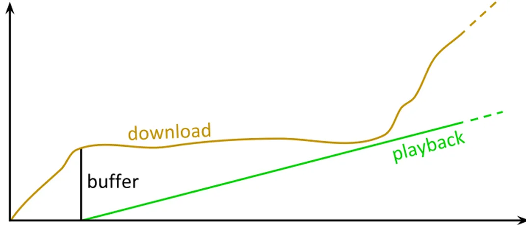
As the network (the underlying medium) does not provide guarantees about bandwidth nor delay, it is not a good idea to show immediately the contents to the user: if for some reason the data is delayed, the playback would freeze until the bytes arrive. It is then crucial to store temporarily the contents in a

buffer, so to absorb brief network fluctuations.

Figure 3.2.1: Video Streaming

This buffer will have a minimum and a maximum length. When its size is below the minimum, the player will wait for more data from the network (this is called prefetch phase); while when its size becomes more than the maximum, the player could ask the server to pause the transfer (in some implementations, this decision comes from the server), and resume it later, when the buffer depletes. This last behavior is called ON-OFF, and these bursty short transfers could break some assumptions in networking proto-cols, TCP in particular, and thus generate some problems to the underlying infrastructure.

Currently, the preferred protocol to transfer video files is HTTP, for conve-nience reasons: it is the standard for transferring web pages, so firewalls and network equipment are already well-shaped to work with it. In partic-ular, video providers should be able to rely on Content Delivery Networks (CDN): groups of servers put in geographically strategic locations, in order to be as near as possible to end users; the use of HTTP imposes little or no

changes to existing CDNs.

Quality of Experience

Given a service, the QoE is the quality level, as perceived by the human user. This is of course a subjective indicator, that can only be estimated. There is anyway a set of well defined objective metrics that are believed to have a direct impact on QoE.

Concerning video streaming, these are the main factors supposed to influ-ence QoE, ordered by importance:

• Rebuffering events: when the network throughput is not high enough, the buffer runs out, the playback stops, and the user must wait for the new data before the playback could resume. This downtime is con-sidered to be the most annoying issue in video streaming. Intuitively, these events happen when the throughput is lower than the bit rate, for a long period of time, depending on the buffer size and the ratio between throughput and bit rate.

• Video quality: as said, a video could be encoded at different bit rates (and with different codecs), the lower the bit rate, the lower the size of the resulting file, but also the lower the quality of the video; the lower the quality, the less the human eye will be able to see details on the im-ages. Of course, also the user’s device impact on this metric: smaller screen resolutions are not capable to display properly high video qual-ity, so it is possible to obtain similar perceived quality with lower bit rates.

• Startup delay: as said, the playback does not start before the prefetch

phase, while the user’s desire is to start the show immediately. It

should be noted that lowering artificially this delay (i.e. enforce a smaller buffer) could trigger rebuffering, especially if the bandwidth is not well higher than the bit rate.

3.3

The principle of HAS

The main goal of HTTP Adaptive Streaming is, clearly, maximize the Qual-ity of Experience. In particular, the target is to get a high video qualQual-ity, while avoid rebuffering events. This objective could be pursued by changing the bit rate of the video during the playback, on the fly, reacting to network fluctuations, adapting to the currently available bandwidth. It is worth to note that every change of the bit rate during the playback could disturb the user, thus impacting negatively on the QoE, especially if it is done often or if the bit rate jump is considerable (if the bit rates are relatively close the user could not even note the switch).

The main implementations currently used are:

• MPEG-DASH : is the international standard published by the MPEG working group in 2012, as ISO/IEC 23009-1 [16].

• Adobe HTTP Dynamic Streaming: the Adobe’s version, supported in Flash Player and Flash Media Server, from version 10.1.

• Apple HTTP Live Streaming: Apple’s implementation, part of Quick-Time and iOS, supported since iPhone 3.0.

• Microsoft Smooth Streaming: on the server side, it is an IIS (Inter-net Information Services, the HTTP server developed by Microsoft) Media Services extension; on the client side, various software devel-opment kits are available, compatible with Windows, Apple iOS, An-droid, and Linux.

These implementations differ for the codecs used and the specific file for-mats, but the general structure is shared: the video is split in segments (or chunks) with a fixed duration (in general between 2 and 10 seconds); these segments are then encoded at different (2-8) bit rates. A manifest file will hold all these complementary informations (bit rates, exact durations, URLs...). The client could decide to change the selected bit rate between the downloads.

Figure 3.3.1: HTTP Adaptive Streaming

It is worth to remember that the nominal encoding bit rate is not dutifully re-spected by the codec, when the compression is VBR: the instantaneous rate depends directly on the motion present on the video contents; this is clear in fig. 3.3.1, where the segments have all equal duration but the resulting file sizes differ.

3.4

Rate-based algorithms (RBAs)

The easiest and most intuitive way to adapt the bit rate to the network is to estimate the current bandwidth to base the choice. Proprietary adaptation algorithms are not identical between each other, but in general, the predic-tion is heavily based on the measured throughput during the previous down-loads. As an example, in [4, 5] we can find a simplified algorithm believed to mimic Microsoft Smooth Streaming client:

The player keeps two metrics related to the bandwidth: A, the throughput of the latest downloaded chunk, and ˆA, the running average of A. The value of ˆA, after the download of the segment i, is:

ˆ A(i) = ( δ ˆA(i − 1) + (1 − δ)A(i) i > 0 0 i = 0 with δ = 0.8.

We assign to each available bit rate an index, from the lowest to the highest. φcurdenotes the currently selected bit rate index. The player downloads the

first segment with φcur = 0, the lowest bit rate.

The next candidate profile φ is obtained by: φ = maxni : bi < c × ˆA

o

where c = 0.8 is used to absorb encoding and bandwidth fluctuations. φcur

is updated following this algorithm:

if φ > φcurthen

increase φcur by one

else if φ < φcurthen

decrease φcur by one

else

no action

Figure 3.4.1: HAS states Moreover, the player have two

dif-ferent states: buffering and steady

state. While in buffering phase, the

player continuously downloads seg-ments, until the buffer reaches a pre-defined size (30 seconds). It then stops downloading and switches to

steady state, in which the buffer size

is maintained almost constant: a new segment is downloaded after the com-plete playback of the current one. This generates the well-known ON-OFF

behavior: the player downloads a segment then it stops for some time, then

it downloads a new segment, then it stops, and so on. The duration of ON and OFF periods depends on the ratio between the selected bit rate and the throughput: the former indicates how fast the data is consumed, while the latter denotes the speed of new arrivals. For example, if the throughput is twice the bit rate, the two periods are likely to be equal (fig. 3.4.1);

con-versely if the throughput and the bit rate are similar, we don’t expect to see OFF periods.

The importance of ON-OFF behavior becomes clear if we think that: • It is not given that user’s device has enough memory to keep the entire

file. Think about an entire movie stored in RAM: this is not sustain-able, as is would consume for example, half of the available memory. • More importantly, network resources are expensive, so it is essential to avoid wastes as much as possible; the user could abandon the playback in any moment, so there is no point in downloading a big amount of data.

Real world clients would have more elaborate approaches. For example, it is reported that some of them integrate current buffer size in the behavior: they became more conservative when the buffer is low, and bet more when it is in a healthy state.

3.4.1

Interplay with TCP and client competitions of RBAs

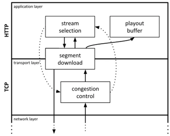
Figure 3.4.2: Rate based algorithms: interac-tion between control loops

The algorithm explained above does its best to estimate the available bandwidth, but maybe that is not the answer to the question which bit

rate should I chose? [3]. In

prac-tice, the stream selection we intro-duced is a control loop (fig. 3.4.2), which has as output the next bit rate, as input the measured throughput, and internally a mechanism that ig-nores completely what is happen-ing on the lower layers: in fact, by choosing the bit rate, it will

impact on the next measured throughput value, re-impacting then on the next decisions. The reason is the existence of another control loop, running on the transport layer: TCP congestion control.

Interactions between loops

Each time the player asks for a new segment using HTTP, a new transfer over TCP will be made from the server to the client; as said, the CWND di-rectly controls the throughput of TCP transfer, and the rate-based algorithms depend directly on the throughput, so the two control loops (stream selec-tion and congesselec-tion control) behave as a “nested double feedback loop” [4], something notably hard to predict.

The bit rate adaptation mechanism does not (and it is not supposed to) have access to the CWND value, also because they are located on the opposite sides of the communication: respectively the client and the server. So to measure the throughput, the client simply calculates the average throughput of the current segment, dividing the segment size by the time spent to down-load it. TCP, in the meantime, continuously changes the transmission rate trying to dynamically adapt to the fair share of the medium; a strategy that actually works well for long transfers, but does not guarantee optimal results for short transfers: upon a loss (or even without losses), the CWND could drop, and because of the length of the transfer, there wouldn’t be the time to grow back to a good value. This could unnecessarily force the stream selection to a lower profile. The impact of the losses on throughput is well explained in [6], where The the impact of a single loss on a segment transfer is analyzed, depending on the position of the lost packet relative to the begin and end of the download.

The lower the bit rate, the smaller are the sizes of the segments, the harder becomes make the CWND grow, as reported in [3] while studying the effect of a long flow competing with an HAS session. The authors detailed the bad cooperation between the side TCP flow and the HAS ON-OFF behavior, and tried to find some viable solutions.

Competition between RBAs clients

Table 3.1: Estimation inaccuracy for competing HAS players [5]

Moreover, it is worth to note that bandwidth estimation uti-lizes data taken only when a download is in progress. Ta-ble 3.1 [5] spots some peculiar cases of possible errors when two competing clients in steady

state share the same bottleneck

link with capacity C. When is

steady state, as said, the player

shows an ON-OFF behavior to keep the playout buffer as con-stant as possible. This could

generate strange scenarios in which the intermittent measurements yield in-sidious results.

• In the first example, player 1 downloads segments that are a little bit bigger than the ones downloaded by player 2. In this particular config-uration, player 2 will experience correctly half of the capacity of the link, while player 1, because of the fraction of time it was downloading alone, will measure more. This overestimation could drive player 1 to wrong bit rate decisions.

• The second case is an example where the players are downloading in a mutually exclusive fashion. In this case, they will both wrongly mea-sure the full link capacity, and so they are likely to be pushed towards a higher bit rate, in which the segments will be bigger; this is obviously unsustainable, and the players will eventually step back to a lower bit rate.

• The last example shows the best case: both players are getting half of the capacity, their estimation should be correct.

It is noteworthy that overestimation is not always an issue: if the error is neg-ligible compared to the distance between the available bit rates, no switch would be triggered; algorithms usually have a safety margin that prevents this, among other inconveniences.

3.4.2

Huang et al. algorithm

In [3], Huang et al. propose some modifications to a rate-based algorithm so to get better rates when a competing long flow shares the bottleneck link. The authors first reproduced a commercial HAS video player, then intro-duced these variations:

• Less conservative: increased the aggressiveness from the initial c = 0.6 value of their baseline algorithm to c = 0.9; TCP guarantees in any case that the client don’t get more than the fair share.

• Better filtering: instead of calculating the moving average, the authors used medians and quantiles; considering the 80thpercentile the vulner-ability to outliers is greatly reduced.

• Bigger segments: by requesting five segments at once, it’s possible to let TCP reach the optimum CWND size, improving the throughput and the decision taken by the algorithm.

3.4.3

Sabre

In [17], Mansy et al. analyze the bufferbloat effects caused by HAS, stating that it could easily add a delay of one second or more in residential con-nections. The proposition aims to minimize the impact on the buffers by limiting the amount of in-flight bytes; this could be done on the client side shaping the TCP receiver window, an effect that could be obtained by:

• HTTP pipelining: not waiting the end of the previous download before asking the next segment; if the receiver buffer is empty, the RWND

will be at its maximum, and the next transfer will start with a burst of packets, causing bufferbloat; keeping the HTTP pipeline non-empy make the RWND controllable.

• Reading the receiver buffer at a specified rate: in order to smooth the buffer fluctuations, the buffer must be emptied at a target_rate similar to the corresponding video bit rate; the throughput will follow, avoid-ing thus bursts of data.

As the throughput will be then measured by the client to choose the next bit rate, it is important to not limit it too much. Because of that, the algorithm works in two states, depending on the current buffer level:

• Refill:

if the buffer drops below refill_thresh,

target_rate = λ × Rh, with λ > 1, where Rh is the maximum bit rate;

• Backoff:

if the buffer exceeds backoff_thresh,

target_rate = δ × R, with 0 < δ < 1, where R is the current bit rate.

The player will start in refill mode, download smoothly but anyway having the possibility to get the Rh. When the buffer reaches an high occupancy

value, the algorithm won’t stop downloading, but it’ll limit the throughput slightly lower than the current bit rate; the buffer will then decrease, until the refill_thresh is met, and so on.

3.4.4

Festive

Jiang et al, in [18], focus on efficiency, fairness, and stability on competing players. The proposed approach has these properties:

• Randomized scheduling: in order to avoid synchronized downloads which bias the measurements, as table 3.1 second case, the requests are anticipated or delayed, by randomizing the maximum buffer capacity.

• Stateful bit rate selection: as in table 3.1 first case, players selecting high bit rates will tend to see higher throughputs; the proposition is to use the current bit rate as a status for the selection, making the selection more aggressive if the current value is low and more conservative if it is already high; this could be easily done by letting the rate switches being frequent for low bit rates and sporadic for high bit rates.

• Delayed bit rate update: the previous point introduces instability; in order to limit the impact, the result of the stateful selection is taken as an advice, and a concrete choice is taken after calculating and com-paring the costs in term of stability and efficiency for both proposed and current bit rates.

• Harmonic mean: the bandwidth is estimated by calculating the har-monic mean of the last 20 transfers’ throughput; this mean is more ro-bust to large outliers, if compared to the running average; this is partic-ularly important as the randomized scheduler increases the possibility of encountering throughput outliers: the number of competitors could vary greatly between segment downloads.

3.5

Buffer-based algorithms (BBAs)

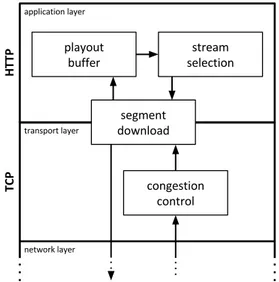
Figure 3.5.1: Buffer based algorithms: what we want to control is part of the loops

As [3] suggested, maybe it is not a good idea to try to measure the bandwidth when the first goal is to avoid the rebuffering events, while maximizing in the meanwhile the video quality delivered to the user. People from Netflix [7] agree: their data indicates that the throughput the single users get is far from be-ing constant, but conversely it is quickly variable, between 500kb/s and 17Mb/s, and so it is almost im-possible to try to predict what is go-ing to happen on the wire lookgo-ing directly at the past throughput. The idea proposed in [7] is: base the decision as much as possible on the playout buffer occupancy, as that is the main state variable we want to con-trol. This is not always possible, for example during the start up phase the buffer does not contain yet enough data to drive to a good decision, so at the beginning it is in some way necessary to measure the available bandwidth. There are four different flavors in this suggested buffer-based family:

• BBA-0: an initial version that draws the idea.

• BBA-1: variability of segment size is taken into account. The resulting choice is more tailored on the next segment to download.

• BBA-2: at the beginning of the playback, the buffer is empty, but this does not mean that the bandwidth is small. This version adds some simple throughput estimation to ramp up the buffer quickly in the start-up phase.

• BBA-Others: looking ahead to future segments, it tries to smooth the bit rate changes, believed to penalize the QoE.

3.5.1

BBA-0

Figure 3.5.2: BBA-0 rate map. Source: [7] The first algorithm of the family is

an initial version to draw and vali-date the idea. In fig. 3.5.2 is pre-sented the rate map, a function that ties the rate selection to the amount of data contained in the buffer; on the x-axis there is the playout buffer occupancy, measured as time, on the y-axis the video bit rates.

The buffer is split into three zones:

reservoir, cushion and upper reser-voir.

• The reservoir is meant to protect the buffer from draining; to under-stand its usefulness, it is important to add a couple of hypotheses: it is not possible to abort a download, and a different bit rate could be chosen as soon as the current transfer is completed. Thanks to the

reservoir, the player can safely finish downloading a big segment even

if the bandwidth drops (this is the meaning of safe area). When the buffer occupancy is between 0 and the reservoir size, the algorithm will recommend the lowest bit rate.

• The cushion is where the algorithm linearly choose a bit rate depending on the current buffer occupancy. There is not direct link between the decision and the experienced throughput.

• The upper reservoir allows the player to get the maximum bit rate; without it, the client would choose the highest rate only when the buffer is exactly full, while the whole area is actually safe enough.

In the paper’s implementation, segments are 4 seconds long, the buffer size is 240 seconds, the reservoir is set to 90 seconds, the upper reservoir to 24 seconds (10% of the total).

As said, when the buffer occupancy corresponds to the reservoirs, the player will get the respective bit rate. On the cushion, the algorithm first calculates the value of the f (B) function, which transforms the current number of sec-onds of video in the buffer in a continue value of bit rate (so normally, a bit rate that does not exist in the manifest file), then it follows these rules:

if Ratecur+1 exists and f (B) ≥ Ratecur+1then

increase cur by one

else ifRatecur−1exists and f (B) ≤ Ratecur−1then

decrease cur by one

else

no action

Where the bit rates available are ordered from the smallest to the greatest, cur denotes the index of the currently selected bit rate (zero-based), and

Rateindexindicates the specific bit rate value.

It is worth noting that in the BBA family, the ON-OFF behavior is mostly avoided: segments are downloaded continuously, and if the buffer keeps growing, the algorithm would barely select a higher bit rate. There is only one case in which the algorithms could stop downloading: if the buffer is full (but in this case the player is downloading segments from the highest bit rate).

3.5.2

BBA-1: VBR encoding

Figure 3.5.3: The size of 4-second chunks of a video encoded at an average rate of 3Mb/s. Note the average chunk size is 1.5MB (4s times 3Mb/s). Source: Te-Yuan Huang et al. [7]

As shown in fig. 3.5.3 the segment size is highly variable; as said be-fore, the VBR compression algo-rithms use an amount of bytes that depends on the motion of the spe-cific scene. A direct effect of this characteristic is that the download of two different segments (encoded at the same nominal rate) could take a hugely different amount of time, even if the network is relatively sta-ble.

The main implementations of HAS

do not carry the segment size in the manifest file; it is anyway not problem-atic to add these informations, this is way BBA-1 exploit these clues and use them instead of the average bit rates, as they are much more precise than the averages. Specifically, BBA-1 utilizes the segment size to build a dynamic

reservoir and to choose the next bit rate being aware of the real bit rate of

the corresponding segment.

In order to calculate reservoir size, we assume to have a client with an avail-able bandwidth equal to Rate0, and we expect this player to stream the

low-est quality without rebuffering events. This could be actually true if the instantaneous bit rate for all the segments is equal to the nominal average; as in that case the time to download any segment is equal to the segment duration; but the story changes if the segment has a higher or lower instan-taneous bit rate, and it is especially problematic if the segment size is above the average, as in this case the buffer will shrink. We need then to dimension the reservoir to absorb these bit rate variations.

The player defined above will have a playback free from rebuffering if its

play minus the amount of data that it will download, during the next X sec-onds. In the paper, X is set to the double of the buffer size: 480 secsec-onds. The reservoir is dynamically and continuously calculated, with extra safety bounds: between 8 and 140 seconds (respectively 2 segments and 35 seg-ments).

While the reservoir is now dynamic, the cushion doesn’t change its size; on the other hand, the rate map is substituted with a chunk map: with respect to the buffer occupancy, while in the cushion, the algorithm will choose a segment size, and not a rate; in this way the selection is more tailored to the specific instantaneous bit rate.

The upper reservoir follows the variations of the reservoir to keep intact the total maximum size of the buffer.

3.5.3

BBA-2: the start-up phase

At the beginning of the streaming session (or after a seek on the video), the buffer is empty; BBA-0 and BBA-1 fail interpreting this phenomenon as low-capacity network, and applying a conservative behavior; this is not always a good choice, as with some probability the network could safely give more. In these conditions, where the buffer does not hold informations, it is necessary to estimate the available throughput; doing so, it is possible to make the buffer grow faster in an initial phase.

In practice to ramp up in bit rates, the ratio between download time and playback time for the last downloaded segment should be bigger than a cer-tain factor. At the beginning, this factor is equal to eight, decreasing then linearly as the buffer grows up through the cushion. BBA-2 keeps staying in this start-up phase until the chunk map (BBA-1) gives a higher bit rate or the buffer starts decreasing.

3.5.4

BBA-Others: instability and outage protection

Figure 3.5.4: Chunk map increases

instabil-ity. Even if the buffer level and the mapping

function remains constant, the variability of segment sizes can make BBA-1 often switch between rates. The lines in the figure rep-resent the chunk size over time from three video rates, R1, R2, and R3. The crosses

rep-resent the points where the mapping function suggests a rate change. Source: [7]

There is still some issues running on that could cause problems to end users: Temporary network outages can show up for example on resi-dential ADSLs or because of Wi-Fi interferences, and the instability is introduced by the choice to rely on segment size in BBA-1. In this con-text, instability indicates how often bit rate is changed, and it is a direct effect of the variable segment size, as reported in figure 3.5.4.

Insta-bility has a bad impact on QoE, as

frequent bit rate switches could dis-please the user.

BBA-Others aims to both reduce

in-stability and protect from network outages, with two strategies:

• The reservoir is bound only to grow, but not to shrink; this helps keep-ing an extra amount of reservoir, useful in case of network issues, and stabilizes the bit rate selection, as the chunk map will move less fre-quently.

• Before choosing to a higher bit rate, the algorithm will look ahead to next segments, avoiding the switch if with the current conditions it would take the opposite choice soon. We could expect that the bigger the amount of look ahead, the more it will smooth the rate; in [7], the authors propose to look ahead to the same number of segments currently held in the buffer. Note that the rate change is not avoided if the chunk map suggested to decrease the bit rate, so to maintain a good resiliency to rebuffering events.

Chapter 4

Investigating BBAs performances:

the empirical approach

This chapter proposes a methodology to compare the families of algorithms: the testbed and the metrics.

Buffer based algorithms have been tested directly in the wild, through the Netflix service, for single client metrics, in [7], and it is demonstrated that they succeeded to decrease the impact of rebuffering events while obtain-ing almost the same bit rates in average as the rate based algorithm used at Netflix at the time. This work aims to compare the algorithms in a con-trolled environment, focusing on other metrics, representing the impact on the network and the competition between the clients.

4.1

Testbed

The testbed run entirely on top of VirtualBox, a hypervisor, orchestrated with Vagrant. The configuration files hold all the informations concerning the virtual machines (VM), in this way the set of VMs could be regenerated and automatically configured with a single command.

Each box in fig. 4.1.1 represents a virtual machine in the VirtualBox envi-ronment. There are different (virtual) networks between the VMs, so that the

Figure 4.1.1: The testbed

packets are forced to flow through the bottleneck emulation (bandwidth+de-lay).

HTTP Server

HAS protocols do not require particular server configurations for the Video On Demand part (this is not true for Live video streaming, that anyway is not our case), so the HTTP server implementation is a simple node.js instance that serves static files.

Bandwidth and delay

These two machines are meant to simulate the bottleneck. They both use

tc-netem Linux tool, from the traffic control suite to shape the traffic so to

emulate a link with given bandwidth and delay, respectively.

Clients

For simplicity, we preferred the Apple HTTP Live Streaming (HLS) proto-col. The clients run a modified version of VLC player1, so to behave like the simplified player in [4, 5]; the libcurl library was linked to allow the

reuse of the TCP connection between the downloads, and all the BBA fam-ily presented in [7] was implemented. The resulting application is capable to run different configurations by passing specific parameters as environment variables.

4.2

Metrics

The tests run on the testbed are classified by looking at specific metrics, concerning the Quality of Experience, the network utilization and the com-petition between the clients.

4.2.1

QoE metrics

As cited before, the important metrics regarding Quality of Experience, are:

rebuffering events, bit rate and instability.

Rebuffering events

This is the most important metric impacting QoE. A rebuffering event hap-pens when the player suddenly stops the playback, because the buffer got empty. Note that if a segment is not completely downloaded, it is not avail-able to the player.

To characterize the impact of rebuffering, we could:

• Count the number of rebuffering events in a session. This could be a good idea, but it is implicitly tied to other variables: video duration and segment duration. The first is pretty clear: the shortest the video, the less data to download, the less opportunities to have problems. For the second, if the playback continuously stops after each segment waiting for the next one to be downloaded, it is clear the the longer the segments are, the less the rebuffering events will be. It should be noted, also, that the cardinality of rebuffering events could be artifi-cially lowered, forcing longer waiting times.

• Calculate the rebuffering ratio: the idea here is to measure the fraction of time spent waiting for new data, dividing the sum of the duration of all the rebuffering events by the total duration of the session. In other words, it is the fraction of time while the player was in rebuffering state.

Bit rate

To evaluate the bit rate obtained by the clients, three metrics could be inter-esting:

• average bit rate: simply obtained by summing the nominal bit rate for each segment downloaded and dividing by the number of segments. • average relative bit rate: the average bit rate divided by the

bottle-neck capacity, so that measures coming from different tests (i.e. with different bottleneck capacities) could be compared.

• average quality level: the bit rates are not spread uniformly, but the higher the bit rate, the bigger is the distance with its neighbors. This metric takes the average of the indexes of the bit rates of the down-loaded segment and scales it as a percentage.

Instability

The metric for instability, as in [5], is obtained by dividing the number of bit rate switches by the total number of segments.

4.2.2

Network metrics

Congestion window

The congestion window (CWND) is the parameter that auto-adapt the TCP flows to the current network conditions. It is an important metric to

under-stand how the data is exchanged on the network. To capture the value, we used the kernel module tcp_probe.

Router buffer

The simulated bottleneck is preceded by a buffer, that is emptied at the rate imposed; this buffer has a maximum length and it grows and decreases as time passes, depending on the network activity; it is possible to poll traffic

control to get its current status.

As the maximum buffer capacity is not constant between the tests, we chose to take also the average value relative to the maximum.

Round Trip Time

We impose a static delay to the packets, but they could experience an ad-ditional delay, caused by the combination of the said router buffer and the bottleneck capacity. We recorded the average RTT perceived, relative to the base we enforced.

Link utilization

It is interesting to see how much of the bottleneck capacity is actually ex-ploited by the HAS flows. For this purpose we took a copy of the headers for each packet arrived and departed from the bandwidth VM, using tcpdump; sampling the time in hundredths of second, we then counted the number of packets, and bytes. We used these samples to obtain the network rate entering and leaving the bottleneck link.

4.2.3

Competition metrics

The metrics about competition denote various aspects that arise when the bottleneck is shared between HAS clients.

• bit rate unfairness: the absolute value of the difference between the two average bit rates.

• average bit rate unfairness: the difference between the bit rates di-vided by the bottleneck capacity.

• quality level unfairness: the absolute value of the difference between the two average quality levels.

Chapter 5

Assessment results of BBAs: the

client and network perspectives

This chapter presents a description of both the algorithms and the videos in-volved in the tests; a part of the results obtained follows, concerning single-client, two-clients and three-clients sessions, under different points of view: QoE, network and competition metrics.

Videos

Tests were conducted over two videos with peculiar characteristics: the first presents a constant segment size and four bit rates, the second is a real movie with high variability and eight quality levels.

Apple’s BipBop

For testing purposes, and to get the first results, it is useful to have a video without segment size variability (i.e. Constant Bit Rate, CBR). Some initial tests were run against a video with this characteristic, before switching to a real movie.

This video is the basic example for the HLS protocol, as provided by Apple1; it contains constant motion, so as a result, there is almost no variability in

segment size: even if the codec used is VBR. The entire run time is 30 minutes, with 181 ten-seconds segments (the last is 4 seconds long).

Available bit rates are:

• 232 kbit/s at 400×300 pixels, • 650 kbit/s at 640×480 pixels, • 1 Mbit/s at 640×480 pixels, • 2 Mbit/s at 960×720 pixels.

Big Buck Bunny

It is an open source movie, freely downloadable from the project web site2, re-encoded using ffmpeg3 to prepare HLS segments and manifest files. The video duration is about 10 minutes, 299 two-seconds segments. For the lowest bit rate, the biggest segment is 2.2 times the nominal average. Available bit rates are:

• 350 kbit/s at 320×176 pixels, • 470 kbit/s at 368×208 pixels, • 630 kbit/s at 448×256 pixels, • 845 kbit/s at 576×320 pixels, • 1130 kbit/s at 704×400 pixels, • 1520 kbit/s at 848×480 pixels, • 2040 kbit/s at 1056×592 pixels, • 2750 kbit/s at 1280×720 pixels. 2_{https://peach.blender.org/} 3_{http://ffmpeg.org}

Algorithms

Figure 5.0.1: Time-line of data ex-changed between the peers

These are the bit rate decision algorithms tested:

classic: inspired from the simplified player

in [4, 5]. The available bit rates are compared with the running average of the obtained throughput, multiplied to 0.8 as safety margin. This throughput is obtained by dividing the segment size by the time span between the start of the HTTP request and the end of the response.

classic_est: mostly as classic, but

measur-ing the throughput as the segment size divided by the time span between the first and the last received bytes. The difference between the two is shown in fig. 5.0.1: classic starts measuring the time at the beginning of HTTP GET, while classic_est at the beginning of the data stream.

Both classic and classic_est were tested with two different playout buffer sizes: 30 seconds, as in [4, 5], and 240 seconds, as for the BBA family.

BBA-0, BBA-1, BBA-2, BBA-Others: as defined in [7]. BBA-Others was

further modified halving the look-ahead window, to frame the impact of this mechanism on the metrics.

Tests performed

Various tests were run against both of the videos cited above, with different network configuration and different number of clients, on all the algorithms presented. We ran experiments with both constant and variable bottleneck capacity, with different router buffer limits and dropping policies, and with different delay values. Each experiment ran twice if one client was involved, four times otherwise, to ensure a good confidence interval on the results.

5.1

Quality of Experience metrics for a single client

5.1.1

Constant bottleneck capacity

BipBop

A batch of 20 different experiments, with fixed delay (200ms) and fixed bottleneck capacity (ranging from 300kbit/s to 2.2Mbit/s), was run twice. Concerning the rebuffering ratio, there is not a particular difference between the algorithms, but we clearly noted a divergence on the bit rate obtained: the average bit rate weighted on the link capacity got by BBAs is around 90%, while for RBAs it is less than 55%; two factors could explain this gap: • The highest bit rate is wrongly reported as 2Mbit/s in the manifest file (taken directly from Apple), while instead it is 1.5Mbit/s; this infor-mation, in buffer based family, is utilized only by BBA0 to build the rate map, but it does not have the same impact on the choice as for the RBAs.

• The rate-based algorithms stick to the highest bit rate below the sup-posed link capacity, while the buffer-based oscillate to between two bit rates as the current buffer occupancy suggests, taking sometimes an unsustainable bit rate and stepping back when needed, without impact on rebuffering. This second point drives the analysis to the instability: RBAs are around 1%, BBAs get obviously an higher value, 4%; this is not problematic, as 4% means 8 rate switches, in this 30-minutes video.