RESEARCH ARTICLE
10.1002/2014WR016237
On the control of riverbed incision induced by run-of-river
power plant
Simone Bizzi1, Quang Dinh2, Dario Bernardi3, Simona Denaro2, Leonardo Schippa3,
and Rodolfo Soncini-Sessa2
1European Commission, Joint Research Centre (JRC), Institute for Environment and Sustainability (IES), Water Resources
Unit, Ispra (VA), Italy,2Department of Electronics, Information, and Bioengineering, Politecnico di Milano, Milano, Italy, 3Engineering Department, University of Ferrara, Ferrara, Italy
Abstract
Water resource management (WRM) through dams or reservoirs is worldwide necessary to sup-port key human-related activities, ranging from hydropower production to water allocation and flood risk mitigation. Designing of reservoir operations aims primarily to fulfill the main purpose (or purposes) for which the structure has been built. However, it is well known that reservoirs strongly influence river geo-morphic processes, causing sediment deficits downstream, altering water, and sediment fluxes, leading to riverbed incision and causing infrastructure instability and ecological degradation. We propose a framework that, by combining physically based modeling, surrogate modeling techniques, and multiobjective (MO) optimization, allows to include fluvial geomorphology into MO optimization whose main objectives are the maximization of hydropower revenue and the minimization of riverbed degradation. The case study is a run-of-the-river power plant on the River Po (Italy). A 1-D mobile-bed hydro-morphological model simulated the riverbed evolution over a 10 year horizon for alternatives operation rules of the power plant. The knowl-edge provided by such a physically based model is integrated into a MO optimization routine via surrogate modeling using the response surface methodology. Hence, this framework overcomes the high computa-tional costs that so far hindered the integration of river geomorphology into WRM. We provided numerical proof that river morphologic processes and hydropower production are indeed in conflict but that the con-flict may be mitigated with appropriate control strategies.1. Introduction
Dams and reservoirs are essential for many human-related activities involving water management. Their purposes range from water allocation for irrigation, industrial and domestic supply to hydropower produc-tion, flood risk mitigaproduc-tion, land reclamaproduc-tion, and recreation. Regardless of their purpose, reservoirs affect the longitudinal continuity of fluvial water and sediment flow and alter the flood peaks and seasonal distribu-tion of discharges causing substantial geomorphological adjustment downstream [Kondolf, 1997].
A vast amount of literature has studied the effects of dams on river systems in terms of both geomorpho-logical and ecogeomorpho-logical responses [Poff and Hart, 2002; Gupta et al., 2012; Petts and Gurnell, 2005]. Dams affect the hydrological regime downstream primarily through changes in timing, magnitude, and frequency of high and low flows [Magilligan and Nislow, 2005]. Peak discharge downstream is generally significantly reduced. Sediment connectivity is altered by dams which trap a large amount of sediment load delivered from upstream. In response to the altered water and sediment fluxes, channel aims to establish a new equi-librium by a complex range of geomorphological adjustments which can include several steps and may take decades before reaching a more stable condition [Petts and Gurnell, 2005]. Channel changes can include alterations of the cross section, bed material (e.g., coarsening), slope, pattern, and bed forms. By trapping sediment upstream, reservoirs can often cause the river transport capacity to exceed the available sediment supply, creating a sediment deficit downstream [Grant et al., 2003], which in turn triggers river erosion both on the riverbed and the banks. This process can extend over hundreds of kilometers and last for decades.
Some frameworks have been developed to assess the effects of sediment trapping of dams on river channel processes [Grant et al., 2003; Burke et al., 2009]. Nevertheless, when planning dam operation rules only the
Key Points:
!Riverbed degradation included in MO
optimization of reservoir operation
!Surrogate modeling of a
hydro-morphological model by response surface
!Pareto-optimal solutions derived for
hydropower revenue and riverbed incision
Correspondence to:
S. Bizzi,
Citation:
Bizzi, S., Q. Dinh, D. Bernardi, S. Denaro, L. Schippa, and R. Soncini-Sessa (2015), On the control of riverbed incision induced by run-of-river power plant, Water Resour. Res., 51, doi:10.1002/ 2014WR016237.
Received 2 AUG 2014 Accepted 29 MAY 2015
Accepted article online 1 JUN 2015
VC2015. American Geophysical Union.
All Rights Reserved.
fulfillment of the main purpose (or purposes) for which the structure has been built is considered, often hydropower production or water supply. Few studies included the influences of dam operations on river processes [Wild and Loucks, 2014; Yin et al., 2014].
Multiobjective (MO) approaches can take into account a variety of societal needs affected by the dam man-agement from flood mitigation to water supply or environmental quality. MO methods have been adopted to provide decision makers and stakeholders with valuable tools to evaluate the consequences of alterna-tive operating rules from a variety of perspecalterna-tives [Castelletti et al., 2007; Yin et al., 2009]. These experiences have marked a significant progress in our ability to plan sustainable management of water resources and provided more comprehensive insights into how dams affect the fluvial system and the related ecosystem services. However, integration of fluvial geomorphological process into the planning of optimal operating rules remains very rare. Some authors implicitly addressed the issue by managing flashing floods to restore basic environmental functions [Dittmann et al., 2009; Wu and Chou, 2004; G!omez et al., 2013; Yin et al., 2014]. More recently, Wild and Loucks [2014] addressed similar issues at catchment scale, assessing the cas-cade effects of multiple dams in the Mekong basin on sediment connectivity. With the exception of a single example [Nicklow and Mays, 2000; Nicklow and Ozkurt, 2003], studies that have optimized dam regulations in order to minimize their impact on channel morphological adjustments downstream are absent. Never-theless, the operational value of this previous approach was limited. The model relied on a single-objective framework, i.e., considered the effect of operating rules on downstream riverbed incision, but neglected other objectives such as hydropower revenue or water supply as commonly addressed in a MO approach. Additionally, the framework did not provide daily operation rules, but focused on flood conditions, only. The lack of consideration of river geomorphology in MO water management in the scientific community is surprising, considering the recent interest for multiple, negative effects of dams on channel morphodynam-ics. One reason is in the currently limited capability for predicting fluvial geomorphological response on the relevant time scales [Brasington and Richards, 2007]. On the other hand, channel morphological alterations develop over time scales from decades to centuries, and many of these alterations were not foreseeable during the second half of the last century, when most of the dams have been built worldwide. Finally, it is unclear to what extent optimal operating rules accounting for fluvial geomorphology can reduce negative morphological effects.
Nowadays, running physically based (PB) models that simulate both hydrodynamics and riverbed evolution over extended spatiotemporal scales are feasible due to increased computer power [Langendoen et al., 2009]. These models could be suitable to derive detailed estimates of river morphological response to dam construction and regulation. Unfortunately, the computational costs of such a procedure are still too high to allow for integration into MO optimization routines. MO optimization routines need to evaluate an ele-vated number of different alternatives in order to identify the Pareto-optimal decisions [Castelletti et al., 2007]. The high number of required model evaluations makes the integration of PB river evolution models into MO optimization practically infeasible. Nevertheless, the computational burden associated to PB mod-els ranging from water quality to water distribution issues [see Razavi et al., 2012, and reference therein] is a common problem in MO water management. To overcome this limitation, PB models can be replaced by surrogate models that maintain key characteristics of the original model, but require only a fraction of com-putational effort. A range of surrogate models has been developed over the past decades, and are now widely applied [Razavi et al., 2012; Castelletti et al., 2012].
The aim of this contribution is to propose a modeling methodology of general validity for including riv-erbed degradation when designing optimal operating rules of reservoirs. Specific goals of this research are (i) testing the suitability of surrogate modeling, such as global Response Surface Methodology (RSM), to integrate a 1-D PB hydro-morphological model into a MO design problem to identify Pareto-optimal operat-ing rules of a HP plant; (ii) assessoperat-ing the feasibility and utility to account for the river geomorphic changes when planning optimal operating rules.
This paper analyzes the effect of alternative operating rules for Isola Serafini—a run-of-river HP plant on the River Po, Italy—where the downstream river reach is affected by a severe incision rate since 1960s. We implemented a one-dimensional PB hydro-morphological model to simulate the riverbed evolution over a time horizon of 10 years along a 112 km long river stretch. We then built a MO framework to assess the effects of alternative operating rules on hydropower revenue and riverbed incision, and finally provide
Pareto-optimal decision rules. We adopted the global RSM [Castelletti et al., 2010a] as surrogate modeling technique to embed the PB hydro-morphological model into the MO optimization framework.
We start from the case study description, and the introduction to the hydro-morphological model to facili-tate the following description of the control problem. The MO control problem is formulated and the main aspects of the (global) RSM are briefly recalled. Two alternative control schemes are proposed: a pure feed-forward control scheme (Scheme A) and a mixed feedfeed-forward-feedback control scheme (Scheme B). They are implemented for the case study and their performance is analyzed. We conclude with a discussion of potentials and limits of the proposed framework for future applications.
2. The Case Study: The River Po and the Isola Serafini HP Plant
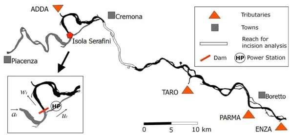
The case study of Isola Serafini (IS) run-of-river hydro-power-plant (HPP) in the Po valley (Italy) is presented in Figure 1. The Po is the longest river in Italy and runs for 652 km across the northern regions from the Alps to the Adriatic Sea, with a catchment area of approximately 70,000 km2. The River Po is widely
exploited, most of all as a source for irrigation in the fertile valley, but also as an important waterway. The present study focuses on a 112 km reach (see Figure 1) from Piacenza to Boretto, which includes the IS HPP. The power plant (Figure 1) is located 30 km downstream of Piacenza and has been operating since 1962. It consists of a barrage which diverts part of the incoming flow to four vertical Kaplan turbines (total installed power capacity 80 MW). The diversion channel was originally the result of a meander cutoff during the large 1951 flood and joins the main channel 12 km downstream of the diversion (Figure 1). The barrage has 11 sluice gates of equal width. Two gates feature a lowered bottom for sediment-scouring purposes. Six gates can be overtopped functioning as sharp-crested weirs. There is no room for water storage behind the bar-rage, except for short transitories during maneuvers, pondage is not a management option.
During the twentieth century, the middle-lower course of River Po has experienced a significant degrada-tion of the bed, a process that accelerated after the construcdegrada-tion of IS HPP, which altered the flow regime and created a sediment transport disconnection. There are also other human pressures affecting both sedi-ment supply and sedisedi-ment transport capacity. Among these, instream sand mining seems to be very rele-vant. Sand mining was very intense from 1950 until 1980. After that, stricter regulations have first reduced and then stopped the activity. Surian and Rinaldi [2003] state that instream mining increased from about 3 to 12 million m3/yr in the period 1960–1980, and then decreased to about 4 million m3/yr. The peak volume
(12 million m3/yr) is estimated to be not far from the assessed average annual sediment yield of the basin.
As consequence of riverbed lowering, several navigation and irrigation structures became unusable during low flow periods, e.g., harbor locks in Cremona, where minimum water levels decreased by more than 4 m from 1950 to 2000 requiring expensive interventions to rebuild locks or restore their functionality. The esti-mated costs of the new locks alone exceed e 40 millions [Bonomo and Luisa, 2011]. Other impacts include instability of, e.g., flood protections and infrastructures, and freshwater ecological alterations, for which eco-nomical appraisals are missing.
For all these reasons, IS HPP is a challenging case study to assess optimal operating rules that maximize hydropower revenue and minimize riverbed incision downstream of the plant. In particular, we analyze the effects of alternative operating rules over a time horizon of 10 years in terms of riverbed incision nearby Cremona. This reach has been significantly affected by riverbed degradation in the past and has a strategic role for navigation and flood defense. Our choice is also supported by the findings of Bernardi et al. [2013], which have shown that this reach is the most sensitive to IS operation. Toward this aim, we refer to a com-plete historical time series of water inflows from 1964 to 1973 recorded at Piacenza, and at the relevant trib-utaries. For this period, data are readily available and are suitable for this illustrative case study.
3. Modeling the System
3.1. Isola Serafini Operating Rules
The only objective of the IS HPP is electricity generation: its present operating rule aims at maximizing hydropower production. The water level upstream the dam is constantly kept at 41.00 m a.s.l. with a
maximum tolerance of 0.50 m. The production is stopped during floods for safety reasons. As previously recalled, no water pondage is allowed so continuity at the bifurcation is satisfied at any time.
The IS operating rule-curve is shown in Figure 2. A Minimum Environmental Flow (MEF) of 100 m3/s is
imposed, and the minimum design flow of the turbines is 200 m3/s. Hence, if the incoming flow a is lower
than 300 m3/s the turbined flow u is null, whereas when a is greater than 300 m3/s, all inflow exceeding the
MEF is diverted to the turbines until the plant capacity (1000 m3/s) is reached. For larger values of the inflow
a, the power station keeps working at its maximum capacity and all the additional discharge passes throughout the gates and flows into the meander. When the incoming flow a exceeds 4000 m3/s the
tur-bines stop working (u is set to zero) for safety reason, and to avoid upstream flooding, all the gates are fully opened to allow flood pass-through.
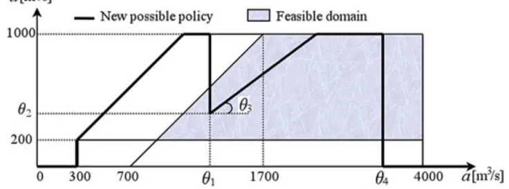
For designing the new operating rules, we consider the following class of piecewise linear operating rules such as the one defined by the bold black line in Figure 3:
u50 if 0 " a " 2001MEF u5minða2MEF; 1000Þ if 2001MEF < a " h1 u5minðh21h3% ða-h1Þ; 1000Þ if h1 < a " h4 u50 if a > h4 : 8 > > > > > < > > > > > : (1)
A specific rule within this class is defined by instantiating a four-dimensional design parameter vector h, the four elements of which are denoted as h1, h2, h3, and h4. The parameter h4is the discharge threshold
at which all the gates of the barrage are completely open. It primarily affects sediment supply to the downstream reach through the gates, while the other three parameters affect the transport capacity in the meander by reducing the discharge u through the turbines.
The present operating rule (in the fol-lowing named Business As Usual-BAU-rule) is a particular rule of this class and can be obtained by alternative instan-tiations of the parameters, for instance, h1& 300; h251000; h350; h454000:
(2) The vector h should be chosen within a feasible domain which can be extracted from the current operating
Figure 1. Scheme of the Isola Serafini and the stretch of the River Po analyzed.
rule, since it accounts for the physical constraints: the MEF, the minimum and maximum flow through the tur-bines, and the safety limit against flood risk. Moreover, previous studies on the Po River have shown that the sediment transport in the meander is triggered only when the discharge is larger than 700 m3/s [Rosatti et al.,
2008]. Taking care of all these condi-tions, the feasible set H (see also equation (13d)) is specified by 2000 < h4" 4000 900 < h1" h4 200 < h2" minðh12700; 1000Þ 0 < h3" 1 ; 8 > > > > > < > > > > > : (3)
and the corresponding operating rules lies within the gray area in Figure 3.
3.2. The Hydro-Morphological Model
To represent the riverbed evolution processes correctly at the reach scale over a 10 year horizon, and to avoid excessive computational times the choice fell on a one-dimensional mobile bed hydro-morphological model. The model was first introduced in a previous work by Schippa et al. [2006]. We adopted the version of the model presented in Schippa and Pavan [2009], and adapted it to the specific requirements of the case study.
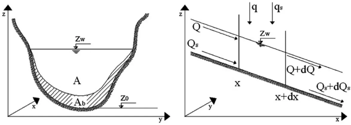
The model is based on a set of three differential equations, namely, the shallow water equations for dis-charge mass balance (see equation (4a)), the momentum balance (see equation (4b)) of the liquid phase, and the Exner equation for the mass balance of the solid phase (see equation (4c))
@A @t1 @Q @x5q; (4a) @Q @x1 @ @x Q2 A1gI1 ! " 5@I1 @x jzw2gASf; (4b) 12p ð Þ@A@tb1@Qs @x 5qs: (4c)
Here t is the time, x is the longitudinal stream coordinate, A is the cross-section wetted area, Q is the liquid discharge, g is the gravity acceleration, I1is the static moment of the wetted area A with respect to the
water surface, Sfis the friction slope, Abis the sediment volume per unit length of the stream subject to
ero-sion or deposition (sediment area), Qsis the solid discharge, q and qsare the liquid and solid lateral inflows
(or outflows) per unit length, respectively (see Figure 4).
The first term in the right-hand side of equation (4b) represents the variation of the static moment I1along
the x coordinate at a constant water level zw[Capart et al., 2003; Schippa and Pavan, 2008]. This formulation
avoids an undesirable explicit definition of the local bed slope in the momentum balance equation that often leads to incorrect momentum balance in natural rivers.
To complete the equations system, two closure equations have been used, i.e., Manning formula [Manning, 1891] for computing the friction slope, and Engelund-Hansen formula [Engelund and Hansen, 1967], for computing total sediment transport (bed load and suspended load together). The latter has been tested and compared to other sediment transport formulas during previous extensive studies on the Po river
Figure 3. The gray area is the feasible domain defined by equations (1) and (3), within which alternative operating rules can be designed. A specific rule (bold black line) is specified by instantiating the four parameters h1, h2, h3, and h4.
[Ministero delle Politiche Agricole Alimentari e Forestali, 1990], and was representing sediment movement in this reach well.
As for the sediment mass balance, the solution of equation (4c) updates the value of Abat every time step.
For every wetted point of the cross section, the variation of this value has to be converted into an elevation difference, Ds. It is assumed that Ds is proportional to bed shear stress, and consequently to local water depth h through a constant k:
Ds5kh: (5)
The variation of sediment area DAb, at every time step, is obtained by integration of Ds along the wetted
perimeter P
ð
PDs dp5DAb
: (6)
The same integration on the right-hand side of equation (5) leads to the wetted area A. Therefore, k is known and the local bed variation due to erosion or deposition is computed directly via equation (5). To integrate equation (4), the finite difference explicit scheme developed by McCormack was chosen, for its easy implementation and its ability to cope with discontinuities in the solution.
The river stretch is split in two substretches: the first is from Piacenza to IS dam (30 km) and the second from IS dam to Boretto (82 km) (Figure 1). In a field campaign in 2009, the Interregional Po Agency (AIPO) surveyed 67 cross sections in the two substretches, with an average spacing of 1.69 km. For every cross sec-tion survey, the boundary of the overbanks and the thalweg was identified. In the model simulasec-tions the interdistance between the cross sections is reduced. Therefore, additional cross sections are derived by lin-ear interpolation from measurements, to reach a distance of 450 m between cross sections. This increased the number of cross sections along the reach to 250. Roughness coefficients were calibrated during previ-ous studies [Schippa et al., 2006].
The hydrodynamic boundary conditions at Piacenza and Boretto (historical discharge data and the stage-discharge function) are extracted from regional environment agencies bulletins. Four tributaries join the river in stretch 2. The power station channel joins the river between the Adda river confluence and Cremona. When the HP plant is operating, the two stretches 1 and 2 are disconnected: for stretch 1, the downstream boundary condition is the imposed water level, whereas the operating rule of the gate provides the upstream boundary conditions for stretch 2, both in terms of liquid (w) and solid dis-charges Qstr2;up
s . Modeling the sediment transport in proximity of the barrage requires some
assump-tions. When the power station is operating and the gates are at least partially closed, Qstr2;up
s is calculated as follows: Qstr2;ups 5Qstr1;downs ' 0:7 ' ð w a Þ 1:7; (7) where Qstr1;down
s is the sediment discharge approaching IS.
The empirical reduction coefficient 0.7 is applied to take into account the fact that not all of the eleven gates are necessarily open when the HPP is operating, so part of the sediment is retained. Anyway, it should be noticed that when power station is operating, water velocity and transport capacity upstream of the bar-rage are small.
When the discharge is above the safety limit, instead, all the gates are fully open instead. No flow is diverted to the power plant channel (u 5 0) and the two reaches 1 and 2 are linked. With all gates open, we may assume that full continuity is satisfied also for sediment transport, since most part of the sediment moves by saltation-suspension and not by traction close to the bed [Ministero delle Politiche Agricole Alimentari e Forestali, 1990].
4. Defining the Objectives
Two conflicting objectives are considered: the hydropower revenue and the incision rate in the reach under study (white line in Figure 1).
The expected yearly hydropower revenue Jhp[e/year] is the cumulated value of daily revenue over the
eval-uated time horizon (of n days) divided by the number N of years in the same horizon; the daily revenue is the product of the daily hydropower energy production (Pt) by the time-varying energy unit price pt(e/kW),
i.e., Jhp51 N Xn t51 ptPt; (8)
where n is the number of days and N the number of years in the evaluation horizon.
The hydropower production Pt(kW) is a function of the turbined release ut, the head jump Ht, and the
tur-bine efficiency g(Ht), which in turn depends on the head jump. That is,
Pt5u g q gtutHt; (9)
where u is a coefficient for dimensional conversion, g is the gravitational acceleration (9.81 m/s2), and q is
the water density (1000 kg/m3).
The hydraulic head is the difference between the water level upstream the gate (hupt ) and the water level
just downstream the turbines (hdown
t ):
Ht5hupt 2hdownt : (10)
Since the flow profile in the power station channel is not computed by the hydro-morphological model, hdownis assumed to be given by an empirical relationship: hdown5f(u, hjunc), where hjuncis the water level at
the junction between the power plant channel and the River Po, which is computed by the hydro-morphological model.
To quantify erosion we monitor the evolution of the bed level at five prespecified points within each cross section. The first point is the thalweg, and two other points are selected on the left and on the right side of the bed in each of M cross sections. Let us denote with zb
ijðyÞ the bed level in the ith point
(i 5 1,. . .,5) of the jth cross section (j 5 1,. . .,M) at the first day of the yth year of the evaluation horizon. The bed level change iyin the reach under study at the beginning of the yth year is defined as the
aver-age difference of level between the starting of the evaluation horizon and that instant all over the sampled points, i.e.,
iy55M1 X5 i51 XM j51 ðzbijðyÞ2zbijð0ÞÞ: (11)
To quantify incision resulting from any operating rule we consider the expected yearly incision rate over the evaluation horizon, i.e., we adopt as incision indicator Jinc(m/yr) such that
Jinc5i
N=N; (12)
A negative Jincindicates degradation. All variables needed for the calculation of the two objectives result
from the hydro-morphological model. Both the objectives, Jhpand Jinchave to be maximized.
5. Problem Formulation and Solution Procedure
The MO design problem for IS can thus be formulated min h J x h21 0 ;uh210 ;ah1 $ % ; (13a) subject to xt115ftðxt;ut;at11Þ t50; 1; . . . ; h21; (13b) ut5mtðat; hÞ t50; 1; . . . ; h; (13c) h2 H; (13d) ah
1given inflow scenario; (13e)
x05x0: (13f)
atis the incoming flow, utis the flow diverted to the HPP, and wtis the discharge that flows to the meander
through the gates of the barrage (see Figure 1). The flow utis led back into the main channel few kilometers
downstream. This is an established formulation for MO problems in water resources [Soncini-Sessa et al., 2007]. The target is to identify optimal operating rules m(%) that determine the diverted flow utas a function
of the incoming flow atand the design parameter vector h. The operating rules must be pareto-optimal in
the sense that they maximize the management objectives Jhpand Jinc. The hydro-morphological model
component is represented in the control law by xt115ftðxt;ut;at11Þ. It is a lumped spatially distributed
dynamic model capable of producing the necessary information related to water and riverbed levels (the vector of states x) to calculate the objective vectors J. The objectives for this case study Jinc xh21
0 ;uh210 ;ah1
$ %, Jhp xh21
0 ;uh210 ;ah1
$ %
condense the information provided by the hydro-morphological model via time and space aggregation, in correspondence of a given evaluation inflow scenario (ah
1) [Soncini-Sessa et al., 2007].
The solution of Problem (13) requires thousands of evaluation of the hydro-morphological model. Ten years of simulation of the analyzed river stretch is run in approximately 1 day in a 3.4 GHz quad-core desktop computer. This makes direct computation of the objectives computationally demanding and hardly solvable within useful computational time. Hence, surrogate modeling techniques can be used to reduce the com-putational burden. In the following section we introduce the response surface methodology that was selected as a surrogate model in this case study.
5.1. Response Surface Methodology
A wide variety of surrogate models have been developed over the past decades and their use is becoming more and more popular within the water resources community [Razavi et al., 2012]. The Response Surface Methodology (RSM) was first proposed by Box and Wilson [1951] and was widely implemented both for single-objective and MO optimization [Kleijnen, 2008].
In this case study we adopt the Learning and Planning RS (LP-RS) procedure proposed by [Castelletti et al., 2010a], to solve the MO design problem using a global interactive response surface methodology. Technical introductions to this method can be found in Castelletti et al. [2010a] and reference therein. Here we pro-vide some basic principles of the LP-RS procedure. Appendix A introduces some more technical details in order to support future applications.
A classical optimization algorithm for solving the design problem (13) evolves in the space of the design parameter vector h and evaluates the corresponding value of the objective J by simulating the system behavior under a given operation rule. The process ends when the minima of the objectives are found. As noted previously for our case study this approach would require thousands of simulations of the hydro-morphological model. Here is where a global GSM may be of help. Given the problem formulation (13), we are interested to understand the relationships between the objective J xh21
0 ;uh210 ;ah1
$ %
and the design parameter vector h. The function JðhÞ, linking objectives and possible operating rules, is named Response
Surface (RS). If the RS function was fully known a priori, it would be possible solve the problem (13) analyti-cally from
min
h2H JðhÞ: (14)
A complete direct determination of the RS surface is however computationally too expensive since it would require a high number of simulations of the model again. Thus an approximation ^JðhÞ of the RS is intro-duced using the LP-RS.
A certain number of appropriate instances of the operating rules (i.e., different values of the design parame-ter vector h) are chosen and the corresponding objective values J are deparame-termined via simulation of the hydro-morphological model: the number of instances is a trade-off between the need to properly cover the feasible set of the design parameter vector, and the concern of keeping the simulation time within accepta-ble limits. At the end of this simulation step, a first training set composed of (h, J) couples, is availaaccepta-ble and is used to identify a first approximation ^J1
ðhÞ of the Response Surface (RS) via interpolation. By assuming that the ^J1
ðhÞ properly represents the RS, the Design Problem 13 is substituted by the following: min
h2H
^ J1
ðhÞ; (15)
whose solution, the Pareto front in the space J, is straightforward. The solution of Problem 15 is the last step of the first iteration of the LP-RS procedure.
In order to check whether the approximation ^J1
ðhÞ of the RS is adequate, a few operating rules (i.e., a few values of the design parameter vector) are selected on the Pareto front and simulated via the PB model. These new simulations increase the number of couples (h, J) in the training set. With them an updated approximation ^J2
ðhÞ of the RS is identified and substituted instead ofJ^1
ðhÞ in Problem 15. The new Problem is solved and an updated Pareto front is obtained. This concludes the second iteration of the procedure. As in the second iteration, the third one also starts by choosing few points on the new Pareto front.
After the second and each following iteration, a termination test is performed to determine when to stop the procedure. We based our criteria on the RS accuracy. It considers the distances !jbetween the values of
the jth objective obtained via PB model simulation and the ones given by the RS approximation at the pre-vious iteration. If the average distance "!j is below a given tolerance kj, the Pareto front based on the
approximated RS is considered a good approximation of the PB model itself, and the procedure is termi-nated. Otherwise, a further iteration is performed. The thresholds kjhave to be set by the designer [Wang
et al., 2001]: their values are chosen according to the type of problem and the adopted objectives. Once more, the goal is to find the right compromise between the desired accuracy, and the available computa-tional power. In our case, the termination test verifies that the average distance "!jis only a small part of the
range Rjwithin which each objective Jj, computed by the RS approximation, can fall. Namely, the threshold
kjis the 6% of the difference between the maximum and minimum value assumed by the jth objective in the current LP-RS iteration. This means that we assume values of the approximated RS satisfactory as soon as their maximum error is negligible (less than 6%) compare to the range of objective values investigated.
6. Scheme A: Feedforward Control
6.1. Implementation
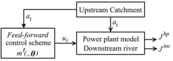
We consider first a pure feedforward control scheme (Figure 5), i.e., an anticipative control law. From a man-agement perspective, this means that at each time t the flow rate atentering the reach under study is
meas-ured and a release decision utis determined according to the operating rule mf(%) which is defined by the
design parameter vector h 5 [h1, h2, h3, h4].
The downstream incision rate could be limited through two different mechanisms: the increase of the sedi-ment supply to the downstream reach, so enhancing sedisedi-ment connectivity through the barrage, or the increase in discharge and transport capacity to mobilize previously settled sediments. The former is obtained by increasing the number of complete gate openings during medium-high flow events (currently it happens only for flows above 4000 m3/s, see Figure 2), namely by decreasing the threshold h
which the power plant is turned off. The lat-ter can be accomplished by diverting less water to the power plant. This first scheme (Scheme A) affects both sediment supply and transport capacity.
We started by simulating 49 different instantiations of the vector h including the BAU alternative. This relatively high number of simulations was necessary to test the model performance for the case study and to understand the system behavior initially. The main results have been analyzed in Bernardi et al. [2013]. The approximation of the RS can be derived as a function ^J :R4! R2that describes the relation between the four elements of the vector h and the corresponding values of the two objectives vector Jhpand Jinc, then. Identifying the RS approximation is a traditional
model identification problem as such it is composed of model selection (fixing the class of the RS), cali-bration (estimation of the parameters), and model validation, reiterated at each iteration over the updated training set of (h, J) couples. We considered five different functional classes: Radial Basis Func-tions (RBF), Thin-Plate-Splines, Multiquadratic and Cubic and General Regression Neural Networks (GRNN). The model validation is performed with a cross-validation technique [Kohavi et al., 1995]. The training set, obtained via the model simulations, is first normalized and then randomly partitioned into a calibration set and a validation sample set. For each considered class, a RS approximation is identified and the validation mean squared error (MSE) is computed for the validation set. The random partitioning is repeated 10 times. A final MSE is derived as average MSE over the 10 individual validation sets. The function class with the lowest averaged mean squared error in validation is then chosen.
The best interpolators for Jincand Jhpare then used to build the first approximation of the two RS, which are
evaluated on a discretized approximation of the feasible continuous set H, defined by equation (3). The dis-cretization of a continuous multidimensional set can be performed in many ways. Here, we build a hyper-grid and sample each hyper-grid point as an element of the discretized set H. The hyperhyper-grid is made of four equally spaced single grids, one for each element of the parameter vector h. To some extent this method is similar to the latin hypercube sampling [Tang, 1993; Park, 1994]. However, the grid spacing and form is not defined by a statistical law, here. But, it is based upon physical considerations on the system (heuristic method). Table 1 shows the ranges of values for the four element of H, the associated step of discretization chosen, and the deriving cardinalities of each element. The cardinality of the discrete set H is the product of the cardinalities Ni of the discretized set of the four parameter of h and was found to be 68.593 (see
Table 1, the combinations that do not satisfy the physical constraints have been removed).
The Pareto dominant solutions are then identified amongst this 68.593 alternatives. Finally the selection of interesting operating rules on the Pareto front to be simulated in the next iteration is performed by an expert (based on visualization techniques, see Lotov et al. [2004]). The procedure is iterated until the termi-nation test is satisfied.
6.2. Results
In the first iteration the 49 couples (h, J) are used to identify the best RS interpolation ^J. The best perform-ance is given by the GRNN interpolator for Jhpand by the Multiquadratic RBF interpolator for Jinc. Therefore,
these two interpolators are adopted. On their basis the Pareto-efficient alternatives are then identified and 26 alternatives are identified to be Pareto dominant over 68.593 alternatives. In Figure 6, they are repre-sented by the black dots on the dashed black line (Pareto front). Note that both objectives have to be maximized.
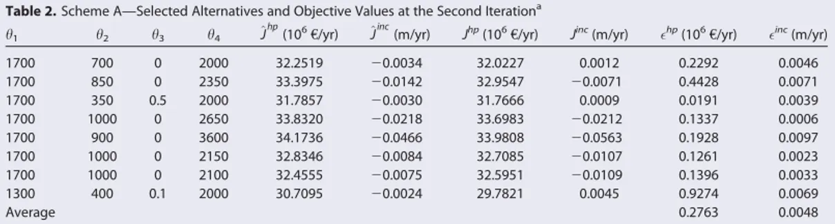
Interesting alternatives are chosen on the Pareto front, taking care of their physical meaning (the cor-responding operating rules). We selected eight interesting alternatives for simulation at the next iteration by the PB hydro-morphological model marked by the blue crosses in Figure 6. The values of the h elements and the associated objective
Figure 5. Scheme A— Feedforward control.
Table 1. Scheme A—Parameter Discretization
Parameter Range Step Ni
h1 900–1700 50 17
h2 200–1000 50 17
h3 0–1 0.1 11
values are in Table 2. Red circle points in Figure 6 show the locations of the eight points after the simulation of the hydro-morphological model. The arrows connecting crosses and circles visualize the differences !j between the approximated objectives (^Jhp and ^Jinc) and the simulated ones (Jhp
and Jinc) for those eight alternatives. The eight simulations are added to the previous 49 simulations
and used to compute an updated RS approximation. At this second iteration the best fitting is obtained again by the GRNN for both Jhpand Jinc. These two functional classed are then adopted
and, among the 68.593 approximated points of the RS, 42 are identified as Pareto dominant (red line in Figure 6). The procedure stopped here at the second iteration since the termination test is satis-fied (see Table 3).
The yellow star plotted on Figure 6 represents the performance of the BAU alternative, i.e., the current oper-ating rule, with an expected hydropower revenue of 34.28 (106e) per year and an expected incision rate of
20.0628 m per year. Results coincide with previous studies and call for effective management strategies in the future [Schippa et al., 2006]. The trade-offs inferred from Pareto front indicate that there are several pos-sibilities to reduce the riverbed incision process in the reach considerably with a moderate loss in hydro-power revenue.
Both simulated and approximated results reveal a characteristic system response: riverbed evolution is very sensitive to changes of h4. The best performing alternatives (i.e., those with the best Jhp=Jinctrade-off) are
those implementing the current operating rule changing only h4 (see Table 2 for details). Conversely,
changes in h1, h2, and h3result in substantial reductions in hydropower revenue without significantly
affect-ing incision rate.
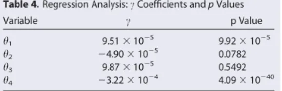
A regression analysis was performed to support these findings. A stepwise linear regression is derived from the 57 simulation results to infer the correlations between the components of the
Figure 6. Scheme A—Pareto fronts for first and second iteration. Blue crosses are the alternatives selected on the first Pareto front, red dots the values computed by the hydro-morphological model for those selected alternatives, and the yellow star is the BAU alternative.
Table 2. Scheme A—Selected Alternatives and Objective Values at the Second Iterationa
h1 h2 h3 h4 ^J
hp
(106e/yr) ^Jinc
(m/yr) Jhp(106e/yr) Jinc(m/yr) !hp(106e/yr) !inc(m/yr)
1700 700 0 2000 32.2519 20.0034 32.0227 0.0012 0.2292 0.0046 1700 850 0 2350 33.3975 20.0142 32.9547 20.0071 0.4428 0.0071 1700 350 0.5 2000 31.7857 20.0030 31.7666 0.0009 0.0191 0.0039 1700 1000 0 2650 33.8320 20.0218 33.6983 20.0212 0.1337 0.0006 1700 900 0 3600 34.1736 20.0466 33.9808 20.0563 0.1928 0.0097 1700 1000 0 2150 32.8346 20.0084 32.7085 20.0107 0.1261 0.0023 1700 1000 0 2100 32.4555 20.0075 32.5951 20.0109 0.1396 0.0033 1300 400 0.1 2000 30.7095 20.0024 29.7821 0.0045 0.9274 0.0069 Average 0.2763 0.0048 aBAU: h
design parameter vector h and the incision rate Jinc. Only the correlation between h
4and Jincis
statistically significant (see Table 4), which means that re-establishing hydraulic and sedi-ment connectivity during high flow events through a decrease in h4 appears to be very
effective in contrasting riverbed incision. Based on these evidences we propose a second scheme (Scheme B) where the value of h4 is fixed by a
feedback law: this is the subject of the next paragraph.
7. Scheme B
7.1. Implementation
Based on the results of Scheme A, Scheme B combines both feedforward and feedback control schemes (see Figure 7) together. The system is controlled by a feedforward operating rule as in Scheme A. But, at the end of each year y, a feedback operating rule mb(%) modifies the value of the parameter h
4of the
feedforward operating rule and the new value is maintained all over the following year on the base of the registered system output (more precisely the riverbed level variation iyregistered in the previous
year). The values of h1, h2, and h3are fixed to the BAU rule. Thus, the parameters of the feedforward rule
are all defined and the design parameter vector h is composed of the parameters that specify the feed-back rule only.
The aim of the control is to keep the yearly rate of riverbed level change iy=y close to a target value d (e.g.,
d 5 zero), i.e., to maintain a constant yearly rate of incision (or deposition). This means that the controller will determine a new value for the parameter h4based on the difference between the observed (iy) and the
target (dy) at the beginning of each year y of simulation. In mathematical terms, in the yth year the value of h4is given by
h45a1bðiy2dyÞ: (16)
Equation (16) is the feedback rule and a, b, and d are the three components of the design parameters vector. This means that the RS for ^Jincis a function of a, b, and d, which is the design parameter vector for Scheme B. Given a value of d, the alternatives we are interested in are those for which the feedback control law is effec-tive. That means it produces an average yearly incision rate Jincwhose value is d. These alternatives are
asso-ciated to the intersecting plane between the incision d and the surface ^Jinc in a 4-D space: an exemplification in a 3-D space is reported in Figure 8. Among the alternatives on the intersection plane, only those that maximize the hydropower revenue Jhpare Pareto dominant.
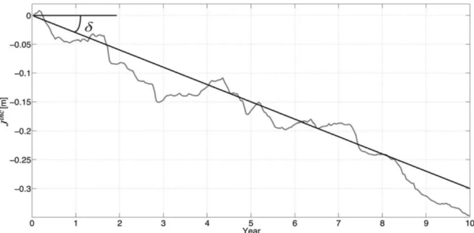
Scheme B was tested on few simulation runs in order to determine the most suitable range for each of the new components a, b, and d of the design parameter vector. As an example, Figure 9 reports the trajectory of incision (Jinc) obtained running the hydro-morphological model where h
4is produced by equation (16),
with a equal to 3700, b equal to 4000, and the targeted incision d equal to 20.03 (represented as a straight black line in the picture). The ranges of a, b, and d adopted and their discretization are presented in Table 5. The cardinality of the resulting discretized feasible set H is 22.997. On the base of these initial experiments, 25 simulations were used as a basis for starting the iteration cycle of the LP-RS procedure.
7.2. Results and Comparison With Scheme A
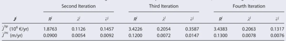
For Scheme B four iterations of the LP-RS procedure were necessary to satisfy the termination test (see Table 6), with a total of 58 simulation runs of the hydro-morphological model. Figure 10 shows the convergence of the Pareto front over the four performed iterations. The top graph of Figure 10 shows the progression from the first iteration Par-eto front (dashed black line) to the second itera-tion Pareto front (red line) along with the 11 selected alternatives (blue crosses) which were simulated (red circles) in order to obtain the
Table 4. Regression Analysis: c Coefficients and p Values Variable c p Value h1 9.51 3 1025 9.92 3 1025
h2 24.90 3 1025 0.0782
h3 9.87 3 1025 0.5492
h4 23.22 3 1024 4.09 3 10240
Table 3. Scheme A—Termination Test: The Average Distances "!j
Are Compared to the Thresholds kj(6% of the Ranges Rj)
Jj Rj kj "!j
^Jhp(106e/yr) 10.9529 0.6571 0.2763
second iteration front. Analogously the bottom graph in Figure 10 shows the pro-gression from the third to the fourth itera-tion front. Once again the arrows help visualizing the differences !j between the
approximated objectives (^Jhpand ^Jinc) and the simulated ones (Jhp and Jinc) for the
selected alternatives at each iteration. The termination criteria is satisfied at the fourth iteration thus terminating the pro-cedure (see Table 6).
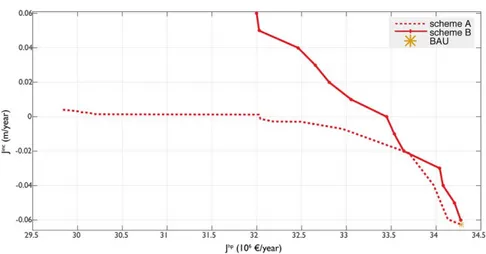
Figure 11 compares the Pareto fronts determined with Schemes A and B. It is apparent that Scheme B dominates Scheme A. In particular:
1. Stopping the incision would cost e 2.5 million per year due to the consequent reduction in the hydro-power revenue (about 7.3% of the current yearly production) when adopting Scheme A, but only e 0.8 million per year (about 2.6% of current yearly production) when adopting Scheme B.
2. Halving the current rate of incision in the reach downstream from Cremona would cost e 0.5 million per year (about 1.5% of current yearly production) with Scheme A and only e 0.2 million with Scheme B (0.6% of current yearly production).
In addition, Scheme A does not allow to achieve any aggradation in the riverbed in order to restore previ-ous degradation. This is possible with Scheme B: an aggradation of 2 cm/yr would cost e 1.6 million (about 5% of current yearly production).
Scheme B is conceptually more advanced than Scheme A. It provides an online control of the riverbed varia-tion. The performances of Scheme A depends on the hydrological series used to run the optimizavaria-tion. In a context of fast changing flood occurrences its operating rules may result not so effective. The feed-back control of Scheme B is more resilient with this respect since the operating rule adapts itself to the new dis-charge inputs every year.
8. Discussion
The RSM provided a flexible approach to solving the design problem. This paper showed the potential of RSM which was previously applied to integrate a number of complex processes into WRM [Castelletti et al., 2010a] to embed fluvial geomorphological processes into WRM. Hence, a topic is addressed, and solved
Figure 7. Scheme B—Mixed feedforward and feedback control.
Figure 8. Control of morphological evolution: actual (gray, curve line) and targeted (black, straight line) trajectories of the incision (experi-ment with a53700; b54000; d520:03 in equation (16)).
here from a quantitative WRM perspec-tive that was so far mainly acknowl-edged in qualitative terms [Petts and Gurnell, 2005].
The proposed case study of Isola Ser-afini is used as an illustrative example to introduce the general methodo-logical framework. The model is applicable to other case studies if a hydro-morphological model with mobile boundaries, i.e., capable of simulating channel adjustment proc-esses is available. This refers also to access to the detailed, morphologic data (cross sections) required for model setup. The subsequent implementation of the response-surface is, in contrast, readily feasible with standard tools.
To implement the framework on other real-word applications is necessary to strength our capacity to assess the uncertainty associated with the pareto-optimal solutions derived. There are a number of hypothesis in the current implementation of the method that are case study sensitive and should be carefully checked for real applications.
In terms of hydromorphological assumptions we assumed complete sediment connectivity when all gates are opened. This hypothesis produced results in line with previous works focusing on sediment transport and management scenarios on the River Po [Schippa et al., 2006]. For real application it should be supported by field evidences as this hypothesis is likely to change significantly in function of the dam infrastructures installed.
Regarding the RSM methodology specifically two parameters need to be carefully tuned: (i) the thresh-old for the termination test in the LP-RS procedure, (ii) the number of alternatives along the Pareto front selected for PB hydro-morphological simulations at each iteration. The number of selected alternatives to be simulated could be denser at neuralgic points where conflicts are more severe and hence of higher interest for management, for instance. At the moment, there is no established procedure to measure the quality of the Pareto front through the LP-RS procedure [Castelletti et al., 2012] since the full Pareto front is not known. In general, reaching higher accuracy would lead to higher computational costs, which would nevertheless still be lower than direct integration of a hydro-morphological model into the opti-mization process.
The resulting Pareto front is an effective tool to inform decision makers with quantitative data [Castelletti et al., 2007, 2010a, 2012]. Increasing or decreasing the hydropower plant production has a significant effect on riverbed evolution and the trade-off between the two issues is fully appreciable (see Figure 11). The pro-posed procedure provides valuable information to negotiate operating rules and subsidiary measures, which is nowadays a request of water resource related legislation, such as the European Water Framework Directive [EU Water Framework Directive, 2000], which establishes that a specific operating rule should be implemented only if countermeasures to tackle the degradation of the fluvial system are planned and undertaken.
In the case of IS scheme B could be easily implemented since it requires only to change yearly the discharge level at which all gates are fully opened for flood pass-through. A monitoring system could be set up on the river reach around Cremona to measure how the model prediction differ from the real channel process and if needed a re-calibration of the model could be undertaken supported by field evidences. If successful, the new operating rule will help stabilizing
Figure 9. An exemplification of the surface ^Jincin the 3-D space d, b, and Jinc. The
effec-tive alternaeffec-tives are the intersection points between the plane Jinc5 d and the ^Jinc
.
Table 5. Scheme B—Parameter Discretization
Parameter Range Step Ni
a 1200–4000 100 29
b 1000–7000 100 61
river infrastructures, limiting maintenance needs of navigation facilities and so counterbalancing the loss in hydropower revenue.
9. Conclusion
River geomorphology has become a key aspect of river management over the last years [Brierley et al., 2013]. However, the economical appraisal of direct and indirect ecosystem services affected by fluvial geomorphol-ogy is difficult to estimate [Newson and Large, 2006]. Fluvial geomorphic processes influence a variety of eco-system services like water supply (since groundwater levels can relate to riverbed level), freshwater ecoeco-system integrity and flood mitigation (by destabilizing river infrastructures and reshaping channel forms) [Ausseil et al., 2013]. For this reason the integration of river geomorphology into water resource management is receiv-ing growreceiv-ing attention [Yin et al., 2014; Wild and Loucks, 2014]. In this paper we provided a procedure to design optimal operating rules for a run-of-river power plant, which besides maximizing the energy production, reduce the riverbed incision rate downstream from the plant. To our knowledge, this is the first attempt to consider fluvial channel processes in designing operating rules from a MO perspective.
Table 6. Scheme B—Termination Test: The Average Distances "!jAre Compared to the Thresholds kj(6% of the Ranges Rj)
Second Iteration Third Iteration Fourth Iteration Jj Rj kj "!j Rj kj "!j Rj kj "!j
^Jhp(106e/yr) 1.8763 0.1126 0.1457 3.4226 0.2054 0.3587 3.4383 0.2063 0.1317
^Jinc(m/yr) 0.0900 0.0054 0.0092 0.1200 0.0072 0.0147 0.1300 0.0078 0.0076
Figure 10. Scheme B—Pareto fronts at first and second iteration on the top graph and third and fourth iteration on the bottom graph. Blue crosses are alternatives selected on the first Pareto front (top graph) and third Pareto front (bottom graph), red dots are the values computed by the hydro-morphological model for those selected alternatives, and the yellow star is the BAU alternative.
To achieve this aim, we propose a framework that adopts the RSM a surrogate modeling approach to include PB hydro-morphological modeling into an optimization procedure. Hence, this framework over-comes the high computational costs that so far hindered the integration of river morphology into WRM. We provided numerical proof that river morphologic processes and hydropower production are indeed in con-flict, but that the conflict can be mitigated with appropriate control strategies.
Nowadays, various models exist to reproduce river channel processes from reach to catchment scales [Bra-sington and Richards, 2007]. This paper shows some currently unexplored potentials of coupling these advances with state of art in surrogate modeling [Castelletti et al., 2012; Razavi et al., 2012] to integrate more effectively fluvial geomorphology understanding into water resources management: a necessity no longer negligible.
Appendix A: Learning and Planning Response Surface Procedure
The Learning and Planning RS (LP-RS) procedure is a version of the RSM proposed by Castelletti et al. [2010a] for solving the MO Design Problem using a Global Interactive Response Surface Method. It consists of four iterative steps plus an initialization (Design of Experiment (DOE)) and a termination test (see Figure 12) [Castelletti et al., 2010a, 2010b].
Figure 11. Comparison of Pareto fronts between Scheme A and Scheme B.
In the first step (see Figure 12), at the kth iteration (k 5 1, 2, . . .) of the procedure, Nksimulations of the PB
model (see equation (13b)) are run, in correspondence of Nkdifferent instantiations h1,., hNkof the
parame-ter h and, for each instantiation, say the jth one, the corresponding value JðhjÞ is computed.
In the second step, the Nkcouples (hj, JðhjÞ) are used to identify, via interpolation, an approximationJ^kð:Þ of
the (unknown) RS Jð:Þ.
In the third step, the following MO design problem, based on the approximated RS, is solved: min
h2H
^
JkðhÞ; (A1)
and its Pareto front determined. If the number of considered alternatives is relatively small, as in our case, the optimization can be performed exhaustively i.e., comparing each alternative with all the others to iden-tify the Pareto efficient ones.
In the fourth step, this Pareto front is analyzed and Nk11interesting points ^J1, . . . ,^JNk11 are selected. The
cor-responding points h1, . . . , hNk11 in the parameter space constitute the new sample of the parameter h that
will be simulated at Step 1 of the subsequent iteration.
The Initialization step (Design Of Experiments DOE) requires to choose the first N1instantiations h1; ::; hN1to
be simulated at the first iteration (k 5 1). The DOE must effectively sample the decision space and can be based either on statistical techniques [e.g., Kleijnen, 2008], and references therein] or on the basis of physical considerations and a priori knowledge [Castelletti et al., 2010a, 2010c]. Starting from the second iteration, the termination test is performed as described in the text.
References
Ausseil, A., J. R. Dymond, M. U. F. Kirschbaum, R. M. Andrew, and R. L. Parfitt (2013), Assessment of multiple ecosystem services in New Zealand at the catchment scale, Environ. Modell. Software, 43, 37–48, doi:10.1016/j.envsoft.2013.01.006.
Bernardi, D., S. Bizzi, S. Denaro, Q. Dinh, S. Pavan, L. Schippa, and R. Soncini-Sessa (2013), Integrating mobile bed numerical modelling into reservoir planning operations: The case study of the hydroelectric plant in Isola Serafini (Italy), in WIT Transactions on Ecology and the Environment, vol. 178, edited by C. A. Brebbia, 13 pp., WIT Press, Southampton, U. K., doi:10.2495/WS130061.
Bonomo, F., and C. Luisa (2011), La nuova conca di Isola Serafini, Cemento Calcestruzzo, 105–115, Novembre 2011, Edizione PEI, Parma. [Available at http://www.edizionipei.it/uscite_riviste-quarry_and_construction-novembre_2011.html.]
Box, G. E., and K. Wilson (1951), On the experimental attainment of optimum conditions, J. R. Stat. Soc., Ser. B, 13(1), 1–45.
Brasington, J., and K. Richards (2007), Reduced-complexity, physically-based geomorphological modelling for catchment and river man-agement, Geomorphology, 90(3–4), 171–177, doi:10.1016/j.geomorph.2006.10.028.
Brierley, G., K. Fryirs, C. Cullum, M. Tadaki, H. Q. Huang, and B. Blue (2013), Reading the landscape: Integrating the theory and practice of geomorphology to develop place-based understandings of river systems, Prog. Phys. Geogr., 37(5), 601–621, doi:10.1177/
0309133313490007.
Burke, M., K. Jorde, and J. M. Buffington (2009), Application of a hierarchical framework for assessing environmental impacts of dam operation: Changes in streamflow, bed mobility and recruitment of riparian trees in a western North American river, J. Environ. Manage., 90, suppl. 3, S224–S236.
Capart, H., T. Eldho, S. Huang, D. Young, and Y. Zech (2003), Treatment of natural geometry in finite volume river flow computations, J. Hydraul. Eng., 129(5), 385–393, doi:10.1061/(ASCE)0733–9429(2003)129:5(385).
Castelletti, A., F. Pianosi, and R. Soncini-Sessa (2007), Integration, participation and optimal control in water resources planning and management, Appl. Math. Comput., 206(1), 21–33, doi:10.1016/j.amc.2007.09.069.
Castelletti, A., F. Pianosi, R. Soncini-Sessa, and J. P. Antenucci (2010a), A multiobjective response surface approach for improved water quality planning in lakes and reservoirs, Water Resour. Res., 46, W06502, doi:10.1029/2009WR008389.
Castelletti, A., A. Lotov, and R. Soncini-Sessa (2010b), Visualization-based multi-objective improvement of environmental decision-making using linearization of response surfaces, Environ. Modell. Software, 25(12), 1552–1564.
Castelletti, A., S. Galelli, M. Restelli, and R. Soncini-Sessa (2010c), Tree-based reinforcement learning for optimal water reservoir operation, Water Resour. Res., 46, W09507, doi:10.1029/2009WR008898.
Castelletti, A., S. Galelli, M. Ratto, R. Soncini-Sessa, and P. Young (2012), A general framework for dynamic emulation modelling in environmental problems, Environ. Modell. Software, 34, 5–18, doi:10.1016/j.envsoft.2012.01.002.
Dittmann, R., F. Froehlich, R. Pohl, and M. Ostrowski (2009), Optimum multi-objective reservoir operation with emphasis on flood control and ecology, Nat. Hazards Earth Syst. Sci., 9(6), 1973–1980.
Engelund, F., and E. Hansen (1967), A Monograph on Sediment Transport in Alluvial Streams, Teknisk Forlag, Copenhagen.
EU Water Framework Directive (2000), Directive 2000/60/ec of the European Parliament and of the council: Establishing a framework for community action in the field of water policy, Off. J. Eur. Communities, L327, 1–71.
G!omez, C. M., C. D. P!erez-Blanco, and R. J. Batalla (2013), Tradeoffs in river restoration: Flushing flows vs. hydropower generation in the Lower Ebro River, Spain, J. Hydrol., 518, 130–139, doi:10.1016/j.jhydrol.2013.08.029.
Grant, G. E., J. C. Schmidt, and S. L. Lewis (2003), A geological framework for interpreting downstream effects of dams on rivers, in A Peculiar River, Water Sci. Appl., edited by J. E. O’Connor and G. E. Grant, pp. 209–226, AGU, Washington, D. C., doi:10.1029/007WS13. Gupta, H., S.-J. Kao, and M. Dai (2012), The role of mega dams in reducing sediment fluxes: A case study of large Asian rivers, J. Hydrol.,
464–465, 447–458.
Acknowledgments
The authors wish to thank Sara Pavan at AIPO (www.
agenziainterregionalepo.it, Interregional Agency for Po River Management) for the early development and setting of the numerical model. River Po cross sections surveys have been kindly provided by AIPO. Flow data about Po River daily average flow rates and stage-discharge rating curves at several stations are freely available on ARPA website (www.arpa.emr.it, Emilia Romagna Environment Protection Agency). The authors also thank Rafael Schmitt for his precious comments. Finally, we thank the unanimous reviewers of the paper which helped us to improve the quality of the paper with their relevant comments.
Kleijnen, J. P. (2008), Response surface methodology for constrained simulation optimization: An overview, Simul. Modell. Pract. Theory, 16(1), 50–64.
Kohavi, R., et al. (1995), A study of cross-validation and bootstrap for accuracy estimation and model selection, in Proceedings of the 14th International Joint Conference on Artificial Intelligence, vol. 14, pp. 1137–1145, Morgan Kaufmann, San Francisco, Calif.
Kondolf, G. M. (1997), Hungry water: Effects of dams and gravel mining on river channels, Environ. Manage., 21(4), 533–551. Langendoen, E. J., R. R. Wells, R. E. Thomas, A. Simon, and R. L. Bingner (2009), Modeling the evolution of incised streams III: Model
application, J. Hydraul. Eng., 135(6), 476–486.
Lotov, A. V., V. A. Bushenkov, and G. K. Kamenev (2004), Interactive Decision Maps: Approximation and Visualization of Pareto Frontier, vol. 89, Kluwer Acad., Boston, Mass.
Magilligan, F. J., and K. H. Nislow (2005), Changes in hydrologic regime by dams, Geomorphology, 71(1), 61–78. Manning, R. (1891), On the flow of water in open channels and pipes, Trans. Inst. Civ. Eng. Ireland, 20, 161–207.
Ministero delle Politiche Agricole Alimentari e Forestali (1990), Po Acquagricolturambiente: l’alveo e il delta, vol. 2, pp. 184–195, Il Mulino, Bologna.
Newson, M. D., and A. R. G. Large (2006), ‘‘Natural’’ rivers, ‘‘hydromorphological quality’’ and river restoration: A challenging new agenda for applied fluvial geomorphology, Earth Surf. Processes Landforms, 31, 1606–1624.
Nicklow, J., and L. Mays (2000), Optimization of multiple reservoir networks for sedimentation control, J. Hydraul. Eng., 126(4), 232–242, doi: 10.1061/(ASCE)0733–9429(2000)126:4(232).
Nicklow, J. W., and O. Ozkurt (2003), Control of channel bed morphology in large-scale river networks using a genetic algorithm, Water Resour. Manage., 17(2), 113–132.
Park, J.-S. (1994), Optimal latin-hypercube designs for computer experiments, J. Stat. Plann. Inference, 39(1), 95–111.
Petts, G. E., and A. M. Gurnell (2005), Dams and geomorphology: Research progress and future directions, Geomorphology, 71(1), 27–47. Poff, N. L., and D. D. Hart (2002), How dams vary and why it matters for the emerging science of dam removal, Bioscience, 52(8), 659–668,
doi:10.1641/0006-3568(2002)052[0659:HDVAWI]2.0.CO;2.
Razavi, S., B. A. Tolson, and D. H. Burn (2012), Review of surrogate modeling in water resources, Water Resour. Res., 48, W07401, doi: 10.1029/2011WR011527.
Rosatti, G., A. Armanini, V. Galletta, M. Vergnani, and F. Cerchia (2008), L’uso dei Pennelli per la Riduzione Della Barra Forzata in Prossimita del Punto di Inflessione tra due Curve Susseguenti: Uno Studio Numerico Relativo al po, pp. 151–151, Atti del convegno 318 Convegno Nazionale di Idraulica e Costruzioni Idrauliche, Perugia, 9–12 Settembre 2008.
Schippa, L., and S. Pavan (2008), Analytical treatment of source terms for complex channel geometry, J. Hydraul. Res., 46(2), 753–763, doi: 10.1080/00221686.2008.9521920.
Schippa, L., and S. Pavan (2009), Bed evolution numerical model for rapidly varying flow in natural streams, Comput. Geosci., 35(2), 390–402.
Schippa, L., S. Pavan, and S. Colonna (2006), River Po low water training. The importance of mathematical modelling to support designing activities, in River Flow 2006, vol. 2, edited by R. M. L. Ferreire, E. C. T. L. Alves, and J. G. A. B. Leal, pp. 1973–1983, London, U. K. Soncini-Sessa, R., E. Weber, and A. Castelletti (2007), Integrated and Participatory Water Resources Management: Theory, vol. 1, Elsevier Sci.,
Amsterdam, Netherlands.
Surian, N., and M. Rinaldi (2003), Morphological response to river engineering and management in alluvial channels in Italy, Geomorphology, 50(4), 307–326.
Tang, B. (1993), Orthogonal array-based latin hypercubes, J. Am. Stat. Assoc., 88(424), 1392–1397.
Wang, G. G., Z. Dong, and P. Aitchison (2001), Adaptive response surface method—A global optimization scheme for approximation-based design problems, Eng. Opt., 33(6), 707–734.
Wild, T. B., and D. P. Loucks (2014), Managing flow, sediment, and hydropower regimes in the Sre Pok, Se San, and Se Kong Rivers of the Mekong basin, Water Resour. Res., 50, 5141–5157, doi:10.1002/2014WR015457.
Wu, F.-C., and Y.-J. Chou (2004), Tradeoffs associated with sediment-maintenance flushing flows: A simulation approach to exploring non-inferior options, River Res. Appl., 20(5), 591–604, doi:10.1002/rra.783.
Yin, X., Z. Yang, W. Yang, Y. Zhao, and H. Chen (2009), Optimized reservoir operation to balance human and riverine ecosystem needs: Model development, and a case study for the Tanghe reservoir, Tang river basin, China, Hydrol. Processes, 24(4), 461–471, doi:10.1002/ hyp.7498.
Yin, X.-A., Z.-F. Yang, G. E. Petts, and G. M. Kondolf (2014), A reservoir operating method for riverine ecosystem protection, reservoir sedimentation control and water supply, J. Hydrol., 512, 379–387, doi:10.1016/j.jhydrol.2014.02.037.