Claudio Boido, Antonio Fasano
CAPM with Sentiment
(doi: 10.12831/82216)
Journal of Financial Management, Markets and Institutions (ISSN 2282-717X)
Fascicolo 2, luglio-dicembre 2015
Copyright c by Societ`a editrice il Mulino, Bologna. Tutti i diritti sono riservati. Per altre informazioni si veda https://www.rivisteweb.it
Licenza d’uso
L’articolo `e messo a disposizione dell’utente per uso esclusivamente privato e personale, senza scopo di lucro e senza fini direttamente o indirettamente commerciali. Salvo quanto espressamente previsto dalla
Claudio Boido
University of Siena and Rome LUISS
antonio Fasano
University of Salerno and Rome LUISS
Abstract
We analyse the relationship between large cap returns and sentiment indexes, using a Capital asset pricing model (Capm) framework. We try to provide a better explanation of asset prices and their deviations from standard theories by means of sentiment indicators, assuming the latter being measures of the very inclination to speculate. Therefore, when sentiment is high, investor demand for specula-tive investment is high; conversely when it is low, investor demand for speculaspecula-tive investments is low. Unlike other studies, based on proxies, we use the European Sentiment Indicator and its constituents, based on direct surveys, to assess business and consumer confidence.
Keywords: Investor Sentiment; Stock pricing; Financial anomalies; Behavioural Finance; Capm. JEL Codes: G02, G11, G12, G14.
Part I
1 Introduction
1Emotions and mood may affect investors’ perceptions and thereby their investment decisions which in some ways are often difficult to unravel. It is important to establish that the sentiment effect can explain some of the anomalies observed in the market. In this way it does not mean that all decisions are irrational, but in some situations, when people are anxious and nervous their decisions may be affected by irrational factors and cannot be explained by traditional economic models. It is accepted that it is correct to analyse investors’ sentiment, because it helps to shed light on biases in investor stock market forecast and to give us the opportunity to make a profit by examining those biases. Consumer confidence is an indicator which stimulates the thinking investors to Corresponding author: antonio Fasano, Dipartimento di Scienze Economiche e Statistiche (DISES), Università di
Salerno, via Giovanni paolo II, 132 - 84084, Fisciano (Sa), [email protected]
1 This working paper is the final result of a research study carried by two authors. We can attribute Part I to Claudio
react to possible «states of the world» (recession, expectation, and euphoria). In this research we study the relationship between returns on the Italian Stock Index regarding large and small caps quoted on Italian Stock Exchange and consumer indexes. Consumer confidence increases when economic conditions are good, so consumers and companies are stimulated into borrowing money. On the other hand economic uncertainty causes pessimism, which reduces the demand for goods and money.
as for sentiment indicators, we base the analysis on consumer and business surveys conducted in Italy by the National Bureau of Statistic, under EU guidelines. These surveys demonstrate (among other things) the economic expectations of households and firms, fur-thermore they show their willingness to spend in durable goods or to expand production and their perception about current and future employment levels (see Section 4.2 for details).
2 Rational, or Irrational Investor, That Is the Question?
In recent years it has become clear that it is possible to identify two different schools of thought, concerning the response of traders in terms of stock prices to breaking news. The first group advocates rational expectations and market efficiency (on the basis of financial market theory people choose how to invest), while the second school of thought claims that in some situations people behave irrationally (where investors buy and sell instinc-tively). Rational investors use instruments for an expected return and standard deviation, while normal investors are affected by cognitive biases and emotions, which may influence asset prices at least theoretically. Thaler (1999) has examined five points (volume, volatil-ity, dividends, equity premium puzzle, predictability) where the behaviour seems to be at odds with the theories. Rational investors state that they know when it is better to buy or to sell, while fund managers often turn over their portfolios during the year. In a rational world, prices change every time news breaks, while stock and bond prices change more frequently, because they are more volatile and so the price changes without any reference to its intrinsic value. If the markets are strongly efficient, all existing information is included in the stock price. While, it is possible to make a profit if the investor knows confidential information before the financial market does. In this context «normal» investor reactions could be different to what many «rational» analysts expected. In 2008 the last «real estate bubble» burst and provided evidence to support those academics and practitioners, who stated that it is not only economic factors that affect the market, but also, in particular, sentiment and irrational considerations. It’s intuitive to understand that this statement relies on the fact, that in a rational and efficient market (in Fama’s meaning) without «herding effects» (when the investors act together without planned direction), bubbles should not occur. market anomalies easily support the quality of the thesis of behavioural economics and it is obvious to assert, that economics and finance paradigms should be revised to insert irrational investor behaviour in investment courses at Universities and at Business Schools. Recently akerlof and Shiller (2010) stated: «To understand how economies work and how to manage them and prosper, we must pay attention to the thought patterns that animate people’s ideas and feelings, their animal spirit. We will never really understand important economic events unless we confront the fact that their causes are largely mental in nature».
It is clear that the animal spirit plays a fundamental role in trying to explain most market anomalies and this would reduce the importance of the modern portfolio theory. This could define investor sentiment as the inclination to speculate, so when sentiment is high, investor demand for speculative investment is high, conversely when it is low, investor demand for speculative investments is low. It is correct to assert that some stocks are more sensitive to speculative demand and those which are more difficult to value, tend to be the riskiest to arbitrage. Fisher and Statman (2000) analysed the moods of three groups of investors: large, medium, and small. They associate Wall Street strategists as a large; writers of investment newsletters as medium and individual investors as small. They assert that there is a strong relationship between the sentiment of individual investors and the writers of the newslet-ters, while the other relationship is weak. The correlation of 0.47 is statistically significant, whereas the changes in the sentiment of strategists are not related to changes in the senti-ment of individual investors and newsletters. It is interesting to note that a combination of the sentiment between the three groups and S&p500 index is high.
3 Recent Literature
The rational investor makes a decision according to the axioms of the expected utility theory and he makes unbiased forecasts about the future. Efficient market Hypothesis (EmH) is based on investors who are rational and their valuation of securities is made rationally. Normal investors are not rational and their trading is random and they do not have an effect on prices. Even if investors were irrational it would be the rational arbitrageurs who would eliminate any distortion of the market. at the end of the last century Tversky and Kahneman (1981) asserted that the perceived risk may be affected by the framing of the non-economic and non-statistical facts at hand. Shiller, 1980 has shown that stock market prices are more volatile than what efficient market theory af-firms. In fact a stock market crash would not be justifiable if the market price took into consideration all the available information. many authors (Bernard, 1992; Jegadeesh and Titman, 1993; Chan, Jegadeesh and Lakonishok, 1996; Fama and French, 1988; poterba and Summers, 1988; Kothari and Shanken, 1997; Lo and macKinlay, 1990) have written about under reaction and overreaction, that is how security prices underreact or overreact to news which reaches the stock market. Bernard reviewed some evidence on market efficiency in relation to accounting earnings. The average initial response to earnings announcements is an underreaction, while extreme stock price movements represent over reaction to earnings. The concentration of the abnormal return in relation to subsequent earnings announcements. Jegadeesh and Titman (1993) have affirmed that the strategies to buy stock winners and to sell losers performed better in the first year, but this result was not confirmed in the following year. Chan et al. (1996) examined the predictability
of future returns from past earning news. They showed that the market reacts only gradu-ally to new information. Fama and French (1988) examined autocorrelation of stock returns and for the 1926-1985 sample period large negative autocorrelations for return horizons beyond a year are consistent with the hypothesis that mean reverting prices are important in the variation of returns. poterba and Summers (1988) analysed transitory
components account for a large fraction of the variance in common stock return. They concluded that the transitory components in stock price account for more than half of the variance in monthly returns. Kothari and Shanken (1997) studied the evidence that stock returns are predictable. They evaluated the ability of book to market ratio to track time series variations in expected market index returns and compared its forecasting abil-ity to that of dividend yield. They noted that over the period 1926-1991 the book to market ratio is stronger over the full period while the dividend yields relation was more solid in the sub period 1941-1991.
Daniel, Hirshleifer and Subrahmanyam (1998) and Hong and Stein (1999) have found that models based on investor behaviour create over or under reaction due to the presence of noise traders who are overconfident or have biased self-attribution in evaluating their performance. The problem is also caused by the presence of different classes of investors, who give different importance to the news, watching the impact of the fundamentals on price or on price trends. Hong-Stein studied the behaviour of two different groups of investors «news watchers» and «momentum trader»: there is a tendency for asset prices to underreact to news in the short run and there is another tendency for prices to over-react to news in the long run. The news watchers forecast is conditioned by confidential news about future fundamentals without observing past or current prices. momentum traders follow the past price changes without observing future fundamentals.
Sentiment is an abstract concept and therefore today the market can be optimistic, pessimistic or neutral, but this does not mean that today’s sentiment will be the same for future months. It believes that it is quite simple to identify sentiment when people use a survey to ask them to think about the factors that could affect the investment environ-ment over the next six months or how they rate the performance of stock markets over the next six months.
Sometimes it is important to know if investors make a distinction between the future of the economy and stock markets. positive sentiment is higher where consumer confi-dence and investor sentiment is positive. The survey could be described as a good proxy to help you if the sentiment is high or low. Obviously it must observe if the different surveys, published by database providers, are useful in improving dynamic asset allocation decisions, because they help us to know the sentiment of the stock market. The situation assumes greater importance, during periods of high volatility, in order to avoid losses or to reduce portfolio risk. In recent years active managers looking to improving dynamic strategies use active alpha management; therefore also in this context behavioural finance shows that sentiment is useful in order to increase outperformance with alphas.
Kyle (1985) and Black (1986) have put the study of market or investor sentiment in their theories of the noise trader models. They suggest that some investors negotiate on noisy signals without any link to fundamental data and so market prices can devi-ate from the intrinsic value, thereby not respecting Fama’s efficient market hypothesis. Behavioural theory assumes that interplay between noise traders and arbitrageurs fixes the market price and this is the opposite of the efficient market theory that affirms the market price of an asset differs minimally from the present value of expected cash flows and the arbitrageurs absorb demand shocks and shifts in investor sentiment. Shleifer (2003) affirmed that the assumption of investor rationally is contradicted by
psychologi-cal and institutional evidence. Efficient market hypothesis states that securities prices must equal fundamental values. He illustrates a new theoretical approach extending the research to the behavioural finance. He cites two principal foundations of behavioural finance: limited arbitrage and investor sentiment. The latter involves investors’ choice which is driven by heuristic «representativeness» and «conservatism». Representative-ness is the tendency for people to view events as representative of some specific class and ignore the law of probability in the process. Besides investors are conservative and do not update their behaviour models in line with possible market changes. These drivers take in overreaction and under reaction of investors on stock markets. according to traders it is well known that the best time to buy is when individual investors are pessimistic and to sell when they are optimistic. It is correct to ask if uniformed investors, called noise traders, have influence on the prices of financial assets. Long, Shleifer, Summers and Waldmann (1989) have shown how traders acting on non fundamental information could affect prices in a systematic way, the changes and the volatility in stock prices are explained not only by fundamentals, but also by irrational «noise trading». They have attempted to verify or deny the existence of noise traders in the US market for closed end investment which invests in securities. The difference, between the net asset value (so called NaV) of funds and its market price, is called the discount. as this value has varied since the former authors wrote the article, the behaviour of discounts may therefore be governed by the sentiment of the noise traders and so closed end funds have become a good sector of the market where researchers try to find noise traders. In this way a trader acting on non-fundamental information could affect prices and so we can identify two different types of investors. The first ones are driven by fundamentals to select on the basis of price and the second ones trade on noise signals. Consequently noise traders cre-ate an additional source of risk which adds to price volatility. The relationship between discounts and sentiment has shown that: when noise traders are bullish discounts should decrease because the market price increases and the difference is reduced and vice versa. In these model groups the most fundamental prediction of the noise trader is that ir-rational investors select on the basis of a noisy signal called sentiment. This causes risk and therefore price volatility. In some cases it uses a survey on a randomly selected group of members of an association of investors to measure investor sentiment directly. The question concerns contexts in which investors think the stock market will be in sixth month - bullish or bearish. On the basis of the survey’s results investors understand the direction of the sentiment. G. Brown (1999) showed that individual investor sentiment is related to increased volatility in closed end investment. He affirmed that high levels of individual investor sentiment are associated with higher level of volatility The right form, in which sentiment influences returns or volatility, is not as clear as before. If noise traders are sensitive to sentiment changes, then sentiment variations should drive returns and volatility. We expect that the level of sentiment will influence earnings and volatility. Neal and Wheatley (1998), Wang (2001), Simon and Wiggins (2001) show that sentiment can predict returns and use the positions held by large traders in the futures markets, as a proxy for sentiment. They also discover that they are useful for predicting the future returns in the next period. Wang studied the sentiment indicator in futures market. He found that the sentiments of large speculators are a price continuation indicator, while
large hedger sentiment is a contrary indicator. Investors are advised to go short when hedgers are turning bullish and to go long when they are turning bearish. So investors make profit if they buy when large speculators are bullish and large hedgers are bearish and sell when large speculators are bearish and large hedgers are bullish.
In the past articles Brown and Cliff (2004), Qiu and Welch (2004), Shiller (2000) found some solutions for identifying and measuring investor sentiment: direct, indi-rect, meta.
The following meanings can be highlighted:
– Direct: based on surveys which directly evaluate market participants sentiment. – Indirect: based on financial data and require theoretical backgrounds. They include buy-sell in balance, put-call ratio, Barron’s confidence index.
meta measurements: they are hybrid versions on direct and indirect measures. an example is a composite index consisting of common components coming from several sentiment proxies (closed end fund, number of IpO’s, turnover ratio, dividend premium.
Direct sentiment measures are based on polling investors and so the expectations of the market participants can be measured directly. In this case, if you analyse the answers to the questionnaire, many possible sources of errors may be identified. The polling of investors suffers from deficiencies common to most survey based studies, which have problems related to inaccurate responses regarding business conditions, employment conditions and family income for the following six months.
To measure indirect sentiment financial variables are needed, which require a theory linked to sentiment. The weak point is the need to build this theory and its respective interpretation.
meta measurements include analysts’ opinion, columns, and online forums; therefore it is based on a mixture of opinions.
In this kind of research the greatest deficiency is the short sale restriction for retail investors in the equity market. In fact when the investor decides to express a negative sentiment he could sell stocks short or he does not buy stocks, but he has a short sell restriction, so he has a difficulty in expressing a negative sentiment. Investors can discover another problem of disentanglement, which is the act of segregating institutional trade from retail trade. Baker and Stein (2004) includes a trading volume as a measurement of liquidity and therefore as a measurement of investor sentiment. In fact they assert that investors reduce liquidity when they are pessimistic. Sometimes a leading independent provider of investment research, such as Investors Intelligence, obtains information from independent market newsletters and assesses each author’s opinion of the market. Each newsletter is classified as bullish, bearish, or neutral regarding their expectations for future markets. Das and Chen (2007) investigate a methodology for analysing messages on stock message boards driven by providers like Yahoo! Generally it’s common to use statistical and natural language processing techniques to obtain the emotive content of a bearish, bullish or neutral signal. a valid measurement of sentiment is based on open-ing long call and openopen-ing long put options purchased by clients. The ISEE Sentiment Index is calculated by the International Securities Exchange (ISE) and in particular they calculate the ratio as follows: (opening long calls/opening put)/100. a value above 100 implies bullish sentiment, while a value under 100 implies bearish sentiment. Baker and
Nofsinger (2002) and akhtari (2011) attribute that weather factors induce bad moods and alter investors’ risk attitude. In fact Kamstra, Kramer and Levi (2003) have shown that stock prices tend to decline when Seasonal affective Disorder (SaD) prevails. Returns are significantly lower when the length of the day is shorter. In the following research Kamstra, Kramer and Levi (2008) find that during the fall season, when daily equity returns are low, daily Government Bond returns are high, as they should be if indeed risk averse investors shun risky stock and favour safer alternatives. This phenomenon is quite well known, because it is assumed that it is related to changes in the amount of daylight and so the length of the day and temperature are the only significant factors related to SaD. more recently mark J. Kamstra and Levi (2015) show that, on annual cycle in U.S. Treasuries, variations in mean monthly return are over 80 b.p. This difference peaks in autumn and declines in spring. They find that this seasonal cycle in Treasury returns is significantly correlated with a proxy for time varying investor risk aversion linked to seasonal mood change. particularly the depression arises with seasonally lower daylights in fall and winter. Boido and Fasano (2005) showed that individual investors are affected by psychological factors and that returns are low on monday because they are inclined to sell stocks, while on Fridays investors prefer to buy stocks.(daylights saving effect). SaD is a cyclic illness with recurrent episodes of (fall/winter) depression alternating with periods (spring/summer) with a normal mood. Chan and Lakonishok (2004) confirmed the importance of sentiment investors and they affirm that value stocks outperform growth stocks, but the relationship has deteriorated because of the bubbles. During the technology bubble (2000) over optimism caused stock valuations in the technology in-dustries to deviate from their intrinsic values. Recently Baker and Wurgler (2006) have examined the impact of investor sentiment. It is possible to associate the concept of beta with sentiment. It is imagined, after the great crisis, investors continue to be pessimistic and expect the market as a whole to decrease by 15%. They would herd toward the market index by buying and selling individual assets until their prices decreased by 15%. Those assets relative to other assets in the market might be sold rendering their beta a downward bias. This kind of herding behaviour would induce the betas on the assets to converge toward the market beta.
Basu, Hung, Oomen and Stremme (2006) have shown that the addition of sentiment variables to business cycle indicators improves the performance of the active portfolio and these results are statistically significant. The strategies based on sentiment exploit an overreaction, which leads to active alpha strategies. Kim and Ha (2010) show, using a version of Fama-French-Carhart four factor model (i.e. market, size, book market value, momentum), that sentiment affects the stock price of companies with a small cap, a low price and low book market value. m. Baker and Wurgler (2006) have proposed a sentiment index based on the main principal component of the following proxies: closed end fund discount, share turnover, number of IpO, the average first day’s return of IpO, the equity share in new issues and dividend premium. The stocks, that are hardest to arbitrage, tend to be the most difficult to value. Extreme growth stocks seem to be prone to bubbles consistent with the observation they are more appealing to speculators and optimists and to arbitrage. If there is a large number of investors who perceive the value of the stock to be higher than the current stock price,
the sellers have low sentiment for the firms while the buyers have high sentiment. It can be seen that there are millions of investors who have different sentiment levels. The sentiment level is dynamic and it is changing. Investors may change their senti-ment over time-depending on macroeconomic conditions, specific expert firms and analyst views. Consumer confidence increases (decrease) when investors grow bullish (bearish) but these investors do not always increase their stock return when consumer confidence is low.
Lawrence, mcCabe and prakash (2007) have shown how a stock price changes by modifying the components of the existing dividend discount model with the investor sentiment as a component. In this context stock price is governed not only by firm fun-damentals, but also by investor sentiment. The authors specify that investor sentiment affects both the expected growth rate and the expected discount rate. It is possible to evaluate the future performance of the company by individual beliefs. The traditional form of Capm incorporates investor sentiment with a modified beta, bs, as a
func-tion of beta and investor sentiment. If sentiment is high the firm will be perceived as less risky and the value of modified beta will be lower, thus reducing expected return (vice versa). Given the modified beta bs, Capm expected return the sentiment can
be expressed:
𝔼rs = rF + βs𝔼(r
M − rF)
Investors who think about the relevant future performance of a company will wait for a higher growth rate than those who believe that the firm is a certain failure. The growth rate for the firm is modified from g (the growth rate in the simple Gordon and Shapiro
model) to gs, where gs is a function of growth rate g and investor sentiment.
For a company where the investor expected return is greater than the growth rate and constant growth, the modified Gordon equation for the stock price is:
For an investors with strong sentiment for a company’s future performance, the expected discount rate rs will be low, while the expected growth rate gs will be higher,
thus making the value of the stock higher (as perceived by the investor). Similarly, the considered value of the stock will be small for investor with low sentiment for a firm’s future outlook. When the market price is higher than what the low-sentiment investor expects it should be, he will sell the stock. When it is lower than what the high-sentiment investor realizes it should be, he will buy it.
Blanchard and Watson (1983), Tirole (1982), Hong and Stein (1999) have affirmed that stock markets are influenced by price bubbles when it is difficult to make a forecast on the fundamental value of stock even if investors are considered to be rational.
P
r gs d s
0= 1
-Part II
4 Empirical Analysis: A Sample Application
among the main hindrances to the efficient market hypothesis is the presence of psychological biases on behalf of market participants. This makes theoretical (expected) prices, derived by Capm models, inconsistent with actual observed prices and the market factor inadequate to explain the excess returns.
Insofar as this diversion can be ascribed to the market «sentiment», we can attempt to augment the standard model by means of this psychological factor. It is common to capture investor sentiment indirectly through a proxy and a number of alternatives used by the literature were presented in Section 3. In this study, instead, we used the survey data feeding the European Sentiment Index.
To measure how and if the sentiment factor affects stock returns, we will build a multivariate factor model, in a Capm-like fashion, where the ordinary market factor is coupled with a sentiment factor for better explanation of stock returns. We will test the model fitting with and without the behavioural factor and, as long as sample data is consistent with the theory exposed here, we expect to obtain a better fit in the latter case.
One problem we face in analysing return dynamic is given by the relatively large number of sample stock returns to be confronted with market and/or sentiment factor: in fact for some stocks, tests can confirm the theory behind the model; for others tests could be not meaningful or even contrast sharply with theoretical assumptions. We therefore need a robust method to aggregate single-stock behaviour into a market-wide dynamic. We discuss in deep the approach to address these questions, and the underlying assump-tions, in Section 5.
Before diving into the model technicalities, we will discuss the data set (Section 4.1), particularly the main data source of this study, the Joint Harmonised EU Programme of Business and Consumer Surveys, with the related sentiment indicators (Section 4.2).
4.1 Data Set
The data set, obtained via Bloomberg service and the EU public access data, is consti-tuted of time series concerning: the Italian FTSE-mIB index, FTSE-mIB constituents, Italian Sentiment Indicators and the Italian risk free rate proxied by means of Treasury-Bill gross rate2.
We use monthly log-returns spanning over the time window 1999-2011, including the sentiment index too, analytically treated as a price; for free rate, instead, we use Bloomberg calculated returns for free rate3 as is.
2 Italian T-Bills are named «Buoni Ordinari del Tesoro», BOT for short. We used the 3-month BOT gross rate time series calculated and published by Bloomberg platform on the basis of the related bond issues.
The Italian FTSE-mIB is constituted of the largest capitalisation stocks in Italy. Securities not available in the index as of January 1999 throughout to September 2011 were excluded.
The remaining 21 (out of 40) securities are shown in Table 1 along with their respective Bloomberg ticker.
4.2 Economic Sentiment Indicators in Europe and Italy
The European Economic Sentiment Indicators are produced by the European Commis-sion, through the Directorate-General for Economic and Financial affairs (DG ECFIN), in the context of the Joint Harmonised EU programme of Business and Consumer Sur-veys. These are qualitative economic surveys, intended for short-term economic analysis, which can offer signals for predicting turning points in the economic cycle.
The surveys are conducted on a monthly basis by means of questionnaires concern-ing five key areas4: industry, construction, consumers, retail trade and services. Nearly all
the questions are of a qualitative nature. These questions have a similar answer scheme, according to a three-option ordinal scale, that can be interpreted as a positive answer («increase», «more than sufficient», «too large», etc.), a neutral answer («remain unchanged», «sufficient», «adequate», etc.) and a negative answer («decrease», «not sufficient», «too small», etc.); but in some cases, respondents have the choice between more questions5.
4 Some questions are part of the questionnaire only once a quarter.
5 For instance, in the consumer survey respondents have a five-option ordinal scale. Table 1: The list of securities scrutinised included in the Italian FTSE-mIB
Company Bloom. Ticker
1 a2a Spa a2a
2 atlantia Spa aTL
3 autogrill Spa aGL
4 Banca pop Emilia BpE
5 Banca pop milano pmI
6 Buzzi Unicem Spa BZU
7 ENI Spa ENI
8 Fiat Spa F
9 Finmeccanica Spa FNC
10 Fondiaria-SaI FSa
11 Generali assic G
12 Impregilo IpG
13 Intesa Sanpaolo ISp
14 mediaset Spa mS
15 mediobanca mB
16 mediolanum Spa mED
17 pirelli & C. pC
18 SaIpEm Spa Spm
19 Stmicroelectroni STm
20 Telecom Italia S TIT
This scheme is intended to capture managers’ assessment of the trends in their sectors or households perceptions concerning the factors influencing their spending decisions.
Questionnaire data are mapped in five specific indicators, summarising judgements and attitudes of producers and consumers. Each indicator is based on a selection (not all) of the questions comprised in the questionnaire. For example the Industrial confidence indicator is built up upon the following three questions:
– Do you consider your current overall order books to be...? («more than sufficient», «sufficient», «not sufficient»)
– Do you consider your current stock of finished products to be...? («too large», «adequate», «too small»)
– How do you expect your production to develop over the next 3 months? It will... («increase», «remain unchanged», «decrease»)
as for the methodology, the indicators are built up upon the arithmetic average of the balances in percentage points of the answers to some (not all) of the questions deployed in the related area. Often balances are seasonally adjusted6.
a composite index, the Economic Sentiment Indicator (ESI), is derived by the five sectoral indicators applying to each a different weight.
Table 2 shows both sectoral indicators and their weight used in computing ESI. The surveys are carried out at national level by public and private partner institutes, selected by the Commission through a call for proposals every 3-4 years. The questions are harmonised following EU guidelines, however collaborating institutes at national level may include additional questions and the sectoral breakdown may be more detailed.
The EU Directorate General of Economic and Financial affairs is in charge to produce the aggregate surveys of the aggregate results received from the member States, based on weighted averages of the country-aggregate replies.
In Italy sentiment indicators are often referred to as «ISaE indices», since they were in charge of the Institute for Studies and Economic analyses (ISaE), however as from
6 For detailed methodology see European Commission - Directorate-General for Economic and Financial affairs (2007). Table 2: Sectoral indicators concurring to the definition of the Economic Sentiment Indicator (ESI)
Indicator Weight (%)
Industrial confidence indicator 40
Services confidence indicator 30
Consumer confidence indicator 20
Retail trade confidence indicator 5
Construction confidence indicator 5
Table 3: The family of EU indicators used in the analysis, based on Italian surveys conducted by the Italian National Bureau of Statistics
Confidence/Sentiment Indicator Industry (ITa) Services (ITa) Consumer (ITa) Retail (ITa) Construction (ITa) ESI (ITa)
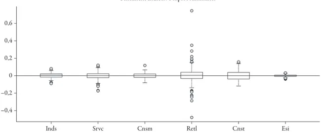
Figure 1: Box-and-whisker plots showing Tukey’s five number summary of the indices. 0,6 0,4 0,2 0 –0,2 –0,4
Inds Srvc Cnsm Retl Cnst Esi
0,043 0,15 0,4 0 –0,4 0,05 –0,10 0,05 –0,05 0,05 0,10 0 –0,15 –0,05
Correlations amog confidence indicators
Industry 0,29 0,22 0,072 Services 0,23 0,24 Consumer 0,059 0,11 Construction Retail 0,05 –0,05 –0,15 0 0,1 –0,05 0,05 –0,4 0 0,4 –0,1 0 0,1
Figure 2: Cross correlation among condence indicators. The upper triangle shows numerical values. To increase readability of the results, the more the correlation among styles the more the font dimen-sion. The inferior triangle shows the same data in the form of dispersion plots. The tted line for each
January 1, 2011 ISaE surveys and updates are part of ISTaT (Italian National Bureau of Statistics) surveys.
Our study is focused on Italian surveys and indicators as shown in Table 3. The time window spans from January 1999 to September 2011.
Some descriptive analysis concerning the indices follows.
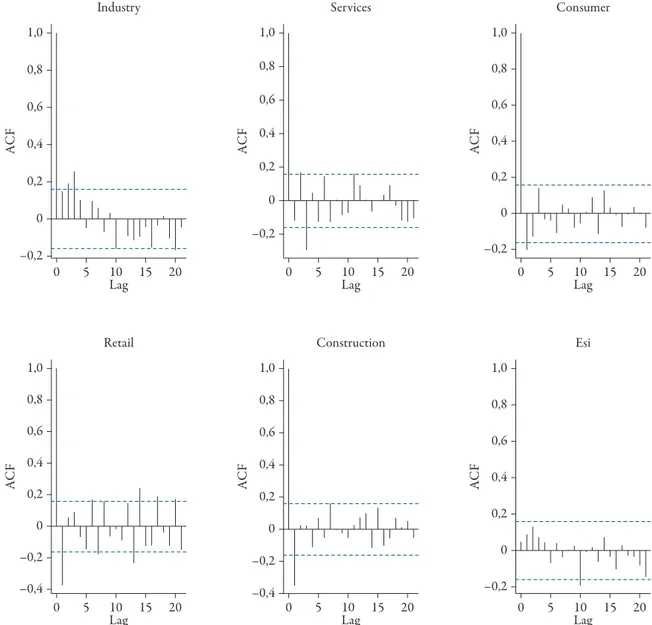
First, in Figure 1 Box-and-whisker plots show Tukey’s five number summary of the confidence indicators. Cross and serial correlations are then studied. In Figure 2 correlations among sentiment indices is shown. Figure 3 shows auto-correlation with different time lags for each index. as we can see, both cross and serial correlations are not significant.
Figure 3: Correlograms of each confidence indicator time series. The auto-correlations allow us to asses memory effects, that is the degree of correlation of present values of the series with past ones. The correlations are reported for different time lags and they can be considered negligible when contained between the horizontal bars.
1,0 0,8 0,6 0,4 0,2 0 –0,2 Lag AC F Industry 0 5 10 15 20 1,0 0,8 0,6 0,4 0,2 0 –0,2 Lag AC F Services 0 5 10 15 20 1,0 0,8 0,6 0,4 0,2 0 –0,2 Lag AC F Consumer 0 5 10 15 20 1,0 0,8 0,6 0,4 0,2 0 –0,4 –0,2 Lag AC F Retail 0 5 10 15 20 1,0 0,8 0,6 0,4 0,2 0 –0,4 –0,2 Lag AC F Construction 0 5 10 15 20 1,0 0,8 0,6 0,4 0,2 0 –0,2 Lag AC F Esi 0 5 10 15 20
5 A Factor Model to Explain Returns
as depicted in the introduction, we use a multivariate factor model to explain stock returns. The factors are the market and different sentiment indicators. Investor’s yield can be measured in term of excess returns as in Capm.
Before introducing the model, we set the notation and the variables that will be used throughout this paper.
Given a matrix A with dimension N × M, whose typical element is aij and enjoying
the property {(aij), it can be denoted with one of the following notations: ,
A a a a
N M# ij ijN M ij { ij ijN M
# , ^ h #
" , " ,
Similarly, the column-vector u and the row-vector v, with n components, could be
denoted with (omitting for short possible component properties):
u u v v n 1 i in n j j n 1 1 1 = = # # # # , " , " , The model variables are as follows:
1) rMt is the log-return of the market index at time t;
2) rit is the log-return of the i-th stock at time t, included in the market index;
3) rSt is the log-return of the sentiment index at time t;
4) rFt is the risk free rate at time t.
We denote with N the stock number and with T the number of observations, so that t = 1 ... T.
For each return, the equivalent excess return is defined as:
(1) r* r r
it= it- Ft
(2) rMt* = rMt- rFt
(3) r* r r
St = St- Ft
To help the vectoring of models we define also:
f1t = rMt f2t = rSt
The variables fkt* are defined by analogy with excess returns.
We can now model rit (and by analogy rit*) as a system of N × T equations:
(4) rit = ai+ b1i Mtr + b2i Str + eit (5) i .i f. K K t it 1 1 a b e = + + # # l where b.i= " ,bki kK 1# and f.i = " ,fkt kK 1#
The variables fkt play the role of common factors, that is observable regressor variables
which could explain the stock (excess) returns. In our analysis there are two common factors: the market factor and the sentiment factor; in spite of this, we find convenient denoting this number generically with K.
Note that, based on (4), we are assuming a constant intercept and slope in relation to time. In equations (4) stock returns are in scalar form. For a given stock i, the equations
(4) can be written in vector form as a system of N time series equations:
(6) y.i 1 y. 1 y. .
T 1 TT11 1i TM11 1i T S11 12i T i1
a b b f
= + + +
# # # # # # # #
Here y.i, y.M, y.S are the observed time series respectively of the i-th stock, the market
factor and the sentiment factor. We address the reader to appendix (a) for a more formal specification.
5.1 The Correlation Structure
Given the nature of the model, it is important to us the analysis of the correlation structure. To this end we find convenient to rewrite the model in a vectorised form. This entails: firstly stacking the equation in time series regression (6) as to obtain their matrix equivalent; secondly applying the «vec» operator.
(7) Y Z E
TN 1 TN N K 1N K 1 1 TN 1
C
= +
# # ^ + h ^ + h# #
While addressing the reader to appendix (a) for a formal discussion of the procedure, we observe here that Y is the vectorised return matrix, Γ is the vectorised coefficient
matrix (including the intercept) and Z is the vectorised factor matrix (augmented with
a proper 1-column vector). Clearly E is the error term for the model.
Given the vectorised-matrix model (7), the conditions concerning error term and factor correlations can be summarised as:
(8) Predeterminedness:E eh ti Zt = 0
N N K 1# + ` ^ ^ j h h (9) : 0, , Error correlations if otherwise e e t s E h t, h s j, ij 1 ! v = ^ ^ h ^ hh ) where eh(t, i) is the E element equivalent to eit.
We will now discuss these conditions and show the construction of matrix Zt.
By the very definition of «common factors» fkt, it seems reasonable to think that
they are uncorrelated with specific error terms. This assertion could possibly be false in some special case (i.e. for specific stocks with strong «systemic behaviour»), but it is supposedly true for the average stock. Formally this can be stated as:
If we look at (10) under another perspective, we can claim that factors have no power in explaining specific error terms. In place of the strong assumption of independence of residuals from past, present, and future factors’ values, we could limit independence only to current observations: this is to say that factors, as regressors, are predetermined (rather
than exogenous).
Eventually we replace (10) with the weaker condition:
(11) Predeterminedness:E r = E 0
r f it Mt St it kt kK 1 e e # = c ; Em ^ " , h
an important question is stock correlation. Of course disregarding stock correlation would allow us to deal with equations (6) individually. an independence (or null-correlation) assumption, while being easy for the calculations, appears too restrictive. The very fact that we take into account N equations/securities suggest that we need to take into account
how they interact with each other. Since we intend to focus on portfolios, we can choose to disregard serial in favour of cross-sectional correlation. This conveys to the condition:
(12) : , , Error correlations if otherwise t s 0 E it js ij ! e e v = ^ h )
Both conditions (11) and (12) are expressed with respect to the scalar model (4); they can be restated with regard to vectorised-matrix model (7), obtaining (8) and (9). We address the reader to appendix (B) for the formal derivation. Here we observe that Zt in (8) denotes the matrix obtained by stacking the N rows of Z containing
the t-th row of Z.
5.2 model Estimators
as showed in appendix (a), after proper transformations the N × T system of
equa-tions (4) is reduced to the linear model (7), with its related condiequa-tions for error terms. as a general rule, since this model appears to show both heteroscedasticity and se-rial correlations, a simple least square (OLS) would be inefficient. Based on this a GLS approach would be necessary, which in turn would require the knowledge of the error covariance matrix:
(13) X = cov(E) = 𝔼(EE´)
The GLS regressor for the model (7), based on (13) is: (14) C^GLS = (Z´X–1Z)–1 Z´X–1Y
On an empirical basis it could be anyway difficult to estimate (14), this would require some hypothesis concerning the error matrix, in fact Ω is (TN)2, which exceeds
as an alternative approach (to GLS), we use a heteroscedasticity-corrected covariance matrix or White adjusted. Standard errors for regression coefficients obtained are therefore
robust for non-constant variance7.
In order to implement the technique, we need to define a restriction matrix8.
Considering the vectorised coefficient matrix:
.1 .2 . N N N K 1 2 1 1 h a b a b a b C = # + ^ h R T S S S S S S S S SS V X W W W W W W W W WW
For each restriction to a given factor h we need to set bhi = 1 for all firms. Define C(h, j) as the vector obtained setting in C:
βki = 1 if k = h, i = j βki = 0 otherwise
It follows that, if we want to test the hypothesis of factor h coefficient being null, we set:
, , h h N 1 0 N N K N 1 g C C C = # + ^ ^ ^ h h h R T S S SS V X W W WW
5.3. Implementation
The empirical application was developed using the open source environment and language R. The code relevant to the scope of this paper is presented in appendix (C)
with detailed comments, to the benefit of other researchers interested to play with it. as detailed in the previous section, tests are implemented using a heteroscedasticity-corrected coefficient covariance matrix (so called «White-heteroscedasticity-corrected» matrix). The code is based on the R package «Car», maintained by John Fox and described in Fox and
Weisberg (2011).
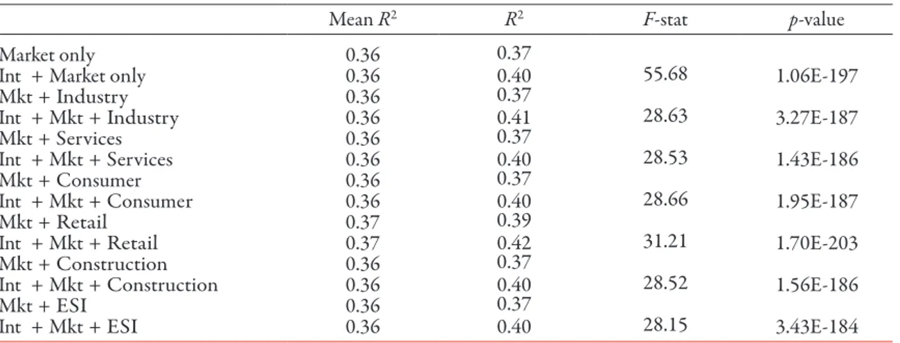
Table 4 shows the models obtained varying the sentiment indices, with and without intercepts. The single R-Squared for each model is presented connected to the
vector-ised multivariate model and the average of R-Squared’s of the sub-models obtained by 7 See White (1980).
8 In a restriction matrix (or hypothesis matrix) we have a row for each restriction applied to a coecient. Each row is constituted of ones in the positions of restricted coecient and zeros in the positions of unrestricted coecients. We also need the vector of restricted values, which is constituted of a scalar for each of those restrictions; the scalar value is the value which the coecient is constraint to. See e.g. Rencher (2003).
Table 4: Different sentiment models with fitting parameters, based on equation (7). Each model is obtained varying the sentiment factor and is fitted both with and without intercept. The single R-Squared for each model is presented connected to the vectorised multivariate model and
the average of R-Squared’s of the sub-models obtained by splitting the multivariate models into
a multiple regression for each security, as by equation (6). The fitting is based on White adjusted standard errors
mean R2 R2 F-stat p-value
market only 0.36 0.37
Int + market only 0.36 0.40 55.68 1.06E-197
mkt + Industry 0.36 0.37
Int + mkt + Industry 0.36 0.41 28.63 3.27E-187
mkt + Services 0.36 0.37
Int + mkt + Services 0.36 0.40 28.53 1.43E-186
mkt + Consumer 0.36 0.37
Int + mkt + Consumer 0.36 0.40 28.66 1.95E-187
mkt + Retail 0.37 0.39
Int + mkt + Retail 0.37 0.42 31.21 1.70E-203
mkt + Construction 0.36 0.37
Int + mkt + Construction 0.36 0.40 28.52 1.56E-186
mkt + ESI 0.36 0.37
Int + mkt + ESI 0.36 0.40 28.15 3.43E-184
Table 5: In order to measure the contribution of the sentiment factor to the models presented in Table 4, here the unrestricted version of these models (with the sentiment factor) are tested against restricted versions (without the sentiment factor). many sentiment indicators contribute to a better explanation of the returns; besides, consistent with Capm theory, lower p-values are obtained in the absence of the intercept
F-stat F p-value
mkt + Industry 2.70 4.55E-05
Int + mkt + Industry 1.72 2.12E-02
mkt + Services 1.20 2.38E-01
Int + mkt + Services 0.96 5.13E-01
mkt + Consumer 1.63 3.46E-02
Int + mkt + Consumer 0.40 9.93E-01
mkt + Retail 1.64 3.32E-02
Int + mkt + Retail 1.83 1.17E-02
mkt + Construction 0.81 7.16E-01
Int + mkt + Construction 0.82 6.93E-01
mkt + ESI 4.20 4.94E-10
Int + mkt + ESI 1.55 5.23E-02
splitting the multivariate models into a multiple regression for each security. There is a minimal difference between the two methods. Intercept models are also tested against the hypothesis of the factor coefficients being null (restriction matrix is built as detailed in Section 5.2). The p-values for these models appear highly significant.
The results in Table 4, while proving the effectiveness of the model, do not involve that there is an improvement or a significant contribution on behalf the sentiment factor. Therefore in Table 5 unrestricted models are tested against restricted versions without the sentiment factor (i.e. setting the sentiment coefficient as null) in order to check the contribution of psychological factors. It can be seen from the data here that many indi-ces show an acceptable degree of statistical significance (below 0.05), while the industry index and the general ESI provide a noteworthy contribution. most notably, as we can see from the table, the impact of the sentiment factors on returns is stronger when the test is run without the intercept, which proves coherent with the Capm model.
6 Conclusions
In this study, we analyse the impact of psychological biases on standard Capm models. If a market is dominated by crowd sentiment, then prices will not properly reflect stocks’ fundamentals therefore EmH assumptions are violated. Specifically, the market factor may be unable to fully explain stock excess returns, which may also be affected by market senti-ment. To address these issues, one might augment the standard model with this behavioural factor, trying to capture the role of noise traders into asset pricing equilibrium.
While the use of sentiment is not new in the context of asset pricing literature, numerous significant publications are based on proxy measures. a huge number of sentiment proxies have been proposed, but while indicators such as IpOs, dividend premia, etc. might give some insights on the prevailing market sentiment, they also expose the results to further biases due to researchers’ choice, which eventually lead to outputs inconsistent with one another and therefore likely to be proxy driven. as noted by Beer and Zouaoui (2013), despite the large number of proposals: «To date, the behavioural models are still silent as to what indicator should be used to assess their validity. Indeed, although numerous studies on the issue of investor sentiment have been published, little research has focused on their relative efficacy in predicting future stocks returns.» Direct measures are not immune from criticism mostly due to size and quality of survey samples, which tend to entail a specific (and often small) group of market investors.
Dissimilarly to other (proxied and direct) sentiment measures, the European Sentiment Indices are produced with direct data based on official surveys conducted in the context of the Joint Harmonised EU programme of Business and Consumer Surveys. These surveys are administered by national statistical bureaus respecting common standards in sample selections and, most of all, identifying different economic sectors resulting in the construc-tion of distinct sentiment indices. By using a multi-index approach, we are able to address the question of the relative efficacy of sentiment indices in predicting future stocks returns.
When comparing the explaining power of the standard Capm model with sentiment augmented models, the latter are able to give a better explanation of return dynamics, with respect to almost all of the sectors tested.
as testing different stocks can easily bear different and possibly conflicting results, in our empirical framework care has been taken in aggregating test results in the presence of heteroscedasticity, to avoid deriving meaningless conclusions with respect to the whole sample. The approach used is based on a heteroscedasticity-corrected covariance matrix (White adjusted). Besides, for each sentiment factor, the single R-Squared relative to the
vectorised multivariate model is compared to the average of the R-Squared’s of the
sub-models obtained by splitting the multivariate model into multiple regressions.
Our results show that the tting of the pooled regression does not equal the average fitting of the single regressions. In addition, the former can discriminate better among sentiment factors.
as our analysis is not aimed to the absolute fitting (which of course depends on the allocation efficiency of the market), but to test the improvement due to the behavioural component, we ran a battery of F-test to account for any economically significant
F-tests show that a significant contribution in explaining returns is given by
psycho-logical factors. Consistent with Capm theory, for almost all sentiment indicators, we obtain better results when the models do not include the intercept.
Summing up our analysis, based on blue chip markets, shows an improvement of the inference results if sentiment indicators are used. Several sub-indices connected with ESI show an improvement, and the best results are obtained with the main ESI index. Test-ing stocks of different kind and size – e.g. small or mid-caps, which are less correlated with overall market movements – might bring further insights on the sub ject matter.
Appendices
A. Vectorisation Procedure
We recall equation (6) for formal variable specification.
(15) y.i 1 y. 1 y. . T 1 TT11 1i TM11 1i T S11 12i T i1 a b b f = + + + # # # # # # # # (16) 1T X . T 11 1i T KK i1 T i1 a b f = + + # # # # # where: (17) y. y y r T t t t t T 1 1 = = # # K " K K K, with K = i M, or S (18) X x x f T K tk tk kt tk T K = = # # " , (19) e.i e e T ti ti it t T 1 1 f = = # # " , The model (4) can be written also in matrix form as:
(20) T NY 1T X B E T 11 N T K K N T N a = + + # # # # # # where: (21) N i i N 1 1 a= a # # " , (22) T NY# = "y yti ti= rit ti,T N# (23) B K N ki ki K N b = # # " , (24) T NE# = "e eti ti = fit ti,T N#
It could be noted that, based on (20), the typical element of the matrix Y is: (25) yti i xtk e k ki ti a b = +
/
+ (26) = ai + xt1b1i + xt2b2i + etiIf in (26) we substitute values from yti, xtk, eti based resp. on definitions (22), (18),
(24), we obtain:
rit = ai + f1tb1i + f2tb2i + eit
that is (4). It follows that (20) contains all the N × T equations (4) obtained by varying i, t.
Clearly estimating the matrix B and therefore its elements bki – by means of the
sin-gle matrix equation (20) – could bring results different by the individual estimates of the same parameters obtained, instead, by means of the single equations (4). The latter method could be potentially less efficient since two estimates b^ki, b^hj, despite individually optimal (that is with regard to the equations (4) whom they refer to), are not necessarily such contemporaneously.
It seems wise to operate on the (20) and, to this end, we vectorise it. So we set pre-liminarily: (27) T KZ 1 :T X T T K 1= 1 #^ + h 8 # # B (28) B K N N K N 1 1a C = # # # + ^ h > H
Therefore (20) can be written in matrix form as:
(29) T N T KY = Z 1 K C1 N T N+ E
# #^ + ^h + h# #
We now apply the «vec» operator:
(30) vecTNY IN Z vec vecE1
TN N K N K TN 1 1 1 1 7 C = + # # + + # # ^ ^ ^ h h h ABBBBC that is: (31) vecY vec Z Z Z E 1 .1 . . TN TN N K N N N K TN 1 1 2 2 1 1 1 f f h h h f h a b a b a b O O O O O O = + # # # # + + ^ ^ h h R T S S S S SS R T S S S S S S S S SS V X W W W W WW V X W W W W W W W W WW Eventually it can be worth rewrite (30) as:
(32) Y Z E
TN 1 TN N K 1N K 1 1 TN 1
C
= +
# # ^ + h ^ + h# #
where Y = vecY, Z = IN ∙ Z, Γ = vecΓ, E = vecE.
B. Correlation Structure in Vectorised-Matrix Form
We derive the correlation structure in vectorised form, i.e. with respect to (32). as for error correlations, given (12), the condition (12) can be easily reformulated in terms of (29) as: (33) 0, , if otherwise e e t s E it js E it js ij ! e e v = = ^ h ^ h )
In order to refactor (12) for model (32), we set:
(34) E vecE e e e , e TN TN h ti h t i i T t h TN 1 1 1 1 = = = = # # # - + ^ h ^ h " , Given (34), (33) becomes: (35) 0, , if otherwise e e e e t s E ti sj E h t i h s j, , ij ] v = = ^ h ^ ^ h ^ hh )
We now turn to predeterminedness. In order that we may express (11) in terms of (29), we set: (36) Z z z x z 1 T K tk tk tk tk tk T K 1 1 0 = = = # # + + ^ ^ h h " , Now, (11) becomes: (37) f e x e e z 1 0 E E E E it kt kK ti tk kK ti x ti tk kK 1 1 1 1 1 tk kK e = = = = # # # + # ^ ^ ` ^ ^ h h j h h 8 B " " " " , , , ,
as for the model (32), the Z regressor is a bit more cumbersome to work with. Looking
at the (31), we see that the Z matrix appears in N row of Z, so the t-th row of Z appears N
times in Z. We denote with Zt the matrix obtained by stacking the N rows of Z containing
the t-th row of Z (plus the adjacent zeros). The predeterminedness condition is therefore:
(38) E e zti tk kK E eh ti Zt 0 N N K 1 1 = = # # + ^ ` ^ ^ h h j h " ,
C. Main R Code
Due to space constraints, R code is omitted from printed article. It is available on request to interested readers.
References
akerlof, G.a. and Shiller, R.J. (2010). Animal Spirits: How Human Psychology Drives the Economy, and Why It Matters for Global Capitalism. Scottsdale arizona: princeton University press.
akhtari m. (2011) ‘Reassessment of the Weather Effect: Stock prices and Wall Street Weather’,
Undergraduate Economic Review, 7 (1), p. 19.
Baker H.K. and Nofsinger J.R. (2002) ‘psychological Biases of Investors’, Financial Services Review,
11 (2), pp. 97-116.
Baker, m. and Stein, J. C. (2004) ‘market Liquidity as a Sentiment Indicator’, Journal of Financial Markets, 7 (3), pp. 271-299.
Baker m. and Wurgler J. (2006) ‘Investor Sentiment and the Cross-Section of Stock Returns’, The Journal of Finance, 61 (4), pp. 1645-1680.
Basu D., Hung C.-H., Oomen R. and Stremme a. (2006) ‘When to pick the Losers: Do Sentiment Indicators Improve Dynamic asset allocation?’, EFa 2006 Zurich meetings paper.
Beer F. and Zouaoui m. (2013) ‘measuring Stock market Investor Sentiment’, Journal of Applied Business Research (JABR), 29 (1), pp. 51-68.
Bernard V.L. (1992) ‘Stock price Reactions to Earnings announcements: a Summary of Recent anomalous Evidence and possible Explanations’, Working paper University of michigan School of Business administration of Research n. 730.
Black F. (1986) ‘Noise’, The Journal of Finance, 41 (3), pp. 529-543.
Blanchard O.J. and Watson m.W. (1982) ‘Bubbles, Rational Expectations and Financial markets’, n. 945 National Bureau of Economic Research Cambridge, mass., USa.
Boido C. and Fasano a. (2005) ‘Calendar anomalies: Daylights Savings Effect’, The ICFAI Journal of Behavioral Finance, 2 (4), pp. 7-24.
Brown G.W. and Cliff m.T. (2004) ‘Investor Sentiment and the Near-Term Stock market’, Journal of Empirical Finance, 11 (1), pp. 1-27.
Brown G. (1999) ‘Volatility, Sentiment, and Noise Traders’, Financial Analysts Journal, 55 (2),
pp. 82-90.
Chan L.K., Jegadeesh N., and Lakonishok J. (1996) ‘momentum Strategies’, The Journal of Finance,
51 (5), pp. 1681-1713.
Chan L.K. and Lakonishok J. (2004) ‘Value and Growth Investing: Review and Update’, Financial Analysts Journal, 60 (1), pp. 71-86.
Daniel K.D., Hirshleifer D. and Subrahmanyam a. (1998) ‘Investor psychology and Security market Under- and Over-Reactions’, Journal of Finance, 53 (6), pp. 1839-1886.
Das S.R. and Chen m.Y. (2007) ‘Yahoo! For amazon: Sentiment Extraction from Small Talk on the Web’, Management Science, 53 (9), pp. 1375-1388.
European Commission - Directorate-General for Economic and Financial affairs (2007). Di-rectorate-General for Economic and Financial Affairs. The Joint Harmonised EU Programme of Business and Consumer Surveys. User Guide (updated 4 july 2007).
Fama E.F. and French K.R. (1988) ‘permanent and Temporary Components of Stock prices’, The Journal of Political Economy, 96 (2), pp. 246-273.
Fisher K.L. and Statman m. (2000) ‘Investor Sentiment and Stock Returns’, Financial Analysts Journal, 56(2), pp. 16-23.
Fox, J. and Weisberg, S.H.S. (2011). An R Companion to Applied Regression. London: Sage
publi-cations (second edition).
Hong H. and Stein J.C. (1999) ‘a Unified Theory of Underreaction, momentum Trading, and Overreaction in asset markets’, The Journal of Finance, 54 (6), pp. 2143-2184.
Jegadeesh N. and Titman S. (1993) ‘Returns to Buying Winners and Selling Losers: Implications for Stock market Efficiency’, The Journal of Finance, 48 (1), pp. 65-91.
Kamstra m.J., Kramer L.a. and Levi m.D. (2003) ‘Winter Blues: a Sad Stock market Cycle’,
Kamstra, m.J., Kramer, L.a., and Levi, m.D. (2007). Opposing Seasonalities in Treasury versus Equity Returns, Working paper available at SSRN 891215.
Kamstra m.J., Kramer L.a., and Levi m.D. (2015) ‘Seasonal Variation in Treasury Returns’, Critical Finance Review, 4 (1), pp. 45-115.
Kim T. and Ha a. (2010) ‘Investor Sentiment and market anomalies’, 23rd australasian Finance and Banking Conference.
Kothari S. and Shanken J. (1997) ‘Book-to-market, Dividend Yield, and Expected market Returns: a Time-Series analysis’, Journal of Financial Economics, 44 (2), pp. 169-203.
Kyle a.S. (1985) ‘Continuous auctions and Insider Trading’, Econometrica: Journal of the Econo-metric Society, pp. 1315-1335.
Lawrence E.R., mcCabe G., and prakash a.J. (2007) ‘answering Financial anomalies: Sentiment-Based Stock pricing’, The Journal of Behavioral Finance, 8 (3), pp. 161-171.
Lo a.W. and macKinlay a.C. (1990) ‘When are Contrarian profits Due to Stock market Over-reaction?’, Review of Financial Studies, 3 (2), pp. 175-205.
Long J., Shleifer a., Summers L.H. and Waldmann R.J. (1989) ‘The Size and Incidence of the Losses from Noise Trading’, The Journal of Finance, 44 (3), pp. 681-696.
Neal R. and Wheatley S.m. (1998) ‘Do measures of Investor Sentiment predict Returns?’, Journal of Financial and Quantitative Analysis, 33 (4), pp. 523-547.
poterba J.m. and Summers L.H. (1988) ‘mean Reversion in Stock prices: Evidence and Implica-tions’, Journal of Financial Economics, 22 (1), pp. 27-59.
Qiu L. and Welch I. (2004) ‘Investor Sentiment measures’, National Bureau of Economic Research. Rencher, a. (2003). Methods of Multivariate Analysis. New York (USa): Wiley, Wiley Series in
probability and Statistics.
Shiller R.J. (1980) ‘Do Stock prices move too much to Be Justified by Subsequent Changes in Dividends?’, National Bureau of Economic Research Cambridge, mass., USa.
Shiller, R.J. (2000). The Irrational Exuberance. princeton University press Wiley Online Library.
Shleifer, a. (2003). Inefficient Markets: An Introduction to Behavioral Finance. Oxford: OUp.
Simon D.p. and Wiggins R.a. (2001) ‘S&p Futures Returns and Contrary Sentiment Indicators’,
Journal of Futures Markets, 21 (5), pp. 447-462.
Thaler R.H. (1999) ‘The End of Behavioral Finance’, Financial Analysts Journal, 55 (6), pp. 12-17.
Tirole J. (1982) ‘On the possibility of Speculation under Rational Expectations’, Econometrica: Journal of the Econometric Society, pp. 1163-1181.
Tversky a., Kahneman D. et al. (1981) ‘The Framing of Decisions and the psychology of Choice’, Science, 211 (4481), pp. 453-458.
Wang C. (2001) ‘Investor Sentiment and Return predictability in agricultural Futures markets’,
Journal of Futures Markets, 21 (10), pp. 929-952.
White H. (1980) ‘a Heteroskedasticity-Consistent Covariance matrix Estimator and a Direct Test for Heteroskedasticity’, Econometrica: Journal of the Econometric Society, 48 (4), pp. 817-838.
Claudio Boido, Dipartimento di Studi aziendali e Giuridici (DISaG), Università di Siena, piazza S. Francesco 7/b, 53100 SIENa, [email protected]
antonio Fasano, Dipartimento di Scienze Economiche e Statistiche (DISES), Università di Sa-lerno, Via Giovanni paolo II 132, 84084 Fisciano (Sa), [email protected]