Analysis of moderate and intense rainfall rates continuously recorded over half a century and influence on microwave communications planning and rain-rate data acquisition

382

IEEE TRANSACTIONS ON COMMUNICATIONS, VOL. COM-35. NO. 4. APRIL 1987

Analysis

of Moderate and Intense Rainfall Rates

Continuously Recorded Over Half a Century

and -Influence on Microwave

Communications Planning

and Rain-Rate Data

Acquisition

AUGUST BURGUERO,

JOHN AUSTIN, ENRIC VILAR,

AND

MANUEL PUIGCERVER

Abstract-This paper is concerned with the statistical investigation of a massive data bank of 49 years of rainfall rate R continuously recorded in Barcelona using a rain-rate gauge with ten seconds response time. With radio communications in mind, the paper addresses and reviews in detail: 1) reliable statistical model for R , 2) number of years required to obtain a database from which to derive a reliable R-distribution, and 3) the CCIR worst-month concept.

The research has shown that the generalized Pareto a exp ( - p R ) / R b

gives nearly perfect fit for all ranges of R followed closely by the gamma distribution, and the simpler square root (R”*) normal distribution gives excellent fit too. The log-normal distribution was unsatisfactory for R 5

60 mm/h.

The spread of the yearly distribution of P ( R ) is cube root normally ‘distributed ( [ f ( R ) ] ” 3 ) and between 7 and 10 years are required before a reliable average distribution P(R) can he obtained. The study of the P ( R ) return time in years is also presented.

High resolution of P ( R ) is presented looking at the evolution of the annual P ( R ) in terms of the hourly and monthly contributing parts revealing statistical features such as the location in time of rain rates above 50 mm/h. Finally, the study shows that the calendar month contribution to P(R) remains at all times well below the synthetic CCIR worst month and recommendations are then given about its use.

I

I. INTRODUCTION

N recent years the increased congestion of the communications spectrum coupled with the requirement for greater bandwidth have brought about an increasing need for the use of the short centimeter and millimeter-wave parts of the spectrum in both terrestrial and satellite communication paths. Although the importance of rain as the main attenuation factor in the microwave radio links has been recognized for decades, it is more recently with the single- and dual-

polarization use of frequencies above 10 GHz, particularly for satellite communications, that the various aspects of the precipitation have been looked at in greater detail mainly by telecommunication administrations.

Although the specific attenuation y has been well estab-

Paper approved by the Editor for Computer-Aided Design of Communca- tion Systems of the IEEE Communications Society. Manuscript received September 5, 1985; revised July 12, 1986.

A. Burguefio and M. Puigcerver are with the Department of Atmospheric and Terrestrial Physics, University of Barcelona, Avenida Diagonal 647, Barcelona, Spain.

J. Austin and E. Vilar are with the Department of Electrical and Electronic Engineering, Microwave, Telecommunications and Signal Processing Re- search Group, Portsmouth Polytechnic, Portsmouth, PO1 3DJ United Kingdom.

IEEE Log Number 8613159.

lished to have the form aRb (e.g., [l]), where a and b are constants function of the frequency and R is the rainfall rate or intensity usually given in mm/h, the fact remains that R is itself a random process and therefore y is a random process too. In addition, to get the total attenuation, we will have to multiply y by an effective rain-cell length L ( R ) which is not

only a function of R but in general will be a function of the elevation of the path. To complicate matters, both R and L are functions of the climatic conditions of the radio link.

The climatic distribution of the rainfall intensity R has naturally attracted a great deal of attention-for instance, Crane [2] has proposed a global rain rate climatic division with 8 zones, combining the empirical approach of Rice and Holmberg [3] with climatological data, satellite cloud data, and microwave radiometeorlogical observations. This fol-

lowed earlier efforts of Dutton and Dougherty [4], [5] to produce detailed maps of precipitation rate R for Europe and the U.S.

When it comes to designing a radio link, or even to

contemplate the collection of data to study R , the fact still remains that R is a random variable and some basic questions remain, to a great extent, unanswered. They include for

instance:

1) the reliable statistical modeling of the distribution of R for all ranges of R ,

2) the number of years required to obtain a database from which to derive a reliable R distribution,

3) is the CCIR synthetic worst month a good safe margin or is it an over-design criterion,

4) what is the conditional distribution of R so that even after having exceeded a value R yet the duration

D

of the event lasts less than a specified lumber of seconds or minutes

D.

Questions l), 3), :!nd 4) have a direct impact in radio links whether terrestrial or satellite, where the attenuation and cross polarization are high if the intensity of rain is also high (ice depolarization apart). Also questions 3) and 4) are concerned directly with the over design or not of the communications system in terms of link availability.

This paper presents the analysis of a massive data bank of 49 years of continuous recording of R in Spanish Catalonia and addresses questions 1)-3). The rain gauge was of the Jardi- type and has about 10 s inherent time response (Appendix I).

Because of the high degree of statistical reliability answers have been found for the above questions. The subject of

question 4), intensity/duration, is currently under investiga- tion.

The material of the paper is covered in four sections. Section I1 describes the experimental procedures for the

BURCUENO et a/.: ANALYSIS OF MODERATE AND INTENSE RAINFALL RATES

generation of the data bank and in the Appendix, a brief description is given of the rain-gauge which appears not to be well known in literature of radio communications although it was designed back in 1921. Section 111 deals with the,annual distributions, the modeling, annual spread, confidencefmar- gin, and return time. Thus questions 1) and 2) are addressed in detail. Section IV deals with aspect 3) of monthly distributions whether real or synthetic (CCIR worst month). Finally,

Section V is concerned with additional information which was possible to derive from such large data bank, namely contours of R as a function of hour and month, etc. The study is mostly parametric but a great deal of effort has been put, whenever possible, to derive analytical expressions modeling the various results. Thus mathematical modeling of highly reliable statisti- cal results is also a key feature of this paper.

11. DATA BANK

A . Database

Since 1927 and even during the Spanish Civil War a Jardi rain-rate gauge has been in continuous operation in the Fabra Observatory at an altitude of 413 m in the Tibidabo Mountain of Barcelona. It is because of the mechanical simplicity of

operation of the gauge coupled with expectional careful

attention that a full set of chart recordings of the intensity R (mm/min) have been kept. The recordings investigated cover continuously 54 years from 1927 to 1981. They have been digitized at the University of Barcelona and the results

presented in this paper have been investigated jointly with Portsmouth Polytechnic at Portsmouth.

Each chart recording covers 24 h, has a length of 26 cm, and therefore 1 min is about 0.2 mm which in turn is about the resolution limit for manual digitization. The study has

revealed that it rained on average 1.2 1 percent of the time each year. Therefore the total number of hours of rain digitized was approximately 5724, equivalent to a length of 62

m

of chart recordings. Irrespective of the resolution and skill in the digitizing process, the authors have measured the step re-

sponse of the gauge which is 10 s (10-90 percent of the final value) and this gives confidence in the recording of very heavy rainfall of almost tropical nature which occur on the Catalo- nian coast (zone L CCIR [6]) with rapidly varying intensities and usually lasting only a few minutes.

The importance of the response time has been dealt with by several authors. Fig. 3 of [7] shows the impact using a fast response gauge of 10 s [8] as the integration time increases from 10 s to several minutes. Large rainfall rate events can be underestimated in their duration thus decreasing the cumula- tive probability P ( R ) = Prob ( R '

<

R ) : Clearly it is fortunate that the Jardi gauge had precisely about 10 s response time and thus the measured rates at Barcelona can be used with confidence. Similar impact of the response time of the

instrument on the statistics of R can be seen by inspection of Fig. 1 of [9] even though the times considered there were

longer and ranging from 5 to 60 min.

The lengthy digitizing process was carried out with great care by several students and researchers following as accu- rately as possible each one of the rain events. Computer

generation of the chart recordings and comparisons with the original chart recordings was carried on a few occasions to

check the digitizing process. The range 0-474 mm/h in the charts was covered in steps of 6 mm/h giving a total of 80 thresholds. The digitized values and the computed results

(inclusive of corrections due to curvature of the trace, real zero, invalid records or events, etc.) were saved in files. Additional values entered included the type of precipitation and a total of 3633 data files were finally generated. B. Generation of the Data Bank

As shown in Appendix I, the gauge should have. a linear response (displacement of a float) as a first approximation for

3.8 3

RAINFALL RATE (mrn/h)

Fig. 1. Experimental calibration (crosses) and modeling of the response curve of the Barcelona Jardi gauge.

100

1

_t

t

7. 7 6 -20 m

6

-40 rn -60 -80 Ln r. -100

1

1

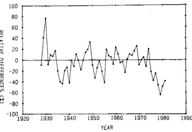
1920 1930 1940 1950 1960 1970 1980 1990 YEAR

Fig. 2. Relative error between Jardi annual integration height and direct height.

moderate R , and this was confirmed during detailed experif mental calibration. On the other hand the integrated value of the Jardi gauge over each year should agree within a reasonable margin of error with the annual rainfall amount recorded using conventional, techniques. T o convert the mechanical response to real precipitation rate R , the linear response was considered correct up to an R of 73 mm/h and the region beyond that was then approximated by a polynomial response. The experimental and best fit calibration curves are shown. in Fig. 1. This calibration curve with the particular break point at 73 mm/h' was selected as the one which

minimizes the difference between the annual amount directly measured by other instruments at the Observatory and the Jardi gauge. Fig. 2 shows the relative differences. The year 1930 was discarded as the difference is 77 percent. Also, 1978-1981 were rejected because the differences showed a trend to increase coinciding with the change in caretaker.

'

Nevertheless, for completeness of the data bank, the cumula- tive distribution of these years is presented and included in Fig. 16. Thus, the final bank selected spans 49 years. One

should notice that this cross-checking between the total rainfall and the integration of R over the year is desirable and thus, although the shape of the distributions may be correct, the absolute numerical values can only be obtained in this way. One should also note that these differences are mostly due to

'

The period 1978-81 corresponds to the change of caretaker at the Observatory who worked continuously there for over 50 years ensuring careful attention to the instrument, the serial number one of Richard of Paris.

3 84

IEEE TRANSACTIONS ON COMMUNICATIONS. VOL. COM-35, NO. 4. APRIL 1987

the low R ’ s ( R

,<

50 mm/h) which contribute about 80 percent of the total annual rainfall.

The raw data can be arranged in several ways according to the type of study. The added periods of time that a given threshold R of intensity is equalled or exceeded, T ( R ) , were divided by the various periods considered D so that T ( R ) / D would give elementary probabilities P ( R ) . The elementary periods

D

considered were 1) month, 2) hour, and 3) hour month.

Z)

Monthly Basis: This is the most important as the CCIR recommends that annual distributions as well as the worst month are both generated from this base [17]. If T,.(R), i = 1, 2 * 12, are the minutes per month, i, that the threshold R has been either equalled or ‘exceeded, then we have the 80 elementary probabilities (threshold levels of R ) and associated

[

40320

44640 min min

(or 4

i =

1, 1760

3,

5 , 7 , ’ 8 ,

leap year)

10, i 12 =

2

D i =

43200 min i = 4 ,

6, 9,

11

In addition the yearly matrix of data of 80 rows and 12 columns is complemented with P13 where Tl3(R) is given by

the total time I z T,.(R) and where Dl3 is either 525 600 min of an ordinary year or 527 040 for a leap year. Thus P13(R) is the conventional cumulative probability that R can be either equalled or exceeded. Finally, and for a given year, the worst month distribution P I 4 as recommended in [17] is given as the envelope of worst monthly probabilities. This is done by taking.for each R T,,(R) = Max [ T,(R), i = 1, 2

. . .

121 and as Dl4 one takes the relevant month i which gave the longest T, selected. -In practice and for computer applications the data were arranged as 49 arrays of length 80 X 14.

Because of the large data bank for each R and year considerd, the data P ; ( R ) can be considered a sample value of the set of random variables [ Pi(R)]. Also for each i , the 80 random variables are the discrete version of the continuous cumulative distribution probability Probi ( R ’ 3 R ) = P i ( R ) . This is why in Section

111-B

we carry out a statistical analysis of the ensemble of P i ( R ) with particular emphasis on i = 13, the annual distribution.

2) and 3) Hourly and Monthly-Hourly Basis: With a large data bank it is possible to carry out a reliable study of the diurnal distribution of R across the 24 h period over the whole of the 49 years, case 2). or even go to a higher resolution and consider the daily contribution to P ( R ) for each calendar

month [case 3)]. The result of these studies are given in Section V and the relevant probabilities are calculated in the usual way as the ratio between duration of “events” and period of time considered. In order to avoid too many points per day, the 24 hours (GMT) were divided into 12 periods of 2 hours each. This was found to give sufficient resolution and increased the reliability over a single 1 h interval.

111. ANNUAL CUMULATIVE DISTRIBUTIONS

A . 49-Year Average and Mathematical Modeling The 49-year average cumulative distribution

P * 3 ( R ) =

_-

i.

P j 3 ( R )

’i

/49

\j= I

/

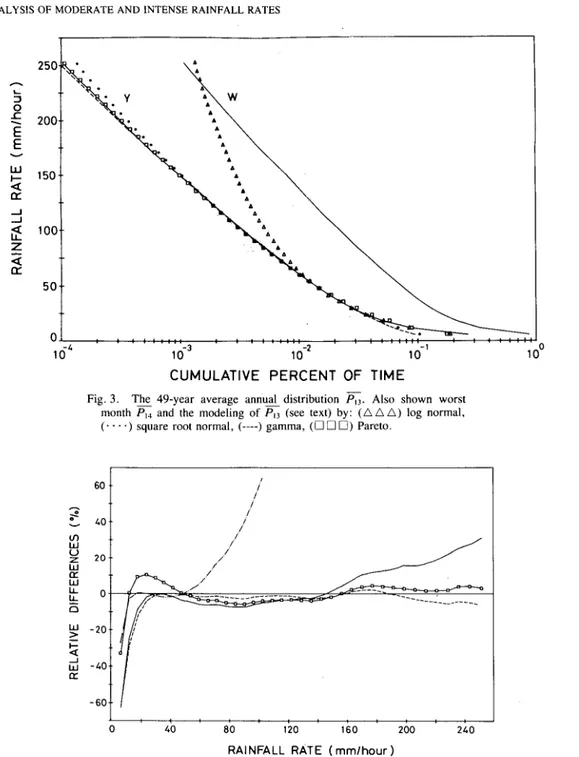
has been plotted in Fig. 3, together with theaverage worst month Pl4(R). Also shown is the modeling of P13 by the four

mathematical models discussed below. The annual average has been limited to lo-‘ percent, a value which corresponds to an accumulated duration of about 30 s in a year. Although the curve continues to increase monotonically well into where the plot begins to flatten due to lack of data, it was

thought more reliable to truncate P13(R) to Pl3(R)

<

percent.

average 1.2 1 percent of the time over the 49 year period. Thus to convert the annual statistics of the figure to, those under conditions of rain only, we must multiply the values by the factor 82.64 = 1/0.0121 (e.g., [18]). This value as well as other parameters which characterize the distribution would naturally vary with climatic and geographical locations.

The modeling of the distribution of R has attracted a great deal of attention in the past decade for obvious reasons of system planning. The literature survey points towards a general acceptance of the log-normal distribution, particularly in the U . S . Boithias, Lin, Fedi, and Segal among other investigators [ 181-1221 have considered this distribution in detail. The gamma distribution appears to be more accepted elsewhere particularly by Morita [23] in Japan in order to model all ranges of R , even though Boithias [18], the CCIR [24] and De Reffye [25] recommend its use only for relatively high intensities of about

R

>

50 mm/h. This is why De Reffye has proposed a generalized Pareto distribution which approxi- mates a log-normal distribution at low rates and a gamma distribution at high rates. This model would also include the power law proposed bySegal [22] for Canada.

In our investigation P13(R) was modeled with four theoreti- cal distributions: 1) log-normal, 2) square-root normal, 3) gamma, 4) generalized Pareto. The mathematical details and the numerical values of the parameters are given in Appendix 2. Fig. 4 shows the relative difference between the experimen- tal average and the models. We conclude from the study that the Pareto distribution models the experimental curve well for both high and low intensities followed closely by the gamma distribution. Fig. 2 of [18] gives, for several locations in Europe, a table of values of the two parameters of a gamma distribution. The system designer is thus faced .with the choice of either consulting the CCIR [24] and accept for his region the recommended values of R which can be exceeded for the quoted percent of the time (year), or select a particular mathematical model. To do this, he must select the associated parameters (whether two o r three) as well as find out the fraction of the time that it rains. If the mathematical modeling is the strategy selected, then in the ligkt of the results of Figs. 3 and 4 it appears that the root normal offers both good simplicity and fit. Nevertheless the Pareto distribution appears to be gaining acceptance [26], [27].

B. Spread of the Distributions-Modeling and Confidence Margins

Because of the large number of years available, we can follow the strategy of Moulsley and Vilar 1281 in the field of long-term scintillation statistics and group the yearly distribu- tions in independent sets of several years. The aim is to

observe the progressive clustering of the independent averages towards the final average of 49 years and thus obtain first a qualitative indication of the minimum number of years required for a reliable long-term distribution. Fig. 5(a) shows the family of 49 distributions. The averages are shown in Fig. 5(b)-(d) which contain, respectively, the average of 12 groups of 4 years each, 7 of 7 , and 4 of 10. The progressive clustering of each of the independent groups towards a final distribution is an indication of the existence of a characteristic distribution of the region. In fact, the average distribution of the first 25 years and that of the second group of 24 years are very close even though they cover ranges in excess of 300 mm/h and could be considered to represent periods about 1/4 of a century apart. We see that 7 years is the minimum period to get ‘a reliable statistic, but better estimations are obtained with an average of 10 years.

At this stage it is possible to give a numerical solution to this number of years required to get a reliable mean distribution.

-

BURGUERO el a / . : ANALYSIS OF MODERATE A N D INTENSE RAINFALL RATES

I

CUMULATIVE PERCENT OF TIME

Fig. 3. The 49-year average annual distribution

G.

Also shown worst month and the modeling of (see text) by: (AAA) log normal,

(. . . .) square root normal, (----) gamma, (00 0) Pareto.

:

1

oo

-

_P

e

6o 40

t

i i i I i

By grouping the years (49) in sets of

N

years we would get a family of means. This family of means, each of size

N,

constitute a population normally distributed. If we take the 5- 95 percent probability interval (90 percent confidence limits), then this interval spread is given by G ( R ) f u / f i x 1-64 where u is the standard deviation of the original population of P ( R ) ' s and P l , ( R ) represents the 49 years average curve. (One should note that for this study the 49 years average had to be assumed the best estimate of the mean.)

The dotted lines in Fig. 5(c) and (d) show the 49-year 5-95 percent confidence limits of the mean and it is clear that whereas most of the 7-year averages fall within that range, all the 10-year averages fall within the range. One should also note that this range gives confidence in using 7 (or 10) years in estimating the 49. We conclude that although 7 years is a

minimum, 10 is desirable. The possible dependence or not of

this criterion on climatic conditions and, hence, on the

structure of convective precipitation extends beyond the

intended scope of this analysis but the high degree of statistical reliability and independence of the group of observations

points definitely towards a safe range of at least 10 years. This is in agreement with earlier remarks on this subject [21].

A numerical indication of the spread of the 49 values o f P,@) for each R may be obtained from the standard deviation

u ( P 1 3 ( R ) ) . Thus the coefficient of variation or index of spread is given by

and is shown in Fig. 6.

IEEE TRANSACTIONS ON COMMUNICATlONS, VOL. COM-35, NO. 4, APRIL 1987

RATE

OF

RAINFALL (mmlhour) RATE OF RAINFALL (mmlhour)

BURCUEfiO et al.: ANALYSIS OF MODERATE AND INTENSE RAINFALL RATES

3 87

a v r. I d

d

25 50 75 100 125 150 175 200 225 250 2;s R A I N F A L L RATE ( m m / h )

Fig. 6 . Coefficient of variation of PI,(!?).

increase with R . It is linear in a logarithmic scale from about 12 mm/h where we get 35 percent and increases to 100 percent at 150 mm/h and to 200 percent at 250 mm/h.

The above study gives an indication of the magnitude in the spread of the values Pl3(R) (however reliable each one of the sample values might be). The question remains of the probability distribution or spread of these values. Are they normally distributed about some mean or are they mostly clustered around a median with tails in the distribution giving rise to the observed extreme distributions that one sees in Fig. 5(a). The study of the probability density (histogram) of values of P13(R) as

R

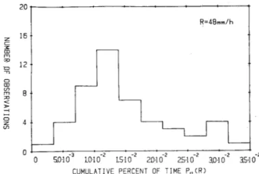
increases shows that for low R’s ( < 2 0 mm/h) the histogram has little skewness. However, for values of R 2 50 mm/h the skewness becomes very significant and therefore most of the 49 PI,@?) values are clustered around some median. This is naturally quite convenient particularly for high ,rates

R

and assists in the degree of reliability of PI3(R) for a given number of sample values. Fig. 7 shows a sample histogram for the case R = 48 mm/h. These histograms are obtained as we .observe the distributions of the Pl3(R) by “cutting horizontally” for each R in Fig. 5(a). The modeling of the distribution F, namely F(P13(R)) is important in order to give numerical values’of confidence in statistical terms. For example, we may wish to determine for each R , the fractional number (probability) of estimates of Pl3(R) which will fall within a specified range of the median PI3(R). For this, the F - distribution

was investigated in detail. The models considered were the gamma distribution, the log-normal distribution and the cube- root normal distribution all having a variable degree of skewness. The study was limited to R

<

160 mm/h. Up to about 100 mm/h the three distributions approximated the

family of histograms with a good fit. Above about 100 mm/h the log-normal distribution showed difficulty in following the experimental results. Finally, the cube root normal distribu- tion was selected and checked with a Kolmogorov-Smirnov test. This distribution can be written as

where for each R the random’variable X is in this case P , , ( R ) .

0

C U M U L A T I V E P E R C E N T OF T I M E P,,(R)

Fig. 7. Sample histogram of the spread of P,,(R)’s for R = 48 mm/h.

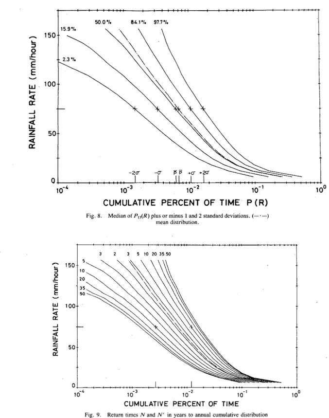
The distribution (4) has also been used by Segal [22] for similar purpose. Fig. 8 shows the mean distribution of the 49 years and then for each

R

we have plotted four selected values of the F distribution thus generating the continuous curves. They are the median and plus or minus one and two standard deviationcoy. One notices th$ because of the skewness, the average PI3 and the rned&Pl3 of this distribution do not coincide. In other words

=

PI^)"^

# ( P 1 3 ) ” 3 . This is seen clearly for the specific case marked in Fig. 8 of

R

= 75 mm/h. We see that on average this value will be exceeded 7 X

percent of the year. Nevertheless out of the cluster of, say, 49 values, 50 percent of these would be below about 6 X

percent and the other 50 percent would be above that value.

We can exploit further the distribution and again for R = 75 mm/h we see that (84.1 - 15.9) = 68.2 percent of the population P13 will have values ranging from 3.2 X to about 2 X percent. In other words, we can guarantee

with probability 0.682 that the values PI3(75) will be in that range. Something similar can be said for the range of spread

f 2 0 shown in the figure.

This interpretation of the F probability leads immediately and naturally to another interpretation, that of the return time which some readers may find more useful, although it is basically another way of looking at the spread of P13’s.

The return time is described and defined in the following way. Given a limit P ( R ) the question is how many years

N

are required so that among them one satisfies P,’,(R)

<

P I 3 ( R ) , and how many

N‘

are required so that one of them satisfies P,’,(R)

2

P W ) .

N

and

N ’

are then given by

and are known as return time (years) to a value smaller than X ( N ) or larger than X ( N ’ ) . Clearly only when the population of Pl3(R) has a symmetrical distribution we shall find

N

=:

N’.

Because we know that F ( X 1 i s skewed, therefore

N

=#:

N‘.

Fig. 9 shows the average PI3 and the associated return years. For example at R = 75 mm/h and out of 10 years of observation in the long run we shall find one with a Pl3(75) <: 2.6 X percent and one with a P I 3 ( 7 5 )

>

1.19 X lo-’ percent.

The solution between the probabilistic and return. time

interpretation of F[P13(R)] is clearly a matter of choice and omf physical insight into the spread of the population of annual cumulative values PI3(R).

3 8 8

IEEE TRANSACTIONS ON COMMUNICATIONS. VOL. COM-35. NO. 4. APRIL 1987

CUMULATIVE PERCENT

OF

TIME

P (R)

Fig. 8. Median of P,,(R) plus or minus 1 and 2 standard deviations. (-.-) mean distribution. * 3 2 3 5 10 20 35 50 5 10 20 35 50 150.- 100- - 50.- 0, c 1

o - ~

1 f 3 1

o-2

lo-' 1

oo

CUMULATIVE PERCENT OF TIME

Fig. 9. Return times N a n d N' in years to annual cumulative distribution values (see text). (-.-) mean distribution.

Iv.

MONTHLY DISTRIBUTIONS A N D W O R S T MONTH A . The Worst Month and Relation to the Annual

Distribution

The worst month cumulative distribution as recommended by the CCIR [17] was introduced earlier in the paper as array no. 14 of the P ; ( R ) ( i = 1 , 2

.

* * 14). The first 12 reflecting the monthly distribution. The average over the 49 years, P I 4 ( R ) was also plotted in Fig. 3 . This worst month distribution is defined in [17] as that month in a period of

twelve consecutive calendar months during which the selected threshold R is exceeded for the longest time. The selection of the longest time implies that if for a given year we had 12 monthly distributions, (our set P ; ( R ) i = 1 * *

.

12) we then select for each R the month which exhibits the highest P . The selection on a monthly basis of this highest P leads to a synthetic distribution which is an envelope of the monthly Pi's The necessity to account for extremes of probability has lead to an attempt to relate that synthetic worst month to the

BURGUERO et al.: ANALYSIS OF MODERATE AND INTENSE RAINFALL RATES

389

CUMULATIVE PERCENT OF TIME

Fig. 10. The 49-year averaged distribution of months 1, 2, and 3 of group I , 4.5, and 12 of group I I , 6 , 7 . and 11 of group I11 and 8 , 9 , and 10 of group IV in relation to the annual (-.-) and worst month cases (---).

annual distribution by an expression of the type [ 171, [29]

and the result for the average over the 49-year period was A =

1.3352 and b = - 0.1523 with an excellent fit using a least squares technique. This leads to values of QI4 ranging from 3 . 3 at 5 mm/h to 10.5 at 252 mm/h and this is in agreement with early results by some of the authors [30].

B. Calendar Worst Month and Revision of the Worst Month

Because of the somewhat artificial nature of the worst month concept, although one sees its necessity to account for extreme values of P I 3 ( R ) , is was decided to look in detail at the calendar months themselves and take advantage of the 49-year bank. Fig. 10 shows the interesting results. Group I contains the months of January ( l ) , and February (2), and March ( 3 ) . Similarly groups 11, 111, and IV contain the average of months (4, 5, 12), (6, 7, 1 l ) , a m , 9, lo), respectively. The figures show also P13(R) and P I 4 ( R ) so that we can examine how they fit in relation to the 49-year average and worst month

distributions.

The selection of the months in groups which have similar distributions is naturally very dependent on the climatology of the area. Nevertheless the feature emerges that the worst real months (group IV in our case) are always better than the worst month by a factor ranging from about 2 , for 6-100 mm/h, up to 5 for the 100-250 mm/h and we conclude that given a

sufficiently large data bank, over design in time outage can be avoided by judiciously looking at calendar months which

exhibit similar long-term distribution, as Fig. 10 shows.

Naturally these “similar” calendar months may or may not agree with the average annual distribution P 1 3 ( R ) as again the above figure shows.

Further insight into the extreme values of probability for safe link design might be obtained by looking at the evolution of the probability of occurrence of precipitation rates greater

350+ : 300 .. I) 2 _z 2 5 0 - 71 MONTH

Fig. 1 1 . Evolution of rain intensity throughout an average year for the indicated outage.

than about 50 mm/h throughout the months of the year,

and

this was done although the results are not shown here.

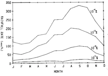
Alternatively, we can look in detail at the evolution in the values of the intensity R , throughout the months of an average year, which is responsible for a specified outage (percentage of month that indicated R is equalled o r exceeded). The particular result of our investigation is shown in Fig. 11 where we clearly see the worst calendar months for a radio link as well as the optimum ones. However, if we are not concerned with extreme values ( P 2 IO-’ percent), then all months look equally favorable. Undoubtedly, similar investigation could be carried out for other CCIR zones provided that real monthly distributions can be obtained.

The study has also included for completeness the relation between the average annual P I 3 ( R ) and each one of the various P i ( R ) i = 1

. . .

12 as given by an equation of the form

-

P i ( R ) = A ( P 1 3 ( R ) ) b

(7)

This is naturally convenient for our CCIR zone L to where Catatonia belongs, but it will be of little use worldwide.

390 IEEE TRANSACTIONS ON COMMUNICATIONS, VOL. COM-35, NO. 4. APRIL 1987 TABLE I

VALUES OF THE PARAMETERS A AND B RELATING WORST MONTH AND MONLTHY DISTRIBUTIONS TO THE ANNUAL DISTRIBUTION (SEE (7) AND

MONTH JANUARY FEBRUARY MARCH A P R I L MAY J U N E J U L Y AUGUST S E P T E M B E R OCTOBER NOVEMBER DECEMBER WORST TEXT) - A b

2.5546

1.3512

48.6673

1.7028

30.2329

1.5951

5.9522

1

.,3011

11.2916

1.3180

1.0146

0.9839

0.6842

0.9464

0.5503

0.8609

1.3441

0.9372

2.5737

1.0186

0.9247

0.9952

3.5619

1.2405

1.3352

0.8477

Nevertheless, Table I summarizes these values of the parame- ters A and

b

of (7). This allows one to go from the average annual P I 3 to any average calendar month.

v.

HOURLY AND MONTHLY-HOURLY DISTRIBUTIONS Provided that the data bank is available, it will be undoubtedly, very useful to discriminate the yearly intensity outages P,,(R) on the hour of the day inclusive (if possible) of

the calendar month. This will permit to resolve which periods of the year contribute most to the small outages; in other words, we wish to find out the periods whose rain rate exceeds about 50 mm/h. This value is to be compared to the 40 mm/h quoted in [3] and which other authors would also class as a limit for convective precipitation rate. This may be of particular importance to secure high density communications irrespective of the social or unsocial hours of the troughs of

P ( R ) for those seasons (months) when heavy showers may occur. A similar type of consideration could come in the field of civil works and drainage when dealing with heavy storms. As explained in Section 11-B, the hourly evolution of P ( R )

was investigated looking at periods in the day of two successive GMT hours, and then counting the duration of exceedance of the given 80 thresholds. This was done either over the 49-year period, or going further and according to the month of the year (over the 49-year period) looking in detail at the plots R - P 1 3 ( R ) over two-hour periods. For the first type of investigation, the 12 R - P ( R ) distributions were looked at

in detail against the annual average. The plots look similar to those of Fig. 10 in the sense that some distributions are above the annual average and others are below. Alternatively, and without selection on month or season, we can look at the evolution of R throughout an average day for each outage

selected. This is shown in Fig. 12. Here we see the impact of convective rain contributing mainly to the small percentages of time. W e see for example that low values of R are completely independent of the hour of occurrence (as was the case in Fig. 11 for the month of the year) whereas for very small

percentages of time, values of

R

in excess of about 150 mm/h are very dependent on the time of day (as again it was in Fig. 11 for the month of the year). We see the particular feature that these very heavy rates are produced in the evening or early hours in the morning. As shown by Fig. 12, some months do not exhibit high values of R even for low outages and therefore the statistics of Fig. 12 are smoothed out by this effect in the sense that maxima and minima (troughs) are contributed

400 t . t 350

1

a 300

5

250 D

-

r- r a 200 ;;I 150 > h 3

$

100 Y 50 n 10-k

AI

equally by months either with or without convective (heavy) precipitation.

The above study leads naturally to resolving the hourly evolution of P I 3 in terms of the month over the 49-year period. In other words, we are lead to study Figs. 12 and 13

simultaneously and thus avoid the statistical smoothing due to those months with mostly low rain rate.

Unfortunately, we have now a four-dimensional problem; that is, for communication purposes, given a certain percent- age of the year, the question is to determine the threshold R responsible for this outage as month and time of the day go by. The massive data bank investigated in this paper has permitted to look at this in some detail, and two types of plots have been looked at. As there are 12 pairs of hours per day in a 12 month (year) period we have a total of 144 possible distributions.

The first type of result is illustrated in Fig. 13(a)-(d) which show in four 3-D plots the evolution discussed above.

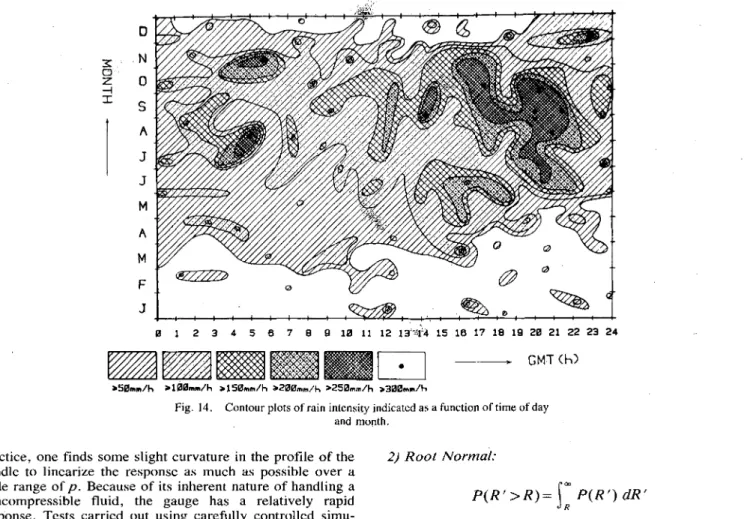
Naturally these results are typical only of the region consid- ered (zone L ) but they show for the indicated percentage of the average year the evolution of the features of Figs. 1 1 and 12. Alternatively, and as shown in Fig. 14, we can plot the shaded contours which enclose precipitation rates exceeded. Here, the code for the grey level (and hence a given R exceeded) will correspond to an annual outage which we can determine, for example, from Fig. 3. In agreement Figs. 11 and 12 we see again that lo-' percent (3.6 min in the 3600 min of a 30-day month in an average year) 3-D plot hardly shows any heavy precipitation rate; the hourly evolution is practically constant for the months of August, September, and October. Similar features are exhibited by the 3 X

lo-*

percent. However, the

lo-'

and 3 X percent 3-D plots confirm that for the geographical zone studied, the light rain rates predominate in January, February, and March, that the important showery months are June, July, August, September, October, and

November, and that for these six months the very heavy rain occurs mostly in the afternoon and then at night-and the early hours of the morning. Thus for example, and given the freedom of the time slot, we should plan any massive microwave communications data transfer for Catalonia in the morning.

VI. DISCUSSION AND CONCLUSIONS

Because of the availability of nearly 50 years of continuous precipitation rate obtained with a rain gauge of 10 s of response time, this paper has investigated in detail several aspects associated with rain-rate data acquisition and related aspects of communication planning statistics.

I

BURCUERO et ai.: ANALYSIS OF MODERATE AND INTENSE RAINFALL RATES

m

c

392

IEEE TRANSACTIONS ON COMMUNICATIONS, VOL. COM-35, NO. 4, APRIL 1987

rainfall intensity over the 49-year period and which covers intensities ranging from a few mm/h well into more than 150 mm/h, unusual in Europe but not in Catalonia, has shown that the modeling by a log-normal distribution is not suitable for precipitation rates above about 60 mm/h. The study of the gamma distribution extended the good fit into the high values of R provided that R

>

25 mm/h confirming earlier findings by other authors. This is a limitation because regions like Europe often have rain rates less intense than this value. T o get a better fit over the whole range, from a few mm/h to well beyond the 250 mm/h, we require a three-parameter distribu- tion such as the Pareto distribution investigated. An important result of this investi ation has been to find that if we use as functional of R the

h,

then the normal distribution of

6

fits the experimental distribution very well within 10 percent up to 170 mm/h, and nearly to 250 mm/h if we extend the tolerance to 20 percent of error (Fig. 4). This distribution is simple to handle and use and we would recommend it for serious consideration as an alternative model covering low and high R ’ s . In order to extend or compare the specific numerical results of the cumulative probabilities for a given R to other locations, one must bring in the average fraction of the time (year) that it rains. Our fraction was 1.21 percent.

Each one of the 80 chart threshold levels in which our 0-474 mm/h range was investigated, had an annual cumulative probability value (outage) P ( R ) associated. There are 49 values (covering the period 1927- 198 1). This has permitted to address in detail the statistics of the spread of these P ( R ) values. By averaging P ( R ) in independent groups of an increasing number of. years it has been found that no less than seven years, and preferably ten, are required before the

various average distributions cluster towards a common final one (the one over 49 years) which naturally shall reflect the geographical location and zone. Furthermore, by investigating for each R the distribution of the 49 values of the ensemble [ P ( R ) ] it was found, in agreement with Segal of Canada, that these values had a cube-root normal distributiqn. This permit- ted establishing a parametric study of margins of statistical confidence (Fig. 8), and to determine return times to a P ( R ) distribution greater than o r smaller than some specified boundaries (Fig. 9). For example, the comparison between Figs. 8 and 9 show that the -t- l a and - l a spread of the distribution of P ( R ) ’ s for R = 75 mm/h corresponds (approximately) to a return time

N

and

N’

of 6.3 years. If we extend the range to

+

2 a and - 2 a then the return times

become 44 years.

These results are vital to plan a campaign of rain-rate data acquisition with statistical criteria supporting the decision. Perhaps it is relevant here to bring in the consideration of balancing complexity of the gauge, its maintenance and data retrieval; there is no doubt that if the Jardi gauge had not had the characteristic of simplicity of maintenance and had it not been located in an observatory securing uninterrupted un- skilled maintenance, the data bank would have had the usual problems of interrupted recording. The authors believe that the balance tilts in favor of continuous and reliable manpower irrespective of the level of skill and therefore the gauge must match the technical skill of the caretakers for long-term investigations over many years.

The study of the subject of the synthetic worst month recommended by the CCIR has been looked at in detail. Experience from previous work on the same subject shows that there is no difficulty in mapping the average annual distribution to that of the worst month one via a relation of the type A [ P I 3 ( R ) l b . However the worst month looks at extreme values of P ( R ) irrespective of the time of occurrence and this is why in this paper a closer look was taken resolving the P ( R ) in terms of its calendar month contributions. As a result it was found that several groups had an average P ( R ) which was above the annual P ( R ) and some others were below but at all

times they were less than the P ( R ) of the worst month by at

least a factor of 2 and increasing to 5 for R

>

100 mm/h. The recommendation therefore is that if the data bank is available, the calendar month distributions over the years should be closely investigated to avoid the risk of over-estimating outages and thus over-designing microwave radio-communi- cation systems.

The investigation of the P ( R ) for the various calendar months over the years reveals the importance of those months with a great probability of convective rainstorms (August, September, and October in our particular zone). This has led to investigating in detail the hourly evolution of R , given a specific outage, as time of day and month of the year go by. This study of the fine structure of P ( R ) was carried out using both 3-D representation and contour plots (Figs. 13 and 14). The results, although only applicable to Catalonia and more generally to the northwest of the Mediterranean sea (zone L CCIR), indicate the power of this type of statistical .analysis from which a radio-communications planning can now be undertaken with confidence.

APPENDIX I The Jardi Rain-Rate Gauge-Static Response and Calibration

In the early 1920’s, at the request of the Catalonia Local Authority and Meteorological Service, a rain rate gauge was designed by Professor R. Jardi for flood forecasting and civil works planning. The original description and basic operation can be found in [ 101-[12]. The gauge, which is no longer manufactured, gives chart recordings of R in mm/min and was designed to monitor the intense precipitation rates which occur in the northeast of Spain. One should note that in civil works and Telecommunications what matters most is the rate of rainfall, and the Jardi gauge was the first rapid response rain- rate gauge designed. Fig. 15 shows a diagram of the instrument. A very brief description of the inst.rument can be found in English in [13]-[16]. This instrument is still in operation at the Fabra Observatory, and operates in the following way. The rainfall collected by a large funnel of section So (0.18 m?) flows to a chamber where a float rises to a

given level (response), due to the input flow (signal). As the float rises, the opening of variable area a R 2 - ar2 increases

due to the conical shape of the stindle which blocks the orifice of radius R . This movement continues until input‘and output flows are equal and the movement of the float is recorded on a daily chart attached to a revolving drum. If

4

is the input flow of water in, say, cm3/min then

4

is given by the flow velocity u = &g(h

+

a ) times the clearance a R Z - a r 2 . We also note that

4

is given by the product p S o where p is here the rain rate in cm/min. One can easily show that if the stindle blocking the orifice has a conical shape so that the radius r for a given position h is given by R(1 - h,’l), then we get the -basic equations for the gauge relating the rain rate p to the displacement h (recorded)

p = u o - ~ [ 2 X - X 2 ]

SI

O<X<1

(A-1)

S

O

with X = h / l , S , = a R 2 , A = a / l , u, =

m,

and with g the gravity acceleration constant. If we keep

I

+

h and I

+

a SO

that the orifice is closed by the part of the stindle closest to the base .of the cone, then (A-1) can be approximated by the relation

p=2u0

-a

SI

x

SO

(A-2)

BURGUERO e1 ai.: ANALYSIS OF MODERATE AND INTENSE RAINFALL RATES

393

f(

cl

Z 4 I D N 0 S A

J

J

M A M F

J

.SBrm/h >lBBmm/h >15Eimm/h X?BBmm/h > 2 5 0 m m / h > 3 B B m m / h

Fig. 14. Contour plots of rain intensity indicated as a function of time of day and month.

practice, one finds some slight curvature in the profile of the stindle to linearize the response as much as possible over a wide range of p . Because of its inherent nature of handling a noncompressible fluid, the gauge has a relatively rapid response. Tests carried out using carefully controlled simu- lated values ofp have shown that the Fabra Observatory gauge has just under 10 s response time to go from 10-90 percent of the final value after applying a step input A p . T o reach the final steady value we measured about 20 s. One notices that the gauge operates as a mechanical control system in which the restoring force to a constant input flow

4

is the difference between the buoyancy of the float and its weight (inclusive of any friction in driving the pen-recording mechanism).

APPENDIX I1

Modeling of the Average Annual Distribution

The research in the mathematical modeling was carried out first by plotting the average annual cumulative distribution in its conventional form Prob (R’

<

R ) = 1 - P ( R ) using probability paper. In abscissas, one plots the reduced variable (number of sigmas) and in ordinates a functional of R (to be determined). In this way, InR was found to be normally distributed for the range 12-60 mm/h. However, a better straight-line fit within the range 18-170.5 mm/h was obtained using as functional of

R ,

_G.

The two distributions 1) and 2) in conventional outage form can be written as

I ) Log Normal:

P ( R ’ > R ) =

P ( R ’ )

d R ’

R > O

U I ~ R

J

2) Root Normal:

P ( R ’ > R ) =

im

P ( R ’ )

dR’

(A2-2)

-

with now R ” 2 = - 23.225 and uR1/2 = 8.325. Good fit within the 10 percent exists well up to 170 mmyh.

3) Gamma Distribution: This distribution is favored for large precipitation rates. The, technique to determine the distribution has been discussed elsewhere [ 181 by Boithias. By calling X a convenient reduced variable R / R , he then finds the following approximation

,-X c = = Y

X + 0.68

+

0.28

loglo

X

(A2-3)

An iterative technique gave R , = 54 mm/h and v = 5.7 X

and the approximation to the experimental curve was within 10 percent provided that R

>

24 mm/h.

4) Generalized Pareto Distribution: The distribution proposed by De Reffye [25] approximates a log-normal distribution at low rates and gamma distribution at high rates and includes the power law of Segal [22]. The distribution can be written as

with P ( R ) the p r o b a E t y density or frequency function distribution. By using InR = -6.538 and u l n R = 2.880 (A2-

1 ) was found to fit P , , ( R ) .“. , in the range 12-60 mm/h with relative differences less than 10 percent.

I

394

IEEE TRANSACTIONS ON COMMUNICATIONS. VOL. COM-35, NO. 4, APRIL 1987 300 78 \

I

I

t

Fig. 15. Principle of operation of the Jardi rain rate gauge (to scale).

and fits our experimental

p13

within 10 percent, well beyond

260 m p / h provided that R

>

12

mm/h. The constants found were CY .= 2.098 X mm/h, v = 0.818, and p = 1.765 X

lo:* ( m m h - ! (a = 8.418 X b = 0.818).

* .

APPENDIX 111

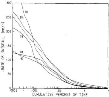
As explained in the text, for reasons of homogeneity, the years 1930 and 1978-1981 were excluded from the overall analysis in’ligh; of the comparison and discrepancies shown in Fig.

2 .

Nevertheless, Fig. 16 shows the five cumulative distributions of those five years, and they have been included in this paper for ‘ t h e sake of completeness an4 possible reference.

ACKNOWLEDGMENT

This paper is part of a cooperative venture between Portsmouth Polytechnic and the University of Barcelona and several organizations have contributed to its. success. The Barcelona group is grateful to the CIRIT of the Generalitat

I

\\\\

79‘

.Q

CUMULATIVE PERCENT OF .Ol

TIME

.I 1

Fig. 16. Cumulative distributions of the years not considered in the study (-. -) 49 years mean distribution.

Government of Catalonia and to the Spanish Advisory Committee for Scientific and Technical Research. The Ports- mouth group is grateful to the British Council and to the Polytechnic. Special thanks are due to colleagues and students for the painful digitizing process, in particular, S . Alonso, M.

C . Llasat, and A. Redano. Special thanks are also due to J . R . Norbury of RAL for useful information and to the Director of the Fabra Observatory, J. M. Codina, for the facilities and access’to the Jardi recordings.

REFERENCES

R. L. Olsen, D. V. Rogers, and D. B. Hodge, “The a R b relation in the calculation of rain attenuation,” IEEE Trans. Ant. Propag., vol. AP- 26, no. 2, pp. 318-329, 1978.

R: K . Crane, “Prediction of attenuation by rain,” ZEEE Trans. Commun., vol. COM-28, pp. 1717-1733, 1980.

P. L. Rice and N. R. Holmberg, “Cumulative time statistics of surface point rainfall rates,” IEEE Trans. Commun., vol. COM-21, pp. H . T. Dougherty and E. J. Dutton, “Estimating year-to-year variability of rainfall for microwave applications,” IEEE Trans. Commun., vol. COM-26, no. 8, pp. 1321-1324. 1978.

E . J. Dutton and H. T. Dougherty, “Year-to-year variability of rainfall for microwave applications in the U . S . , ” IEEE Trans. Commun., vol. COM-27, no. 5 , pp. 829-832.

CCIR, “Attenuation by hydrometeors in particular precipitation and other atmospheric particles.” Rep. 721-1, Question 215, 1978-1982. B . N. Hqrden, J . R. Norbury, and W. J. K . White, “Measurements of rainfall for studies of millimetric radio attenuation,” Microwaves Opt. Acoust., vol. 1, no. 6, pp. 197-202. 1977.

J. R. Norbury, “A.rapid response rain gauge for microwave attenua- tion studies,” J . de Rech. A t . , vol. 8, pp. 245-251, 1972.

S. H . Lin. “Dependence of rain-rate distribution on rain gauge integration time,” Bell Syst. Tech. J., pp. 135-141, Jan. 1976. R. Jardi, “Un Pluviograf d’htensitats,” Notes d’Estudi, Servei Meteorologic de Catalunya, vol. I, no. 2, pp. 3-10, Barcelona 1921. E. Fontsert, “Intensitats-pluviograph nach Jardi,” Meteor Zeits., vol. 39, p. 89, 1922.

R. Jardi, “Estudis de la Intensitat de la Pluja a Barcelona,” Memories de 1’Institut d’Estudis Catalans, vol. I, Fasc. 11, Barcelona, pp. 51-76, 1927.

Handbook of Meteorological Instruments, Part I, Meteorological Office, London, England, 1956.

W. E. K . Middleton and A. F. Spilhaus. Meteorological Znstru- ments. Toronto, Canada: Univ. Toronto Press, 1953.

A. Perlat and M. Petit, Measures en Meteorologie. Paris, France: Gauthier-Villars, 1961.

G . G. Rossman and J. M. Wardle, “The Hudson design-Jardi type 1131-1136. 1973.

BURGUERO et ai.: ANALYSIS OF MODERATE AND INTENSE RAINFALL RATES

395

recording rain intensity gauge and rainfall totaliser.” Bull. Amer.

Met. Soc., vol. 30, no. 3, pp. 97-103, 1949.

[I71 CCIR: Recommendation AJi5, Doc. 5/1033-E, September 1981. 15th Plenary Assembly, Geneva, Switzerland, 1982.

[I81 L. Boithias, “On the statistical distribution of rain rate,” Ann. des Telecotntn., vol. 35, pp. 365-366, 1980.

[I91 S. H. Lin, “Rain rate distributions and extreme value statistics,” Bell Syst. Tech. J., vol. 55, no. 8, pp. 1111-1124, 1976.

[20] F. Fedi, “Attenuation due to rain on a terrestrial path,” A h Frequenza, vol. XLVIII, no. 4, pp. 167-184. 1979.

[21] -, “Prediction of attenuation due to rainfall on terrestrial links,” Radio Sci., vol. 16, no. 5, pp. 731-743, 1981.

1221 B. Segal, “An analytical examination of mathematical models for the rainfall rate distribution function,” Ann. des Telecom., vol. 35, no. [23] K. Morita, “Study of rain rate distribution,” Rev. Electron. Com- [24] CCIR. “Radiometeorological data,” Rep. 563-2, Question 215, 1974- 1251 J. De Reffye, “Modelisation mathematique des intensites de pluie en un

point du sol,” Rev. Statistique Appliquee, vol. XXX, no. 3, pp. 39- 63, 1982.

[26] F . Moupfouma and J . De Reffye, “Empirical model for rainfall rate distribution,” Electron. Lett., vol. 18, no. 11, pp. 460-461, 1982. [27] -, “Two parameter empirical model for rainfall rate distribution,”

Electron. Lett., vol. 19, no. 19, pp. 800-801, 1983.

[28] T . J . Moulsley and E. Vilar, “Experimental and theoretical statistics of microwave amplitude scintillations on satellite down-links,’’ IEEE Trans. Ant. Propag., vol. AP-30, no. 6, pp. 1099-1106, 1982. [29] B. Segal, “The estimation of worst month precipitation probabilities in

433, 1980.

microwave system design,” Ann. des Telicomm., vol. 35, pp. 429- [30] M. Puigcerver, S. Alonso, J. Lorente, and E. Vilar, “Long-term

precipitation rate statistics for north-east of spain,” Electron. Lett., vol. 19, no. 4, pp. 129-130, 1983.

11-12, pp. 434-438, 1980.

mun. Labs., vol. 26, pp. 268-277. 1978. 1978-1982.

*

August BurgueFio was born in Barcelona, Spain, in 1957. He received his meteorological education at the University of Barcelona, from which he re- ceived the degree in physics in 1981.

He has completed his doctoral dissertation on rainfall rate statistics at that University, and in connection with that research, he has also worked in the Electrical and Electronic Engineering Depart- ment of Portsmouth Polytechnic (U.K.).

Dr. Austin is a Chal Electrical Engineers (U.

John Austin was born in Wiltshire, England and graduated with the first class honours degree in electrical and electronic engineering from Ports- mouth Polytechnic in 1968.and the Ph.D. degree in electrical engineering in 1973.

He is currently a Senior..Lecturer at Portsmouth Polytechnic and a memb&&of the Microwave Telecommunications and Signal Processing Re- search Group. His main interests are computer systems and digital signal processing applied in a variety of disciplines.

tered Engineer and a member of the Institution of K.).