3D Object Recognition from a Single Image via Patch Detection by a Deep CNN

(1)

ALMA MATER STUDIORUM

UNIVERSITY OF BOLOGNA

SCHOOL OF ENGINEERING AND ARCHITECTURE

Second Cycle Degree in Automation Engineering

THESIS

in

Computer Vision and Image Processing

3D Object Recognition from a Single Image via Patch Detection

by a Deep CNN

CANDIDATE SUPERVISOR:

Francesco Taurone Chiar.mo Prof. Luigi Di Stefano ADVISORS Dott. Daniele De Gregorio Dott. Alessio Tonioni

Academic year 2018/19 Graduation session I

(2)

(3)

To my family, for supporting me.

(4)

(5)

Introduction

Pose Recognition is the task of understanding the position and orientation of an object in space with respect to a world reference frame by means of a series of pictures taken from a camera. Therefore, the desired result is an estimation of the rototranslation from the camera reference frame to the object reference frame, namely a description of the object position and orientation with respect to the camera taking the pictures.

Pose recognition has proved to be a key element for many tasks involving computer vision, since it is necessary whenever the task to be accomplished requires interactions with objects.

As a matter of fact, there are many possible examples of use of pose estimation in various contexts, such as:

• Industrial manipulators, that are required to grasp objects placed in random po-sitions and orientations, which usually makes use of a camera on the end-effector. Since the grasping points depend on the object itself, it is important to estimate the pose of the object in order for the robot to handle it correctly.

• Augmented reality applications, for various contexts such as industry, gaming, etc. It is key to recognize the surrounding environment, as well as the objects placed therein.

• Quality control, to check the final position and orientations of goods at the end of a production line.

• Physiology, to track the posture of human bodies for analysis, for rehabilitation, etc.

This thesis targets the pose recognition of an object in space by using the recognition of a series of patches in an image of the object, for which a Deep Network is trained. This, together with the association between labels of the keypoints and their 3D coordinates with respect to the object, allows the estimation of the pose in space. In order to cre-ate the training dataset for the deep learning network, this thesis proposes an innovative semi-automatic learning technique, adapted from previous theses for this particular task.

(8)

(9)

Abstract

This thesis describes the development of a new technique for recognizing the 3D pose of an object via a single image. The whole project is based on a CNN for recognizing patches on the object, that we use for estimating the pose given an a priori model. The positions of the patches, together with the knowledge of their coordinates in the model, make the estimation of the pose possible through a solution of a PnP problem. The CNN chosen for this project is Yolo [10].

In order to build the training dataset for the network, a new approach is used. Instead of labeling each individual training image as for the standard supervised learning, the initial coordinates of the patches are propagated on all the other images making use of the pose of the camera for all the pictures. This is possible thanks to the use of AR-Core package by Google and a supported phone like the Pixel, upon which this thesis and others have developed an app for keeping track of the pose of the phone while moving.

At this stage, this project is intended to recognize single objects in the space. It could be generalized to recognize multiple objects as well.

In order to summarize the results achieved with this thesis, following is a brief de-scription of the whole proposed pipeline to recognize the 3D pose of an object.

• Train the Net (Yolo):

1. Choose the keypoints and extract their coordinates:

In order to identify the keypoints on all the captured image, an initial set of coordinates to be propagated is needed. For this thesis, a CAD of the object has been used in order to measure the position of the chosen points of interest to be tracked, but they could also be measured manually (in which case, for the following steps involving CAD, a carefully placed cube can be used). The choice of the keypoints is made by the user. The effect of the number of keypoints to choose for each object , as well as the suggested characteristics, are discussed in a specific section 2.2.

2. CAD of the object to be recognized :

It needs to be imported on the phone where the app for generating the dataset is installed.

(10)

3D pose recognition via single image based on deep networks 3. Position the CAD in the App on the scene:

The app needs to be installed on the phone via APK. The phone needs to be a ARcore supported device, in order to have a precise tracking while capturing. The CAD is then asked by the app once launched, it needs to be positioned in correspondence of the real object in the scene, so that they overlap.

4. Record and save the resulting files:

Once the recording button is pressed, a series of images is saved according to the selected frame rate. For each image, the pose of the camera is saved in a file. For each record, the initial position and orientation of the object are saved on a file. These files are going to be used to generate the training dataset for Yolo.

5. Generate the dataset:

Beside the images, in order to train Yolo there’s the need of a series of labels for each image. This labels are generated automatically, since both the pose of the camera with respect to the world and the pose of the object with respect to the world are known. This assumes that the object is not moving while the training set is generated, and that the camera is tracked quite precisely. 6. Train Yolo:

Once the positions and labels of each patch for each image have been generated, the command to train Yolo can be launched.

• Recognize the pose of the object with the trained net for each image: 1. Detect the patches:

Running Yolo on each images, a set of patches is identified. 2. Get the position and orientation of the object:

Once the keypoints are identified, a PNP using ransac is launched. Since for each label there is a correspondence between the detected keypoint and the coordinates in the nominal model, namely the CAD, it is possible to retrieve the pose of the object. The final result is therefore a translation vector and a rotation matrix, that represent respectively the position and orientation of the object with respect to the world.

This project has been developed using Python, for processing data and network train-ing, Java for the android App.

The software used are PyCharm as IDE, Android Studio for the android app, Blender for the 3D models and model reprojection on images, LabelImg for manual labeling in the prototype, Putty for remote training of the Deep Network, Excel for data analysis. 10 Chapter 0 Francesco Taurone

(11)

Chapter 1 Pose Recognition - State of the art

Pose Recognition has quickly become a key element for all sorts of newer technologies involving vision, since it is one of the basic tasks to be performed for most of augmented reality applications (AR).

As analyzed in [1], this is a quite old problem, that has been solved in various ways during the last 25 years. The first attempts made use of classic computer vision techniques relying on markers, to be tracked during the motion of the camera. However, this approach lacks flexibility, since these markers have to be attached to the object itself, which might not always be possible.

For this and other reasons, markerless approaches started to become more popular in the scientific literature. Since this thesis aims the estimation of poses of 3D object without making use of markers, in the following a brief overlook at some of the most well known approaches to markerless pose estimation.

Approaches to 3D pose recognition

Some of the most common approaches for dealing with pose recognition are:

• Known 3D model: the idea is to fit in the best way a known 3D model of the object to be analyzed in the scene. This makes use of techniques like P3P, using 3 points, or PnP, with n points, with or without RANSAC (Random Sample Consensus) to deal with outliers. Alternatives to RANSAC are M-estimators, which are generalized versions of Maximum likelihood and Least squares. One of the most common setup is indeed Pnp without any initialization (EPnp) alongside RANSAC, that is the approach used in the thesis.

• Match low level features: since each object has some key elements that our brain perceives as unique and characteristic, the some idea is translates in computer vision as keypoint matching. These features have to be extracted from the model first, then paired with the keypoints in the image basedon a descriptor. These pairs make the pose estimation possible.

(12)

3D pose recognition via single image based on deep networks

There are indeed many proposed methods for the automatic extraction of features and the relative descriptors. Beside SIFT [2], which was a major breakthrough for 2D points matching, SURF and FAST are some of the most successful and recent feature extraction algorithms available to the scientific community, especially for AR applications. For building the descriptors instead, many methods have been proposed and compared for computational efficiency and result effectiveness once matching is performed.

Recently, latent modeling approaches have been proposed to learn optimal sets of keypoints without direct supervision [3]. Some have tried to make the detection of effective keypoints a less labor intensive process [4]. This thesis uses user chosen keypoints, and leaves the automatic selection of those as further development in 4.1. Quick overview about camera pose estimation

For the sake of this thesis, in order to propose a semi-supervised technique for deep network dataset creation, we make use of tracking techniques for the estimation of the pose of a moving camera in the environment.

The tool employed to estimate the camera pose is ARCore by Google, which makes use of a concept developed in the late 2000s and still quite an active research topic named SLAM (Simultaneous Localization and Mapping) that allowed the localization of the camera while it is moving in the environment.

SLAM does not make use of a priori model, which is not always available, but rather tracks the motion of the camera with respect to the environment, so to retrieve the pose of the object as well. The main issue with this approach is the lack of an absolute localization and its cost inefficiency in large environments. Some hybrid approaches partially cope with these problems, making use of an online PnP.

1.1 Examples of successful algorithms for 3D Pose

Estimation

Many elegant and interesting solutions to 3D Pose estimations have been proposed in the recent past.

Some of the most representative algorithms are:

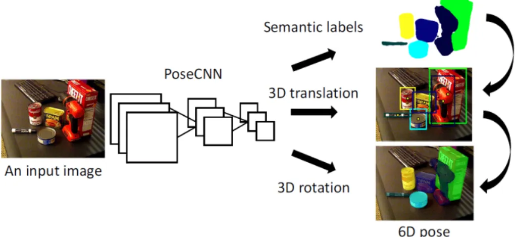
• PoseCNN [5]: it is one of the first approaches to 3D pose estimation, and works by estimating the 3D translation of an object by localizing its center in the image and predicting its distance from the camera. The 3D rotation of the object is estimated by regressing to a quaternion representation. The structure is represented in Figure 1.1

(13)

Figure 1.1: PoseCNN structure

• SSD-6D [6]: This is an extension to the to the SSD paradigm to both position and orientation of the object, therefore covering all the 6 degrees of freedom of a rigid body in 3D space. Here the stages are: (1) a training stage that makes use of syn-thetic 3D model information only, (2) a decomposition of the model pose space that allows for easy training and handling of symmetries and (3) an extension of SSD that produces 2D detections and infers proper 6D poses. This is therefore a method alike the one developed in this thesis, namely based on single RGB images. Additionally, SSD-6D can be easily extended to RGB-D images, including distance information. This is indeed approaching the pose estimation problem as a classification task. See figure 1.2 for the structure of the network.

Figure 1.2: Schematic overview of the SSD style network prediction. The network is fed with a 299x299 RGB image and produce six feature maps at different scales. Each map is then convolved with trained prediction kernels to determine object class, 2D bounding box as well as scores for possible viewpoints and in-plane rotations that are parsed to build 6D pose hypotheses.

• BB8 [7]: This method uses RGB info as well, and solves the pose estimation task Francesco Taurone Chapter 1 13

(14)

by inferring the 3D points of the bounding box for the chosen object. Namely, it applies a Convolutional Neural Network (CNN) trained to predict their 3D poses in the form of 2D projections of the corners of their 3D bounding boxes. Like Yolo, the net for image recognition used throughout this thesis, BB8 splits each image into regions, extracting binary masks for each possible object. The largest component is kept, and its centroid is used as the 2D object center. Then, in order to estimate its 3D pose, the chosen segment centered in the centroid is fed to a Deep Network, thus achieving both position and orientation. Some refinement is required to get a more precise estimation. Example of results in figure 1.3.

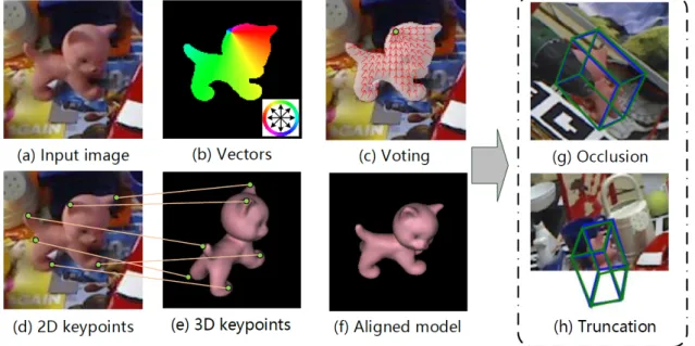
Figure 1.3: BB8: some qualitative results with different shapes and occlusions. • PVNet [8]: Similarly to BB8, PVnet infers points of the object to retrieve its 3D

pose. The method PVNet employs is a Pixel-Wise Voting Network to regress pixel wise unit vectors pointing to the keypoints, using then these votes to retrieve the keypoints locations through RANSAC. Ones the keypoints are selected by voting, a PnP is applied to get an estimate of the 3D pose. This method proves to be partic-ularly effective against occlusions and truncation, since the visible pixels contribute to the voting process nevertheless. See Figure 1.4.

Chapter 2 will be devoted to the development of the final pipeline that this thesis presents, as well as the solutions to the challenges faced in the process.

(15)

Figure 1.4: PVNet: the different steps of the process.

(16)

(17)

Chapter 2 Development of the algorithm

This thesis aims to assess whether a patch oriented 3D pose algorithm can compete with other approaches, like the ones seen in 1.

The main motivations for researching on this approach are: 1. Versatility:

Even if for this thesis Yolo has been chosen as the Deep Network to recognize patches, it is nonetheless non ideal for these purposes. Another more specialized network could be chosen as a substitute, given some performance requirements. 2. Robustness to occlusions and truncation:

Since few object points, and therefore few patches, are required to reconstruct a pose via PnP, even when the object is occluded the estimation process is expected to perform satisfactorily.

3. Quick training via a custom AR based app:

In order to obtain a dataset to train the network of choice, only few minutes are required. The development and use of the app in 2.3.

4. Many further direction of development:

As listed in 4.1, there are many possible ways to improve the performances of the current algorithm (for example, an automatic way for determining the best keypoints to choose).

In the following, a description of the elements needed for this pipeline.

2.1 Choice of the network

Since the main objective is to develop a patch oriented system for recognizing the pose of an object in 3D, there is the need to choose a reliable network able to detect multiple patches of various dimensions on single RGB images in real time.

(18)

Yolo has proved itself as state of the art in the last months for what concerns detection on images. Moreover, the community behind the development and maintenance of this software is particularly active on platforms like GitHub. Yolo returns as output also the confidence level of its predictions, which is very useful to label only the most probable detection as object keypoints.

The chosen implementations for this thesis can be found here [9].

2.1.1 What is Yolo

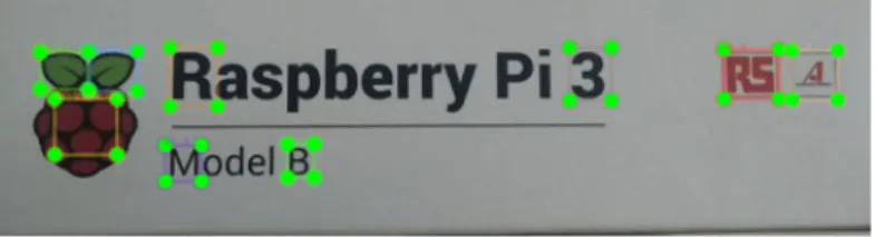
As described in [10], ”You Only Look Once” (YOLO) is a state-of-the-art, real-time object detection system. A single neural network is fed with the full image. This network divides the image into regions and predicts bounding boxes and probabilities for each region. These bounding boxes are weighted by the predicted probabilities.

It looks at the whole image at test time so its predictions are informed by global context in the image. It also makes predictions with a single network evaluation unlike systems which require thousands for a single image. This makes it a very fast network.

An example of output is in figure 2.1, where bounding boxes for the objects present in the scene are drawn.

Figure 2.1: Example of Yolo output

Moreover, Yolo returns the confidence level of each prediction. Quite naturally, the higher the confidence level, the more likely it is a trustworthy prediction. This is a key element for choosing Yolo against other detectors, since this index proves to be useful when multiple instances of the same patch are detected, but only the most trustworthy can be label as the corresponding object keypoint.

(19)

2.2 Prototyping with a simple object - the raspberry

box

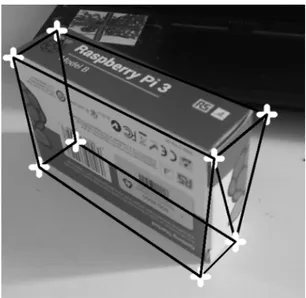
In order to test the capabilities of this approach and to understand its critical points, we first test the net on a simple object, a box. We choose the Raspberry box in Figure 2.2 with noticeable elements on it, that would serve as patches samples.

Figure 2.2: The Rasperry Box used as prototype

The objective of the test is to map the different 2D sides of the box on the 3D image based on the detected patches. More specifically, once the pairs of patches are obtained, one from the side image and one from the box in space image, the centroid of those patches are used as keypoints to perform an homography based on the matches, mapping 3D boxes’s keypoints with side’s keypoints.

The homography represents an intermediate step with respect to the complete PnP, since it exploits the fact that the thing to be projected in space is a plane surface, having therefore less degrees of freedom.

The steps for the tests were:

1. Take pictures of the sides (image of a 2D object) and of the box in space (image of a 3D object). The needed set of images are:

(a) Images of all the 6 sides, to be labelled manually;

(b) Images of the box in space to be used for training Yolo, and therefore to be labelled manually;

(c) Images of the box in space to test the trained Yolo and the idea of patch based pose recognition.

2. Label the first and second dataset manually, like in figure 2.3 and 2.4. The tool used for labeling manually each image can be found here [11] The criteria to choose patches were:

(20)

Figure 2.3: The Rasperry Box with the patches. Manually labeled.

Figure 2.4: The Rasperry Box Side with the patches. Manually labeled.

• Small compared to the object: since we consider the centroid of a rectangular patch, a big sized patch would result in higher noises after detection;

• Roundish elements as patches: in this way, even when rotated or skewed, the patch would look similar and therefore recognizable by Yolo;

• Spread in the object: it was immediately noticeable from the results that a quite homogeneous distribution of the patches on the object was needed to achieve a good homography. This criteria proved to be even more important for the complete PnP with more complex objects, as reported in 4.

3. Train Yolo on the training set of images to recognize the patches of each side of the box.

An example of Yolo output once trained in Figure 2.5.

4. Perform the homography on the test dataset for all the 6 sides of the box.

The results of these test are comforting. After few adjustments, the idea of using patches detected via Yolo for homographies provides good estimations, since in the ma-jority of cases the homographies resulted in images like figure 2.6 and 2.7.

An example of patches correspondences in Figure 2.8.

However, initially the patches were chosen without taking care of all the criteria for selecting successful sets, resulting in unsatisfactory results like in Figure 2.9.

This proves once again that the choice of the keypoints is critical for the performances of this algorithm.

(21)

Figure 2.5: Example of Yolo output for an image of the side.

Figure 2.6: An example of successful series of homographies.

Figure 2.7: Another example of successful series of homographies.

(22)

Figure 2.8: Homography result for one of the sides of the box, highlighting the corre-sponding patches.

Figure 2.9: An example of failed homographies.

(23)

3D pose recognition via single image based on deep networks The next step was to use a custom app to quickly create datasets in order to train Yolo for more complex objects.

2.3 The App to create datasets

The app is meant to quickly create a dataset of images in order to train Yolo with an automatic labeling technique. This app has been adjusted based on a previous version from [12].

The core toolkit employed to make this possible is ARCore from Google, as well as a compatible smartphone (in this case, a Pixel phone).

2.3.1 ARCore and its use

As presented on Google’s website [13], ARCore is a platform for building augmented reality applications.

ARCore uses three key capabilities to integrate virtual content with the real world as seen through the camera:

• Motion tracking, to understand and track the position of the phone relative to the world;

• Detect the size and location of surfaces in the environment; • Light estimation.

ARCore’s motion tracking uses the phone’s camera to identify interesting points and tracks how those points move over time. With a combination of the movement of these points and readings from the phone’s inertial sensors, ARCore determines both the posi-tion and orientaposi-tion of the phone as it moves through space.

Basically, ARCore is tracking the position of the mobile device as it moves, allowing the user to know the position of the phone with respect to the world frame, assigned a priori by the tool.

Since the final objective of this app is to estimate the pose of the phone with respect to the object, or vice versa, the world frame assigned by ARCore is not really meaningful, since it will not be accounted on the final frame transformation.

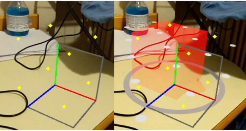
An example of how ARCore places objects in the environment in Figure 2.10.

2.3.2 The use of the app

A custom app is created so to record the pose of the camera and of the object in the environment during the shooting of the dataset. The main idea is to place a CAD model of the object in the environment, so that it overlaps with the real object. This allows us Francesco Taurone Chapter 2 23

(24)

Figure 2.10: An example of a 3D object placed in the environment using ARCore. to keep track of the position and orientation of the model, and then to propagate it for each image shot in the process by means of the camera poses.

The propagated coordinates of the keypoints, once projected on each image, will cor-respond to the keypoints of the real object, since CAD model on object overlap. These data processing steps are analyzed more in detail in 2.4.

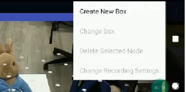
The procedure for recording a dataset is represented in figure 2.11, and described in the following:

(a) Let the app recognize the surface on top of which the object is lying. This step is achieved once a series of grayish dots appear on the desired surface. This step is important in order to keep track of the object even when the camera is moving, namely while performing the proprietary SLAM like procedure. See 2.11a.

(b) Open the menu and select ”Create New Box” to import AR object. See 2.11b. (c) Select Generic, which means that the imported object will be the one previously

added as resource in the app, and then Create. In order to include a personalized model, for now it is necessary to use AndroidStudio and import the asset manually. As further development, the possibility to include an object from Google Drive. See 2.11c.

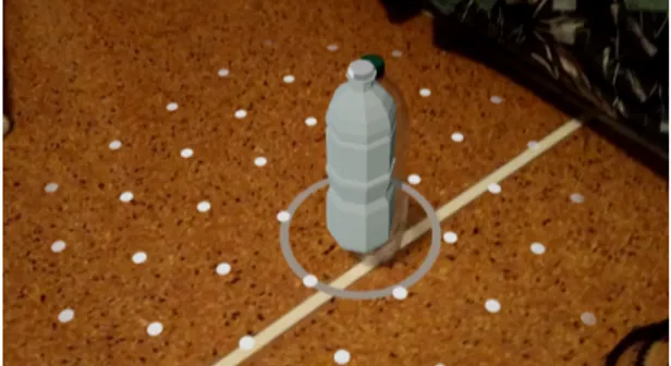
(d) Place the 3D CAD object, previously uploaded on the app, on the highlighted surface. Make the CAD model just added overlap with the real object to shoot by adjusting its position on the plane, its orientation and its scale manually. This app allows pinches and gesture for scaling and moving. See 2.11d. Another example of this step in figure 2.12, representing the image of a bottle as subject for the training before and after placing the model.

To be noted on Figure 2.12b is that the center of the reference frame assigned to the object is highlighted by a grey circle, whose size depends on the chosen scale. 24 Chapter 2 Francesco Taurone

(25)

(a) Main page, the whitish dots are the detected planes to place the AR objects.

(b) Main menu to import the object in the scene.

(c) Select generic and create. (d) Place the model to overlap as precisely as possible with the real object. Adjust scale, ori-entation and position.

(e) Hit the record button. (f) When hit again, a pop up confirms that the

dataset has been created and saved.

Figure 2.11: The main steps to use the app to create a dataset semi-automatically.

(26)

(a) Plain image of a bottle before AR placement. (b) The same bottle as Figure 2.12a, with an overlapping model.

Figure 2.12: Another example of use of the App for dataset creation.

(e) Set the desired frame rate, depending on the desired number of images in the dataset, and hit the recording button, which is red while recording.

By default the frame rate is set to 30 frames per second. Therefore, in order to get a reasonable number of images, like 1000, under this setting we need to record for half a minute.

(f) Hit again the record button to stop the dataset creation. If successful, a pop-up confirmes that the dataset has been saves on the file tree in the phone.

The output files of the app for each dataset will therefore be:

• CameraPose.txt: this file has as many rows as the number of images in the dataset. Each row is in the format

x, y, z, qx, qy, qz, qw

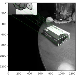
which corresponds to the triplet for translation and the quaternion for rotation. Through these info, it is fairly easy to compute the matrix in projective space representing the rototraslation from the camera frame to the world frame. A visual representation of the camera pose during a dataset recording in 2.13

• Intrinsics.txt: it returns the instrinsics of the camera used to obtain the camera matrix. These parameters are the focal lenghts (fx, fy) in pixels and principal point

(cx, cy), that usually corresponds to the image center.

The camera matrix is important to project 3D point to the 2D image, according to the pinhole camera model.

• Nodes.txt. This contains various information about the models in the environment during the shooting. There are as many rows as the number of models, but for this thesis it is assumed that only one object is present in a given session. In particular, it cointains:

(27)

3D pose recognition via single image based on deep networks x, y, z, qx, qy, qz, qw, id, scalex, scaley, scalez, boxtype

Namely, translation info [x, y, z], orientation info [qx, qy, qz, qw], the id of the model

[id], the scales [scalex, scaley, scalez] that for this application are all equal, and the kind of model considered [boxtype].

Figure 2.13: Visual representation of the content in CameraPose.txt, namely the pose of the camera with respect to the world for each image.

Once the dataset is shot, it is sufficient to downlaod the automatically generated folder from the phone, so to be able to process the data as described in 2.4.

2.3.3 Issues and solutions

• Reference frame direction: unlike standard computer vision applications, ARCore nominally assigns the reference axis to the model as for game development tasks. Namely, the y axis is perpendicular to the surface, whereas the z axis is parallel, as for the Figure 2.14. It has be to considered while extracting the keypoints from the model in order to draw them correctly in the figure, and for data processing. • Reference frame center: by default, the center of the model imported on the scene is

assigned by ARCore to the ”root” of the object, which is related with the center of gravity. Therefore, instead of keeping the original reference frame, it is reassigned to a different one, making all the reasoning about keypoint projection inapplicable. An example of this effect can be noted in Figure 2.15, where there is a clear gap Francesco Taurone Chapter 2 27

(28)

Figure 2.14: Axis assigned by ARCore to the model.

between the corners of the box imported in the image, and the paired keypoints drawn according to the misplaced reference frame.

Figure 2.15: Example of misplaced center of the reference frame. Gap between the corners of the box and the paired keypoints drawn according to the misplaced reference frame. Notice that this gap is due to a little spear added to the cube at the bottom, that changes its center of gravity. Therefore, its projection as center of the reference frame, nominally assigned by ARCore, does not correspond anymore to the local one from CAD used for the keypoints drawing.

In order to solve this issue, once the model is imported to the app through the ARCore plugin in AndroidStudio, the ”recenter” option in the .sfa file must be set to ”false”.

• Augmented images: The ARCore toolbox does not allow by default to save pictures of the augmented environment, namely with the models placed in it. Therefore, 28 Chapter 2 Francesco Taurone

(29)

3D pose recognition via single image based on deep networks in order to generate this kind of images, it is necessary to take a screenshot of the screen everytime an image is saved by the app, therefore with the same frame rate. These screenshots have then to be processed in order to adjust resolution and size so to be compared with the output images from the app.

• ARCore updates: ARCore is often updated by developers, since it is a quite recent tool and many features are added on a weekly basis. Beside all the pros of the frequent update, it happened more then once that some bugs arose once updated to new versions. It is therefore suggested, while developing a specific component of the app, to disable the automatic updates from Google Play.

• Android studio additional components: Google Sceneform Tools is a necessary com-ponent to import and modify the models to be used for training in the app. It can be added directly on Android Studio.

• Permissions to the app: Since the app needs the storage and camera permissions in order to work, it is key to ensure that those permissions are enabled after the installation. The app asks for the camera permission, but might skip the storage one, causing a crash once the record button is pressed.

2.4 3D models and keypoints identifications

As discussed previously, one of the needed elements for the algorithm discussed in this thesis is the 3D model of the object we want to train Yolo for.

In order to make these models, we use both CAD software and 3D reconstruction tools, making use of the kinect camera. For processing the model, we use ”Blender”.

The reason for using Blender is the easy implementation of Python scripts directly inside the program, making the extraction of keypoints a fairly simple process.

We use Blender also to reproject the model on the images so to appreciate the perfor-mances of the pose estimation (see 3.12)

2.4.1 Blender - keypoints extraction with respect to the object

In order to extract the points of interest needed for the training dataset, we need to import in Blender the model of the desired object. This model can be obtained in various ways, and it is up to the user to decide which way is the most convenient depending on the object under use.

The main model used throughout the whole thesis is Mario from Nintendo, since it is quite a complex object and fairly adequate as test bench for the algorithm.

(30)

Therefore, once imported, is has to be noted that there are various reference frames to describe the position of the desired keypoints. For this thesis, we choose a local reference attached to Mario itself.

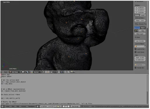
Then, it is sufficient to select the desired point and run a python script to write their coordinates to a txt file. The output is then a list on n coordinates in 3D, expressed with respect to a frame attached to Mario itself. An example of this process in Blender in 2.16.

Figure 2.16: In Blender, it is possible to select the desired keypoints (orange dots), to export them via a python script, whose editor is at the bottom. This model of Mario in Blender is indeed a mesh.

Once imported in the app, as described in 2.3.3, and the ”recenter” option is set to ”false”, Android Studio will keep that reference frame as the nominal one.

Therefore, the coordinates just extracted are the ones of the model overlapping the real object with respect to the object reference frame, making them approximations of the coordinates of the real object as well.

2.4.2 Keypoints with respect to camera

At this point, we have at our disposal a series of elements: • obj_p

i: coordinates of the i-th keypoint expressed with respect to the object reference

frame. In order to be projected on the image, we want to express all these with respect to the camera reference frame.

• world_T

obj: projective transformation matrix (4x4) of the object reference frame with

respect to the world frame, assigned by ARCore during dataset creation. It is built from the info in the file ”nodes.txt” discussed in 2.3.2.

(31)

3D pose recognition via single image based on deep networks • world_T

j−camera: projective transformation matrix (4x4) of the j-th image of the

dataset, expressing the j-th camera reference frame with respect to the world frame. This info is obtained by procesing the data in ”cameraPoses.txt” as in 2.3.2. This is the key localization structure identified by ARCore while moving the phone. With these elements, it is possible to compute the coordinates of the keypoints with respect to the camera frame by simple matrix manipulation using the following compu-tation:

j−camera_p

i = (worldTj−camera)−1∗worldTobj∗objpi (2.1)

where the ”∗” symbol is meant as a matrix multiplication operator.

After this process, considering m keypoints extracted via Blender, and n images in the dataset, we have a series of n ∗ m keypoints, m for each one of the n images, expressed with respect to their own camera reference frame.

Once plotted on the image, a series of keypoints looks like Figure 2.17, that is the drawn version of 2.12a.

Figure 2.17: This is the image from 2.12a once the extracted keypoints are drawn on it. It is noticeable how they fit well on the real object even when plotted based on the 3D model approximating it.

2.4.3 Projection on the image

Having j−camera_p

i, namely the coordinates of each keypoint with respect to the camera,

we need to teach Yolo to recognize these points on other images of the same object. In order to do so, Yolo needs to be trained with the coordinates of the keypoints on the image, namely the projection on the image plane of each j−camerapi, as well as its

label.

(32)

The label is indeed i, since we consider ordered sets of keypoints. Regarding the projection, we need to employ the projection matrix:

P =    fx 0 cx 0 fy cy 0 0 1   

where the parameters in it are taken from ”intrinsics.txt” returned by the app. In order to retrieve these values, even the standard camera calibration procedure is feasible. As a matter of fact, in order to check the validity of the values reported by the app, during the development process a camera calibration was performed and the values were found to be comparable.

The camera calibration procedure, which was done using the guide by OpenCV [14], returns also the distortion coefficients of the camera. Throughout this thesis, these coef-ficients have been considered negligible.

The coordinates in the image of each keypoint can be obtained by:    x y 1   = P ∗    pi x pi y pi z   =    fx 0 cx 0 fy cy 0 0 1   ∗    pi x pi y pi z    (2.2) It has to be noted that the result belong to the 2D projection space, and it has then 3 component. In order to have the standard 2D vector, we should divide the whole vector for the 3rd component, getting then rid of that last one afterwards.

2.4.4 Patch creation for training

Once the keypoints have been expressed with respect to the camera and projected to the image, we need to make a patch out of it, so to feed it to Yolo as something to be learned in order to recognize it on real future images.

For doing so, we use each projected keypoint as a centroid, and build around it a squared patch of a certain size.

Because of the prospective rules of pinhole camera models, an object becomes smaller as its distance from the camera increases. So, using this very concept, we should adjust the dimension of the patch built around a keypoint according to its distance from the camera, since the characteristic elements that it represents will become smaller as well. In fact, if we did not decide the patch dimensions according to the distance, we might include unwanted elements for keypoints far away from the camera.

Since from 2.4.2 we know the vectorj−camerapi, its norm represents the distance of the

i-th keypoint in the j-th image from the camera. The dimension of the patch is therefore inversely proportional to j−camerapi norm. The proportionality constant was determined

(33)

3D pose recognition via single image based on deep networks experimentally, but it can be easily adjusted.

An example of patches is in Figure 2.18.

Figure 2.18: The white squares around each yellow keypoint are patches. Notice that here the patches are all very similar in dimension since the distance to the camera for all of them is approximately the same.

To appreciate the difference in size of these patches according to distance, compare Figure 2.18 with 2.19.

Adjusting Annotations

As remarked in 4.1, it is not easy to make the 3D model of the app overlap with satisfactory accuracy to the real object during the creation of the dataset via the app.

The misalignment due to this, during this patch creation phase, would make the images with projected keypoints look like 2.20: there’s a clear gap between the intended points of interest in the image and the projected one, especially along the vertical axis.

In order to solve this problem, since this exact error propagates for all the images in the dataset, all shot with the same misaligned CAD model, it is sufficient to add to the Patch creation algorithm an additional rototranslation, which by default is set to identity therefore with no effect, which is applied to the matrix representing the pose of the object with respect to the camera.

This additional step can be adjusted manually, by looking at the effect on the repro-jected keypoints of changes along different directions (Red : X, Green:Y, Blu, Z), until satisfactory. For example, in order to fix 2.20 the additional rototranslation was set to Francesco Taurone Chapter 2 33

(34)

Figure 2.19: Here the patches are smaller in dimension with respect to 2.18 since the object is farther.

Figure 2.20: Here the effects of a misalignment of the model during App dataset creation. 34 Chapter 2 Francesco Taurone

(35)

3D pose recognition via single image based on deep networks ManualRT =       1 0 0 0 0 1 0 −0.06 0 0 1 −0.03 0 0 0 1      

meaning that there was no need to add rotations, whereas -6cm were added along the green axis and -3cm along the blue axis, resulting in 2.21.

Figure 2.21: From 2.20, by applying an additional rototranslation decided by the user, the overlapping improves significantly.

This step is important to ensure that Yolo learns to recognize the patches that the user decided, so to identify them correctly on the pose estimation pipeline. Therefore, a new file was added to each dataset, called ”manualT”, which is the specific ManualRT of that set of images, since all of them were captured for the same dataset and therefore share the same misalignment.

Moreover, this adjustment of the groundtruth makes the final evaluation of the per-formances of the pipeline more realistic, since after the correction the set of values we use as groundtruth are closer to the real ones.

(36)

(37)

Chapter 3 The final pipeline

3.1 Description

As described in the previous chapters, the final pipeline is composed of a first phase dedicated to the training of the net, and a second phase in which the real pose estimation can be retrieved. This estimation need therefore 2 separate steps, the first being yolo detection and the second the PnP Ransac reconstruction of the rototranslation from camera to object.

This chapter reports the results on these two separate components after training (3.2), then on the whole system (3.3).

A possible sequence of steps for a real use of this pipeline is summarized in the algo-rithm 1.

Result: Pose estimation

-Import the 3D model of the object in the app;

-Generate a dataset overlapping the model with the real object; -Export the desired keypoints coordinates using the 3D model;

-Generate patches around each keypoint, saving them on a training file; -Train Yolo with that dataset;

-while Camera on do

-Yolo generates bounding boxes for each image;

-The centroids of these patches are the detected keypoints; -Apply PnPRansac to retrieve the pose;

-Feed the needed pose to controller end

Algorithm 1: Proposed algorithm 37

(38)

3.2 Test of the two components

Next, the tests of the 2 main steps of the pipeline, namely Yolo detection and PnP with Ransac to get the pose, so to ensure that the performances of the 2 separately were satisfactory.

3.2.1 Datasets for testing

To test the performances of a trained deep network we need to collect sets of images that the net is supposed to understand, but that were not present in the training dataset. These are called test datasets.

The test datasets used for this thesis are:

• Dataset Close: it is made of images taken from a close distance. An example in 3.1a;

• Dataset Far: it is made of images taken from a farther distance. An example in 3.1b;

• Dataset Noisy Background: the subject of these images has various random elements as background, making the detection task more complex. An example in 3.1c; • Dataset Occlusion: the subject is partially hidden behind another object. These

make the PnP task much more challenging since elements on the object cannot be detected. An example in 3.1d.

Here the four datasets are supposed to be of increasing complexity for both the detector and the PnP pose reconstruction.

3.2.2 Test Yolo

In order to test Yolo performances, we analyze 2 parameters, Precision and Recall. These are defined as:

• Precision: given an image, precision is the ratio between two elements. The numer-ator is the number true positive results, those being the keypoints (centroids of the bounding box) that, once projected, lie within a certain distance from the ground truth projected keypoint. Conversely, the denominator is the total number of de-tected keypoint in the image, meaning the sum of true positive and false positive results. Usually, in order to evaluate the performances of a net on a whole dataset, the average of all the precisions is considered.

Precision = tp tp+ fp

(3.1) 38 Chapter 3 Francesco Taurone

(39)

(a) Image belonging to dataset close. (b) Image belonging to dataset far.

(c) Image belonging to dataset noisy back-ground.

(d) Image belonging to dataset occlusion.

Figure 3.1: Examples from the test datasets.

(40)

• Recall: given an image, recall is the ratio between the number of positively detected keypoints and the number of ground truth keypoints for that image, namely true positive summed with false negative results.

Precision = tp tp+ fp

(3.2) It has to be noted that the usual trend for these two metrics is to be in a sort of inverse proportionality.

An example of this could be made by considering the threshold above which preditions from the net are considered valid. Troughout this thesis, the threshold was set to 0.3. Consider then the possibility of increasing this threshold: what happens is that the net outputs only results with higher confidence, making the predictions more reliable and more likely to be precise. But, if on one hand the precision increases, the fact that the net now outputs only high confidence results make the recall metric decrease, since some predictions of keypoints were discarted.

Graphs and results

Following, a graph about mean precision (3.2) and mean recall (3.3) for all the 4 datasets, with various configurations of number of detectable keypoints and threshold.

The main result of this series of tests is that Yolo performs better when it is trained to recognize few keypoints. This is well shown by the negative trends of recall on all the datasets by increasing the number of detectable keypoints, meaning that among all the possible keypoints to be detected only a small percentage is recognized. This can also the highlighted by the number of images where no patch was detected by yolo 3.4. As expected, the occluded dataset shows the worst results of all, and moreover it reaches percentages above 80% for all the dataset when trained for 100 keypoints.

This is indeed a problem related to the confidence threshold Yolo uses in order to reject untrustworthy results. Since with a lot of keypoints the confidence of each detection tends to decrease, cause a patch is then similar to many others labeled differently, after a certain number of keypoints no detection is trustable anymore in the image.

It has to be noted that while the recall decreases as we train Yolo for a biggere number of keypoints, the precision is quite steady until 50kp. It means that an high percentage of the detected keypoints is close to the groundtruth, even if the ones detected are not many as highlighted by the small recall.

Moreover, looking at the different colored columns, it can be noted that after a thresh-old of 30 pixel (the green column) a further increase of the threshthresh-old doesn’t change much the corresponding precision and recall. Therefore, most of the examples in the datasets show good precision and recall at around 30 px of threshold.

An example of detection compared with the groundtruth in

(41)

Figure 3.2: Precision Mean on Yolo tests for all the datasets, with multiple thresholds (in pixels) and multiple number of keypoints.

Figure 3.3: Recall Mean on Yolo tests for all the datasets, with multiple thresholds (in pixels) and multiple number of keypoints.

Figure 3.4: Number of images where no patches where detected, representing Yolo failures. Francesco Taurone Chapter 3 41

(42)

Figure 3.5: Here the colored squares are the projected groundtruth, the colored crosses are Yolo detection’s centroids, used afterwards to calculate PNP. The

3.2.3 Test Ransac PnP

In order to test Pnp with Ransac, we feed it with the ground truth keypoints, so that it returns a pose composed of Rotation and Translation. The real algorithm will use Yolo output instead of the ground truth, since given a simple image we are not supposed to have information about the camera pose in the environment or the object pose in space. Then, we compare the estimated pose with the ground truth by means of 3 main metrics:

• Projection metric: this is very similar to precision, from 3.2.2, since it is the mean for each image of the distances in pixel of the projected keypoint and the paired ground truth one. Moreover, we keep track of the mean, standard deviation and median of the norm of the distance between computed keypoints and ground truth ones.

• Rotation metric: it checks the ”precision” for the rotation matrix, computing the norm of the error vector between the 3 angles representing the orientation of the object in space.

• Translation metric: it checks the ”precision” for the translation vector, computing the norm of the error vector between the 3 component representing the position of the object in space.

(43)

3D pose recognition via single image based on deep networks Graphs and results

The projection error mean in 3.6 is a measure of the quantity that is then analyzed with respect to a threshold for the projection metric. For this test using groundtruth keypoints, its order of magnitude is shown to be around ₁₀1 of the threshold used for the whole pipeline in 3.3, making the projection metric always 100%. Moreover, the trend in 3.6 is almost constant. This means that if the keypoints used for estimating the pose are very reliable, the number of keypoints does not seem to play a big role in the process in terms of reprojection error.

However, the results of the whole pipeline presented in the following section highlight the fact that a non minimal number of keypoints is required when those are not completely reliable, as described in 3.3.

Figure 3.6: Average projection error while testing Pnp Ransac for all the dataset varying the number of keypoints to extract the pose from.

Similarly to what happened for the pojection metric, also rotation and translation metrics showed always satisfactory results using the same thresholds as for the complete pipeline ( 3 cm for the translation error and 10 degrees for the rotation ).

Interestingly, for both rotation (3.7) and translation (3.8), an increasing number of keypoints make the error decrease. It can be noticed that after 20 keypoints, the error is approximately steady. Therefore, in order to balance the trade-off between an high number of keypoints for decreasing the Pnp Ransac error and a small number of keypoints to increase Yolo precision, 20 might be a sweet spot.

3.3 Results: Yolo and PnpRansac

In order to interpret the performances of the whole pipeline, the same metrics use in 3.2.3 will be employed, since Yolo performances are the same as for 3.2.2. The difference of this test with respect to the previous lies in what the PnP Ransac uses in order to estimate Francesco Taurone Chapter 3 43

(44)

Figure 3.7: Average error in the estimation of the orientation, while testing Pnp Ransac for all the dataset varying the number of keypoints to extract the pose from.

Figure 3.8: Average error in the estimation of the position of the object, while testing Pnp Ransac for all the dataset varying the number of keypoints to extract the pose from.

(45)

3D pose recognition via single image based on deep networks the pose. Previously, in order to test just PnP, it was fed with the groundtruth; now, with the detections from Yolo.

It has to be noted that the graphs in 3.9, 3.10 and 3.11 do not show any result for the 100kp case, since as already shown in 3.2.2 almost no detection was possible.

About the projection error in 3.9, it can be seen that, as expected, the occluded dataset is the worst of the 4 in terms of reprojection average 3.9a.

For this series of results we use the median instead of the mean, so to filter out those spurious results that highly affect the mean: the median instead represents with higher fidelity the result of the vast majority of images.

The median of the projection error is in all configurations, but for the occluded dataset, below 10 pixels.

Interestingly, the performances in terms of projection error are quite similar for the first 3 datasets. The results tend to favor farther images and few keypoints for the best projection metric. As already stated, this might be due to the decrease in precision of Yolo detections for many keypoints, as seen in 3.2.2

Looking at the rotation graphs in 3.10, we find a quite steady median of the rotation error in 3.10a around 10 degrees for the first 3 datasets. From 3.10b it can be appreciated more in detail the percentage lying below those 10 degrees threshold.

Similarly for the Translation error in 3.11, the median is quite steady for the first 3 datasets and selected number of keypoints (exception made for the occlusion dataset), around 5 cm

Interestingly, regarding the position error of the model in space, far objects are not favored, conversely to the trend for projection error. Rather, close views are the best in terms of performances.

Reprojection of the model on the images

In 3.12, examples of reprojections of the model onto images from the different dataset using the pose estimated by the pipeline.

This reprojection was achieved using Blender, by calculating the position of the camera with respect to the object. In order to do that, we need to move the camera within Blender according to the position of the camera with respect to the object, then shooting a picture at the model of the object placed in Blender at the center of the global reference frame.

In order to do so, we made use of the inverse of the matrix obtained in 2.4.2, namely:

obj_T

j−camera= (j−cameraTobj)−1 (3.3)

which represent exactly the rototranslation needed to Blender to move the camera with respect to the reference frame fixed to the object.

After that, we make use of a python script to:

(46)

(a) Median of the projection error for all the dataset with varying number of detectable keypoints.

(b) Projection metric, with threshold = 10 pixels

Figure 3.9: Projection error results for the complete pipeline, so regarding the different be-tween the reprojected keypoints according to the estimated keypoints and the reprojected groundtruth.

(47)

(a) Median of the rotation error for all the dataset with varying number of detectable keypoints.

(b) Rotation metric, with threshold = 10 degrees

Figure 3.10: Rotation error results for the complete pipeline, so regarding the difference in degrees between the estimated orientation and the grondtruth.

(48)

(a) Median of the translation error for all the dataset with varying number of detectable keypoints.

(b) Translation metric, with threshold = 3 cm

Figure 3.11: Translation error results for the complete pipeline, so regarding the difference in cm between the estimated position of the object in space and the groundtruth.

(49)

(a) Reprojection on image belonging to dataset close.

(b) Reprojection on image belonging to dataset far.

(c) Reprojection on image belonging to dataset noisy background.

(d) Reprojection on image belonging to dataset occlusion.

Figure 3.12: Reprojections on images from the test datasets. The grey shadow represents the predicted pose of the object in space.

1. Move the camera to the desired position, which is the pose of the camera of the j-th image;

2. Shoot a picture with no background of the model imported in Blender; 3. Reduce its opacity, and overlay it to the j-th image of the dataset.

In this way it is possible to visually appreciate the performances of the pose estimation. Sided object correlation with errors

Since a considerable standard deviation was highlighted in all the tests results, we try to investigate the reasons for that.

Visually, when looking at the results of the pose estimation for the different datasets, we notice that errors seem to be more frequent with sided images, those being images where the object is oriented side-wise rather then front-wise.

(50)

In order to deepen our understanding of this phenomenon, namely to see if there is a real correlation between sided images and errors spikes, we need to calculate how sided each image is.

The technique for achieving this measurement is a cross product between the axis of the camera facing the object and the z axis of the object, which points to the front part of it. This is possible since we have for each image in the dataset the initial position of object with respect to the world, and the position of the camera with respect to the world for each image.

Therefore, similarly to what is done in 2.4.2:

j−camera_T

obj = (worldTj−camera)−1∗worldTobj (3.4)

In order to do the cross product between the z axis of the object and the frontal (x) axis of the camera, we do:

side = h 1 0 0 0 ij−camera Tobj ∗       0 0 1 0       (3.5) which is indeed the component of the first row and third column of the matrix. Therefore, a side value of 0 corresponds to a perfectly frontal object, whereas 1 cor-responds to the camera facing the right side of the object, -1 facing its left side. The correlation is calculated with respect to the absolute value of this side measurement, since we just want to highlight that the object is on the side, regardless of which one.

The graph in 3.13 shows the mean correlation of this ”side” measure with Projection error, Rotation Error and Translation Error. The correlation is a number from −1 to 1, where the higher the absolute number of the value, the higher the correlation.

Figure 3.13: Correlation between how on the ”side” is the subject of the image and the metrics used for judging the pose estimation. This correlation uses the absolute value of the ”side” as variable, since we don’t care which side the object is but just that it is sided. 50 Chapter 3 Francesco Taurone

(51)

3D pose recognition via single image based on deep networks It is indeed a non-zero correlation most of the times, meaning that indeed being on the side affects the errors of the pose.

A possible reason for that might be that a good portion of objects has key features on the front and back face, meaning that users are more likely to select keypoints along those two ”planes”. When the camera is looking at the object laterally, it is possible that many of those keypoints overlap, making the detection process by Yolo more difficult, which would result in less precise estimations of the pose as well.

It has to be highlighted that if on one hand, for close and far images mainly, the correlation is positive, meaning that if the position is more on the side the error increases, on the other hand for Noisy background and occlusion the correlation is negative.

This could be due to the fact that for these 2 dataset a sided image might correspond to a better detection of the keypoints that before were hidden or placed in front of a noisy background, improving the performances of the detection.

3.3.1 Training with multiple objects

For the applications described in the previous chapters, it would be advisable to have a system able to recognize the pose of multiple kinds of objects in the surrounding environ-ment. Up to now, this thesis focused only on the recognition of a single kind of object, namely ”Mario”, as primary subject of the tests, whereas this section reports the result of this pipeline trained for multiple objects.

We test the case of 2 objects, Mario and a Bunny shaped toy, assuming that only one of the two is present in the scene at a time. The presence and recognition of multiple objects in the scene is suggested as further development in 4.1.

The steps followed for generalizing the 1 object pipeline to a 2 or more object pipeline are:

1. Make a 3D model for the new objects, and extract/measure the local coordinates of the keypoints needed for making the datasets;

2. Import these new models to the app, so to be able to place it in the environment as AR object;

3. Make a new set of datasets for each new object, one for training Yolo and four (close, far, noisy background and occlusion) for testing the results (if needed);

4. Retrain Yolo, making sure to differentiate the labels for each object. As a matter of fact, two objects should not share any label. As example, if it’s planned to detect 7 keypoints on 2 objects, an advisable choice is that the labels go from 0 to 6 for the first and from 7 to 13 for the second;

5. Select the newly trained Yolo for detecting the keypoints needed by PnP.

(52)

After these steps, Yolo is trained to recognize all those objects in the scene. Graphs and results

The results with Yolo trained for more then 1 object are satisfactory. It is noticeable indeed that the performances of this setup are quite comparable with the one trained for a single object. Meaning that Yolo is perfectly capable of learning a multitude of object precisely enough that this pipeline is robust nonetheless.

Following is the series of graphs about whole pipeline performances already explained in the previous section, here reported for comparing the results. As highlighted previously, this setup take as assumption the presence of a single object at a time in each image.

It is interesting to notice that for the occluded dataset, having an higher number of object for the yolo training improves its performances on the complete pipeline.

(53)

(a) Median of the projection error for all the dataset with varying number of detectable keypoints. The version for single object in 3.9a.

(b) Projection metric, with threshold = 10 pixels. The version for single object in 3.9b.

Figure 3.14: Projection error results for the complete multi-object pipeline, so regarding the different between the reprojected keypoints according to the estimated keypoints and the reprojected groundtruth. The version for single object in 3.9.

(54)

(a) Median of the rotation error for all the dataset with varying number of detectable keypoints. The version for single object in 3.10a.

(b) Rotation metric, with threshold = 10 degrees. The version for single object in 3.10b.

Figure 3.15: Rotation error results for the complete multi-object pipeline, so regarding the difference in degrees between the estimated orientation and the grondtruth. The version for single object in 3.10.

(55)

(a) Median of the translation error for all the dataset with varying number of detectable keypoints. The version for single object in 3.11a.

(b) Translation metric, with threshold = 3 cm. The version for single object in 3.11b.

Figure 3.16: Translation error results for the complete multi-object pipeline, so regard-ing the difference in cm between the estimated position of the object in space and the groundtruth. The version for single object in 3.11.

(56)

(57)

Chapter 4 Conclusions

The results of this pipeline are quite satisfactory, for both single object training and multiple. Few key considerations are worth noticing, among many pros and cons for this solution.

PROS:

1. Given the performances in terms of pose estimation, this pipeline is suitable for application where no highly precise results are needed. Nonetheless, the results are quite satisfactory, and is well suited for a wide variety of application (like non fragile object grasping or AR visualization).

2. In order to build this pipeline from scratch for a given application, just few hours are required. As a matter of fact, for a set of few objects, Yolo is relatively quick to train and the creation of the needed datasets is sped up thanks to the semi-automatic creation via App.

3. The process of adding a new object to the recognizable ones is fairly easy and quick, since it requires its 3D model for the app and a new dataset fort the training. CONS:

1. The need of a CAD model is inconvenient, since it is not always available. However, especially for industrial application, it is a reasonable requirement. One could avoid the use of CAD models by measuring the keypoints and placing a cube in the app to retrieve the position of the object, at the expenses of accuracy.

2. During dataset creation via App, it is not always easy to place the model in the environment as precisely as intended. In fact, it is for this reason that a manual refinement step has been added for a more precise dataset and consequently a better training.

Moreover, it is unlikely to measure the real performances of the algorithm, since the groundtruth itself is extracted from the model placed in the app which is noisy.

(58)

4.1 Further developments

During the development of this thesis, it was possible to highlight multiple possible im-provements for the current implementation. The most relevant ones are:

• Being able to detect multiple objects form the same scene. It is indeed quite easy to achieve given the current configuration, just forcing PnP to consider only detection labeled for the same object, repeating the process for all the objects in the scene. • Automatic selection of good keypoints for this task. It could be useful to find a

way to train a network to recognize, given an object, which keypoints would be the best for a pose estimation task. For the current implementation, this is just a user choice.

• Try with a more specialized Deep Network, different from Yolo, to compare the performances.

• Make the process of overlapping the 3D model on the app with the real world object on the screen an easier task. Right now, one of the causes of the errors metrics shown before was cause by a misalignment between the 2, which add an error to the groundtruth used to judge the results.

• Fine tuning of parameters: since some are key elements of the algorithm, like the patch size and the adjustment based on the distance of the model, it would be worth it to test more in depth the changes in performance according to modifications in those parameters.

• On each image of each dataset, all the nominal keypoints are plotted and saved as annotation to be learnt by Yolo. This happens also for those keypoints that are ”hidden” by objects in the image, so that for example the tail of the bunny is written as patch even when the bunny is in front view. It would be interesting to implement a sort of hiding process making use of the groundtruth, so that all the keypoints whose reprojection line intersects the model is discarded. This might improve Yolo’s accuracy, and therefore the performances of the whole pipeline.

3D Object Recognition from a Single Image via Patch Detection by a Deep CNN

ALMA MATER STUDIORUM

UNIVERSITY OF BOLOGNA

3D Object Recognition from a Single Image via Patch Detection

by a Deep CNN

Contents

Introduction

Abstract

Chapter 1

Pose Recognition - State of the art

1.1

Examples of successful algorithms for 3D Pose

Estimation

Chapter 2

Development of the algorithm

2.1

Choice of the network

2.1.1

What is Yolo

2.2

Prototyping with a simple object - the raspberry

box

2.3

The App to create datasets

2.3.1

ARCore and its use

2.3.2

The use of the app

2.3.3

Issues and solutions

2.4

3D models and keypoints identifications

2.4.1

Blender - keypoints extraction with respect to the object

2.4.2

Keypoints with respect to camera

2.4.3

Projection on the image

2.4.4

Patch creation for training

Chapter 3

The final pipeline

3.1

Description

3.2

Test of the two components

3.2.1

Datasets for testing

3.2.2

Test Yolo

3.2.3

Test Ransac PnP

3.3

Results: Yolo and PnpRansac

3.3.1

Training with multiple objects

Chapter 4

Conclusions

4.1

Further developments