FACULTY OF ENGINEERING
INTERNATIONAL MASTER COURSE IN CIVIL ENGINEERING
D I C A M
Civil, Environmental and Materials Engineering
THESIS IN
Advanced Design of Structures
TIME-DEPENDENT BEHAVIOUR OF
REINFORCED CONCRETE SLABS
CANDIDATE SUPERVISOR
Stefano De Vittorio Chiar.mo Prof. Marco Savoia
Chiar.mo Prof Gianluca Ranzi
COSUPERVISOR
Chiar.mo Prof. Claudio Mazzotti
Academic Year 2010 – 2011 Session III
FACULTY OF ENGINEERING
MASTER DEGREE IN CIVIL ENGINEERING
School of Civil Engineering
EXCHANGE STUDENT PROGRAM
TIME-DEPENDENT BEHAVIOUR OF
REINFORCED CONCRETE SLABS
CANDIDATE SUPERVISOR
Stefano De Vittorio Chiar.mo Prof. Marco Savoia
Chiar.mo Prof Gianluca Ranzi
COSUPERVISOR
Chiar.mo Prof. Claudio Mazzotti
III
Abstract
In this thesis is studied the long-term behaviour of steel reinforced slabs paying particular attention to the effects due to shrinkage and creep. Despite the universal popularity of using this kind of slabs for simply construction floors, the major world codes focus their attention in a design based on the ultimate limit state, restraining the exercise limit state to a simply verification after the design. For Australia, on the contrary, this is not true. In fact, since this country is not subjected to seismic effects, the main concern is related to the long-term behaviour of the structure.
Even if there are a lot of studies about long-term effects of shrinkage and creep, up to date, there are not so many studies concerning the behaviour of slabs with a cracked cross section and how shrinkage and creep influence it. For this reason, a series of ten full scale reinforced slabs was prepared and monitored under laboratory conditions to investigate this behaviour. A wide range of situations is studied in order to cover as many cases as possible, as for example the use of a fog room able to reproduce an environment of 100% humidity.
The results show how there is a huge difference in terms of deflections between the case of slabs which are subjected to both shrinkage and creep effects soon after the partial cracking of the cross section, and the case of slabs which have already experienced shrinkage effects for several weeks, when the section has not still cracked, and creep effects only after the cracking.
1
Table of Contents
ABSTRACT... III TABLE OF CONTENTS ... 1 CHAPTER 1 ... 5 INTRODUCTION ... 5 1.1 Background ... 61.2 Aims and objectives ... 8
1.3 Layout of the thesis ... 9
1.4 Literature review ... 10
1.4.1 Introduction ... 10
1.4.2 Deflections ... 10
1.4.2.1 Computation of deflections... 12
CHAPTER 2 ... 15
TIME-DEPENDENT BEHAVIOUR OF CONCRETE ... 15
2.1 Overview ... 16 2.2 Creep ... 17 2.3 Shrinkage ... 18 CHAPTER 3 ... 21 THEORETICAL MODEL ... 21 3.1 Introduction... 22 3.2 Theoretical methodology ... 22
3.2.1 Cross Sectional Analysis (CSA) ... 22
3.2.2 Time-dependent behaviour of concrete ... 23
3.2.2.1 Constant and non uniform shrinkage deformations ... 23
3.2.2.2 Principle of superposition - the Step-by-Step Method (SSM)... 25
2
3.3 Detailed expressions of the numerical formulation for a cracked section ... 26
3.3.1 Age-adjusted Effective Modulus Method ... 27
3.3.1.1 Short-term analysis ... 27
3.3.1.2 Long-term analysis ... 31
3.3.2 Step-by-Step Method ... 34
3.4 Derivation of the deflection of a supported beam for which the curvatures at the supports and at the mid span are known ... 39
CHAPTER 4 ... 43
VALIDATION OF THE NUMERICAL MODELS: COMPARISON WITH PREVIOUS EXPERIMENTAL MEASUREMENTS ... 43
4.1 Description of the previous experimental test ... 44
4.2 Validation of the models: comparison of the results ... 47
CHAPTER 5 ... 51
EXPERIMENTAL PROGRAM ... 51
5.1 Overview ... 52
5.2 Specimens description ... 52
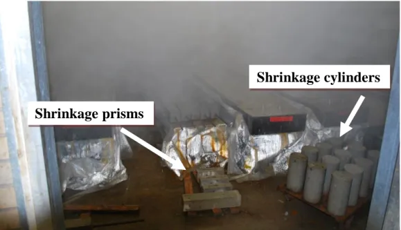
5.2.1 Shrinkage and creep samples ... 53
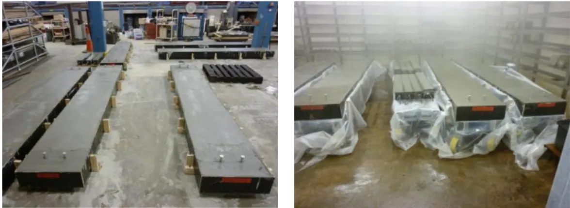
5.2.2 Simply supported slabs ... 56
5.2.2.1 General description ... 56
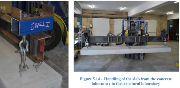
5.2.2.2 Lifting anchors ... 57
5.2.3 Loads ... 58
5.2.3.1 Design procedure of the load used in the test ... 59
5.3 Experimental procedure ... 63
5.3.1 Shrinkage samples and creep rig ... 63
5.3.2 Simply –supported slabs ... 63
5.4 Instrumentation ... 64
5.4.1 Measurement devices... 65
5.4.1.1 Demec targets ... 65
5.4.1.2 Strain Gauges Transducers ... 66
5.4.1.3 Strain gauges ... 67
5.4.1.4 PI transducers ... 68
5.4.1.5 Data logger ... 69
3
CHAPTER 6 ... 71
SHRINKAGE AND CREEP RESULTS, EXPERIMENTAL TEST AND INSTANTANEOUS AND LONG-TERM RESULTS ... 71
6.1 Shrinkage result ... 72
6.1.1 Before the experimental test ... 72
6.1.2 After the experimental test ... 77
6.2 Creep result ... 79
6.3 Experimental test ... 82
6.4 Instantaneous results ... 84
6.5 Long-term results ... 88
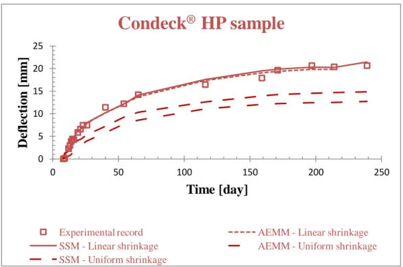
6.5.1 Mid span deflection ... 89
6.5.2 Strain in the steel bar ... 91
6.5.3 Top and bottom displacement ... 93
CHAPTER 7 ... 97
COMPARISON BETWEEN EXPERIMENTAL AND ANALYTICAL DEFLECTIONS ... 97
7.1 Introduction... 98
7.2 “Dry” samples comparison ... 98
7.3 “Fog” samples comparison ... 103
CHAPTER 8 ... 107
CONCLUSIONS ... 107
ACKNOWLEDGMENTS ... 111
REFERENCES... 113
APPENDICES ... 117
APPENDIX A - DRAWINGS OF THE SLABS AND OF THE INSTRUMENTATION... 119
A.1 Handling of the slabs ... 119
A.2 Experimental test scheme to crack the slabs ... 119
A.3 Slabs with the sustained loads applied after the cracking test ... 120
A.4 Instrumentation ... 121
4
APPENDIX C - PHOTOS OF THE EXPERIMENT ... 131
C.1 Before the pour ... 131
C.2 Poured slab and curing ... 132
C.3 After curing, before cracking test ... 133
C.4 Movement of the slabs ... 133
C.5 Data logger setup ... 134
C.6 Test: phase 1... 135
C.7 Test: phase 2... 136
5
Chapter 1
Introduction
“Engineering is a great profession. There is the
satisfaction of watching a figment of the imagination emerge
through the aid of science to a plan on paper. Then it moves to realisation in stone or metal or energy. Then it brings homes to men or women. Then it elevates the standard of living and adds to the comforts of life. This is the engineer's high privilege.”
6
1.1
Background
The construction techniques and the materials used for building are constantly improving in the last years, but concrete and steel remain the two main ingredients to build any kind of civil construction. They are the best ones, up to now, to provide, respectively, the required resistance in compression and in tension.
A structure is usually designed based on the ultimate limit state requirements given by the national building code of practice. These requirements are relative to the strength of the structure, i.e. the ability of the structure to carry the design ultimate loads without collapsing. But these are not the unique requirements that a structure must satisfy. There are also the so called serviceability limit states. Serviceability requirements refer to the behaviour of structures at working loads and they are satisfied when the structure does not deflect or crack more than certain limits provided by the building codes. Both cracking and deflection are primarily dependent on the properties and behaviour of the concrete, but are more difficult to predict because of the non-linear, inelastic and time-dependent nature of the concrete. In this thesis, the attention is focused on the serviceability issues related to the time-dependency nature of concrete and thus on shrinkage and creep effects and their fundamental role in the design procedure. In this view, the long-term effects of the materials composing the structure become a critical factor which must be taken into account in the design procedure.
The aim of the serviceability limit state is to provide an indication about the admissible deflection that a concrete structure can support over a period of time. Design a structure which complies with these limits is a considerable challenge for a structural engineer, since the properties of concrete, without any doubt the most common construction material in the world, are not predictable with certainty. The uncertainties related to the long-term behaviour of concrete are mostly related to its propensity to crack under tensile stresses and to the predictability of time-dependent properties that characterize it. Gilbert (1), in one of his numerous publications regarding the topic, refers that the serviceability failure of a structure in Australia is quite common, even if most of these structures satisfy the requirements provided by the relevant code of practice.
Nowadays concrete structures are becoming always more elaborated, due to the higher architectonical complexity and due to the developed construction
7 techniques involved. Always more often, a structure is a combination of conventional reinforced concrete, post tensioning or composite member and so on. In this view, appears evident the necessity to have a better understanding of the main concrete properties and their influence on the general behaviour. This is extremely valid for time-dependent comportment. As a matter of facts, creep and shrinkage, the time-dependent characteristics of concrete, are really uncertainty to quantify. Always Gilbert (1) believes that shrinkage is the most problematic factor to be determined. In addition, in this project, the presence of a cracked cross section should not be forgotten, because it influence decisively all the other factors.
How creep and shrinkage develop in time is quite difficult to be predicted and quantified, since they verify as rather chaotic event. Usually shrinkage of concrete is mainly caused by the evaporation of moisture from the concrete to the outside environment (drying shrinkage); the consequence is a reduction of the concrete volume if there are no restrains, or, in presence of it, the consequence will be a change in the build-up of stresses. Creep starts only after the application of a load on the specimen, and thus, many times, the main difficulty is to differentiate it from the shrinkage component, since experimental measurements take into consideration both of them together.
Several parameters influence the development of creep and shrinkage. Just to name a few of them, let’s consider the specimen condition of exposure and the environmental conditions themselves (e.g. temperature and relative humidity). For example, the sealing condition of the sample can strongly influence how long-term effects develop. Usually building codes, as the Australian Standards (2) or the Eurocode (3), do not take into consideration this, and therefore, the actual results can be significantly different from the theoretical ones.
In this test, in addition to long-term effects, there are some more uncertainties in the general behaviour related to the presence of a cross section partially cracked. As this study will demonstrate, the final deflection is considerably affected by these openings.
This thesis presents an original study on the behaviour of reinforced slabs under service loading conditions. The project involved the preparation of a series of full scale reinforced slabs and the fundamental factors affecting the long-term behaviour of these structures were identified and studied. The results have shown
8
that shrinkage and creep are the main factors affecting the long-term behaviour of such structures and that the cracked cross section plays a fundamental role in the final deflection value.
1.2
Aims and objectives
The main task of this project is to investigate the time-dependent comportment of reinforced concrete slabs. Particular attention is paid to understand how creep and shrinkage behave and develop in the case of a partially cracked cross section. The aim is to improve the serviceability design of these reinforced concrete slabs.
Furthermore a theoretical model is developed to account for the concrete time-dependent behaviour when dealing with building floors. The adequacy of the proposed model for the long-term prediction of reinforced concrete slabs must be evaluated as additional aim of the project. To finalize this objective, a numerical comparison is developed with a previous test on composite post-tensioned slab.
The role that a crack has in regard to creep and shrinkage is one of the key points that this test wants to investigate. The crack modifies the tensile concrete reacting part and consequently it modifies the distribution of stresses between steel and concrete. In addition, different values of loads are used to investigate more deeply which is the contribution of creep and how it influences the overall comportment. Furthermore, regarding shrinkage, part of the slabs prepared are stored in a “fog room”, a constant 100% relative humidity room, to avoid that shrinkage start before than creep. For these samples, the long-term effects develop simultaneously starting from the cracking operation day.
Since the analytical models provided by the standards for the calculation of creep and shrinkage can be misleading and since they differ quite a lot from the actual case studied, this projects is based on experimental measures of these two effects. It is a quite time-consuming work, but it allows for the use of exact parameters, the best ones that can fit the problem. In addition, in this way, it can be obtained some laboratory controlled data to calibrate, validate and extent analytical models that are being developed concurrently with the experimental program.
In order to achieve these objectives, the work has been subdivided into a number of discrete tasks which are summarized as follow:
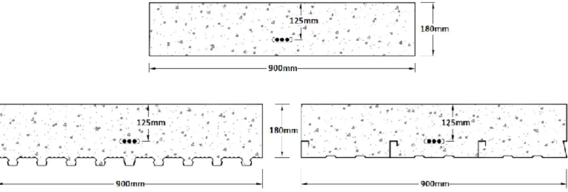
9 Six fully-supported slab specimens with two different reinforcement layouts were casted, cured for a period of 8 days and then monitored, through the use prismatic and cylindrical samples subjected to the same environmental condition, for a period of about 60 days to measure the effects of drying shrinkage.
Four fully supported slab specimens with a single reinforcement layout were casted and stored in a “fog room”, to avoid shrinkage effects. Also in this case a monitoring process was held with the use of prismatic and cylindrical samples for a period of about 60 days.
After this initial period all the ten specimens were partially cracked and then subjected to three different load conditions. The effects of varying the quantity of reinforcing steel, the bar spacing and the load conditions were studied.
Two analytical models were developed and used to study the creep and shrinkage effects. In addition, these models were also validated through the comparison with a previous experimental test performed some time before in the same University of Sydney.
A series of test were also conducted to obtain the creep and shrinkage characteristics of the concrete, and other properties such as compressive strength, tensile strength and elastic modulus, to provide accurate data for analyzing the specimens
1.3
Layout of the thesis
The thesis is structured in seven chapters and three appendices. An Introduction and the literature review of previous work published in the open literature is presented in Chapter 1. The fundamental concepts related to the time-dependent behaviour of the concrete are outlined in Chapter 2. This is followed, in Chapter 3, by the description of the theoretical model able to predict the time-dependent behaviour of the reinforced concrete and composite steel-concrete members. In addition, this chapter presents how to calculate the deflections at the mid span once the curvature is known at the two supports and at the mid span of a simply-supported slab. The ability of the proposed theoretical approach to predict the long-term response of composite post-tensioned slabs is outlined in Chapter 4 using experimental results recently collected at the University of Sydney. Chapter 5 presents the complete experimental program. It explains in detail the description of the specimen, the experimental procedure and the instrumentation used. It also contains the design
10
procedure adopted to decide the dimension of the load blocks used in the sustained load phase. Chapter 6 contains the experimental test results and a brief discussion on what obtained. More in detail, a comparison between experimental and numerical results is held in order to determine how much they differ among them. Finally, Chapter 7 presents the conclusions and gives general recommendations regarding the serviceability design of steel reinforced concrete slabs.
APPENDIX A contains more detailed and complete drawings related to the test. APPENDIX B contains a detailed explanation of the procedure used for the installation of the strain gauges on the steel bars. In the end, in APPENDIX C, there are some photos regarding the test.
1.4
Literature review
1.4.1 Introduction
The comportment of structures at service load is a fundamental design consideration. If a slab system is designed according to the strength requirements, the degree of safety against collapse may be adequate, but the performance at service loads may be not. For this reason, the design procedure should follow three main concepts and satisfy them: strength at overloads, deflections at service loads and crack widths at service loads. The aim of designing must be to ensure an adequate margin of safety against collapse and against the possibility that the structure becomes unsatisfactory for use at service loads.
The Eurocode (3) and the ACI Code (4) emphasize a design based on the ultimate limit state (strength) with additional checks on the exercise limit state. Deflections are controlled imposing a maximum admissible limit value, or alternatively, specifying a minimum allowable slab thickness in order to ensure an adequate stiffness. Regarding cracking in one-way slabs, the design should be revised in the case of reinforcement yield strength larger than 300 N/mm2.
1.4.2 Deflections
The deflection prediction is a challenge in case of reinforced concrete structures and it is even more problematic for slabs. Two main problems are related to this prediction. The first is to find a function able to describe the deflection, as the familiar wl4 384EI used for prismatic beam of span l
11 with fixed ends carrying a uniform load per unit length w . The second is to determinate the appropriate flexural rigidity EI to use in the deflection function, once it has been found.
The elastic theory analysis of a slab is quite complicated, but the availability in the last ten years of always more powerful computers and softwares based on finite element analysis is easing the problem to some extent. Considering also that the deflection functions have been calculated and tabulated for many cases, the more serious problem is nowadays related to the calculation of the flexural rigidity EI . The determination of this quantity is more difficult for a slab than a beam, largely because the reinforcement ratios in slabs are usually quite slow, due to relative low bending moment. Quite often the reinforcement ratio is governed by maximum bar spacing or minimum steel area requirements. A direct consequence of the low steel ratios is a large value of the ratio between uncracked and cracked flexural rigidity EIg EI ; thus also cracking amount has cr an influence on the deflection.
Assuming, as it is in reality, a spreading of cracking with time, the long-term deflections may be larger than the initial ones. According to the ACI Code (4), if there is no compression steel, the total long-term deflection is 3 times the initial deflection. But a series of experimental tests demonstrates that this provision may be unsafe in some cases. For example, Taylor and Heiman (5) (6) reported long-term experimental results on flat slabs which, after 2.3 years from loading, the time-dependent deflections were about 6.5-7.5 greater than the initial ones.
It is also challenging to define acceptable deflections. The last ones depend on the use of the structure and the nature of the other components, structural and no structural, of the building. Excessive deflections interfere with the function of some non-structural components. For example, if the floor deflects too much, rigid masonry walls may crack and doors and windows may no longer fit properly.
Blakey (7) studied the deflection of flat plate structures and suggested that if cracking of masonry partitions is to be avoided, initial deflections may have to be limited to about span/1500. In addition, he suggested that the minimum plate thickness should be span/32, using, as reference span, the long-span center to center of columns.
12
long-term excessive deflection. Thus it is important to reduce it as much as possible. Shrinkage strain is sometimes also responsible for cracking after the completion of the slab. In turn, shrinkage is restrained by the reinforcement in the concrete and also by other elements in the structure such as beams, columns and walls. The tensile stress caused by the restraint of the shrinkage strains, combined with the stresses caused by loads, may produce some cracks at a lower load level than otherwise expected. For this reason, any measure that reduces the shrinkage is a benefit in maintaining deflections as lower as possible.
1.4.2.1 Computation of deflections
A common deflection expression is expressed in the form
4 4 1 1 1 3 wl wl C C D Eh (1.1)
where w is the uniformly distributed load per unit area; C and C are 1 constants depending on the panel shape, support conditions, and Poisson’s ratio;
1
l the long span, either as clear span, center-to-center span or some average span;
3 2
12 1
DEh , the slab stiffness per unit width; E the Young’s modulus; and h the slab thickness. For the same reasons mentioned above, there are significant difficulties in determining the values of C and C for the 1 uncertainty related to the realistic support conditions, and in determining the effective value of D when time-dependent effects and cracking must be taken into account.
The most comprehensive studies of deflections of reinforced concrete slabs structures available are those by Vanderbilt et al, (8) and (9), Chang and Hwang, (10) and (11), and Jofriet (12).
The work done by Vanderbilt and Chang and Hwang is directed to the general problem of slabs with and without beams, while Jofriet’s concerns flat plate structures that may have spandrel beams. All considered both the effects of cracking and the elastic theory analysis for deflections. The elastic theory deflection values are considered first.
Vanderbilt’s work can be summarized as an extensive table of elastic deflection coefficients, the ones reported as C in equation (1.1), for typical interior panels supported on square columns considering the beam relative
13 stiffnesses, support size and panel shape. Chang and Hwang (10) analysed a group of slabs similar to the Vanderbilt’s ones, but using the finite element method. The deflection results match quite perfectly for similar slabs. In a second moment, they extend the formulation to take into account cracking and the different restraint conditions existing in the ends span and successively they altered it to account for creep effects. Their formulation for short-term deflection is 4 1 n s a b c wl K K K D (1.2)
where K is the elastic deflection coefficient, a K the coefficient accounting b for the state of cracking, K the coefficient accounting for reduced restraint in an c end span, and l the clear span in the long-span direction. Each of the K values n1 derives from a semi empirical formulation. To take into consideration long-term deflections, the applied load w is substituted by
wviws
, where w is the vvariable part of the load that is assumed to cause no creep, w the sustained load s consisting of the self-weight plus the sustained part of the live load, and i 1 , where is a creep multiplier.
According to Jofriet’s research (12), the mid span deflection of a typical interior panel of a beamless slab is
4 max 3 i l i wl C Eh (1.3)
where C is a coefficient depending on the support shape and panel shape, E i the concrete modulus of elasticity, h the slab thickness, w the uniformly distributed load per unit area, and l a weighted average of the long clear span l l n and the long center-to-center span l , where
3 4 n l l l l (1.4) 3 0.0285 0.0375 s i l l C l (1.5)
The short-span l is also a weighted average. The results obtained through s these equations do not match exactly with the Vanderbilt’s ones, but they are
14
sufficiently close. This is due to the fact that the results were obtained from a study of deflection computed by finite element and other solution of slabs.
Elastic deflection coefficients for additional cases are given by Timoshenko and WoinoWsky-Krieger (13) and by Brotchie and Wynn (14).
Regarding the choice of the flexural rigidity, Vanderbilt et al (8) (9) suggested two empirical approaches. In the case of low loads, up to the one causing the initial mid span cracks, deflections should be computed with the gross flexural rigidity EI . For higher values of load, the suggestion is to use the fully cracked section value EI . In addition, for intermediate loads, two different transitions cr were suggested to compute deflection. These transitions are based on the observed load-deflection curves. Jofriet (12), instead, suggested a simple equation providing a reduction in stiffness as the moment exceeded the cracking moments.
15
Chapter 2
Time-dependent behaviour of
concrete
“Research is what I'm doing when I don't know what I'm doing.”
16
2.1
Overview
When a concrete member is subjected to a sustained applied load it undergoes an instantaneous deformation at the time of loading followed by a time-dependent one over time. In most of the cases, the time-time-dependent component is greater than the instantaneous one. This behaviour of the concrete should be considered in the checks related to serviceability limit state. Under the hypothesis of constant stress and temperature, the time-dependent response is due to the creep and the shrinkage of the concrete.
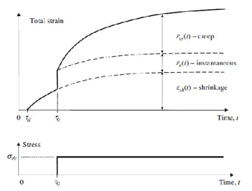
The total strain developed by concrete over time can be defined as the sum of an instantaneous strain, a creep strain, a shrinkage strain and a temperature strain. Assuming a constant temperature, the total strain results:
t e
t cr
t sh
t
(2.1) As represented in Figure 2.1, the shrinkage component does not depend on the load history, while, the other two depend on the applied stress. Shrinkage starts soon after the concrete has been poured, as the latter begins to harden, while creep occurs when the concrete is subjected to an sustained load.
Figure 2.1 – Concrete strain components in a specimen subjected to a sustained load (15) Creep and shrinkage tend to increase with a decreasing rate over time. As suggested by Gilbert (15), about 50% of the final creep develops in the first 2-3 months and about 90% after 2-3 years. Similarly, 30% of the final shrinkage is developed in the first 2-3 weeks.
17
2.2
Creep
As defined in (16), in materials science, creep is the tendency of a solid material to slowly move or deform permanently under the influence of stresses. It occurs as a result of long-term exposure to high levels of stress that are below the yield strength of the material. Creep is more severe in materials that are subjected to heat for long periods, and near melting point. Creep always increases with temperature.
Creep of concrete develops in the cement paste, after its hardening; this paste is composed by a cement gel and a series of included capillaries, and it is made of colloidal sheets formed by calcium silicate hydrates and evaporable water. The mechanism through which creep occurs has always been a cause of controversy among the scientific community and until now there is not a satisfactory theory able to describe the formation of creep. Bazant (17) explains that it is generally believed that creep is due to the disorder and instability that characterize the bond between the colloidal sheets.
Creep is affected by numerous factors which include, among the others, concrete mix, environmental and loading conditions. Generally, for increasing concrete strength, the concrete capacity to creep decreases. In addition, the creep capacity decreases for either an increasing maximum aggregate size or aggregate content and for a reduction of water/cement ratio. As previously mentioned, creep is also influenced by environment: it increases in thin members with large surface-area-to-volume ratios, such as slabs, and it also increases for reducing humidity and increasing temperature. Finally, creep depends on the magnitude and duration of the stress and on the age of the concrete at which the stress was applied for the first time. In particular, concrete creeps more when loaded at an early stage.
Usually, creep strain is formed by two main components: recoverable creep and irrecoverable creep. When subjected to a sustained stress0, creep increases at a decreasing rate. Removing this load at a time1, creep tends to decrease gradually, as reported in Figure 2.2. At this time, a sudden change in the total strain occurs, due to the elimination of the instantaneous strain. Thus, a smaller part of the creep strain is recoverable, while a bigger part of it is irrecoverable.
18
Figure 2.2 – Recoverable and irrecoverable creep components. (15)
During the last century, several analytical methods were developed to take creep into consideration. Most of them are based on the calculation of the creep coefficient, defined as the ratio of the creep deformation over the instantaneous one. It quantifies the capacity of concrete to creep. The simplest analytical method available to account for creep is Faber’s Effective Modulus Method (EMM) (18). The basic idea of this model is to modify the elastic modulus of the concrete to account for creep. A slightly more complex model is the Age-adjusted Effective Modulus Method (AEMM). A more refined model is represented by the Step by Step Model (SSM) which enables a more accurate prediction of the changes in the concrete stresses taking place over time.
2.3
Shrinkage
Shrinkage is commonly defined as the time-dependent change in volume of a non-stressed concrete specimen at constant temperature and it affects every concrete structure during its service life.
Shrinkage is larger on the external surface of a member, i.e. the one exposed to drying, while it decreases when moving towards its inner part. Figure 2.3a depicts the shrinkage distribution through the thickness of the cross section in which sh is the mean shrinkage strain value. sh is the strain required to restore the compatibility, and thus the hypothesis of plane section. A typical distribution of the instantaneous and creep strain distributions are shown in Figure 2.3b and this is equal and opposite to sh. Based on this, the total strain caused by shrinkage, obtained from the sum of elastic, creep and shrinkage components, is linear, as shown in Figure 2.3c. In this way compatibility is
19 satisfied.
Figure 2.3 – Strain components caused by shrinkage in plain concrete (15)
For a specimen with the complete perimeter exposed to air, the shrinkage deformation in it longitudinal direction can be defined as
0 0 0 , i sh i l l l (2.2)where l0 represents the initial longitudinal length at time t0 and li the longitudinal length after shrinkage has developed at ti.
For typical structural engineering applications, the design values of shrinkage deformations is of the order of 500 – 800 microstrains.
When concrete is exposed to air it tends to shrink, while, when it is subjected to water, it tends to swells (19). When shrinkage or swelling is restrained some stresses develop. In reinforced concrete structures, examples of restrain are the supports or the reinforcing bars. Usually, in concrete members, the shrinkage effects are larger in absolute value than the swelling effects and they verify frequently. For this reasons, in most of the analysis, only shrinkage effects are taken into consideration, even if the analytical procedure is exactly the same, except for the sign of the term representing the amount of volume change.
Usually, shrinkage is divided into four components: plastic shrinkage, chemical shrinkage, thermal shrinkage and drying shrinkage. Plastic shrinkage develops before the concrete has hardened and is associated with the evaporation of the surface water of the mix. Thermal shrinkage is a consequence of the heat induced during the hydration process and does not last more than a few days. Chemical shrinkage (or autogenous shrinkage) is caused by the chemical reaction taking place in the cement paste. Unlike drying shrinkage, it is an intrinsic
20
characteristic of the material, less dependent on the size and the shape of the specimen of concrete. Except at extremely low water-cement ratios, autogenous shrinkage is generally small, about 5% of the maximum drying shrinkage (17).
Usually, the major component is represented by the drying shrinkage. The main difference between drying shrinkage and autogenous shrinkage is that the first one is concerned with the water which has not been used during the cement reactions and that is able to find its way our of the sample. The drying shrinkage process starts as soon as the water contained in the concrete paste evaporates in the surrounding environment and, as previously mentioned, it increases in time with a decreasing rate. Since the drying shrinkage strictly depends on the initial water quantity contained in the concrete mix, it is higher for larger values of initial water-cement ratio of the concrete. Drying shrinkage is very difficult to predict because of the large number of factors that can affect its value: concrete mix characteristics, relative humidity and specimen shape, size and exposure. These are some of all the possible factors that affect this difficult evaluation.
It is important to underline how the sealing condition of the specimen can affect the general behaviour. Usually shrinkage happens faster on the free side of the sample where the evaporation is not restrained and slower in the core of it, as much as it is further from the drying surface. The quick contraction on the surface is restrained by the lower shrinkage rate occurring inside the specimen; this differential shrinkage within the member develops some internal stresses and these may lead to a premature cracking of the external surface. Because of the same reason, a non-symmetric drying exposure may induce warping in the concrete member or shrinkage induced curvatures. Since the drying process is based on the way in which moisture abandons the sample, a non-symmetrical moisture migration can cause the development of a gradient in the shrinkage deformation.
21
Chapter 3
Theoretical model
“Engineers are not superhuman. They make mistakes in their assumptions, in their
calculations, in their conclusions. That they make mistakes is
forgivable; that they catch them is imperative. Thus it is the essence of modern engineering not only to be able to check one's own work but also to have one's work checked and to be able to check the work of others.”
22
3.1
Introduction
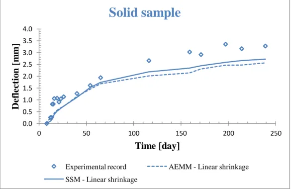
As part of this project an analytical model was derived aimed at predicting the long-term response of concrete members considering different degrees of refinement in the representation of the concrete behaviour. The numerical models were implemented in MATLAB and were used to predict the results measured in previous long-term experiments carried out on post-tensioned composite slabs and on the long-term reinforced concrete slabs tested as part of this project.
The software used to run these analyses is MATLAB. The general idea is that, for a single span beam element, once the curvature is known at three different points, the deflection shape can be interpolated with a 4th order parabola (for detailed calculation refer to paragraph 3.4), while to estimate the curvature of a prismatic element at a given cross section, a cross sectional analysis can be performed. Finally, once the models provide the required deflections, they can be compared with the experimental values.
3.2
Theoretical methodology
3.2.1 Cross Sectional Analysis (CSA)
A cross-sectional analysis (CSA) is a useful tool for the determination of stress and strain distributions at particular locations along a member. The complexity of the analysis and accuracy of the results depend on the assumptions of the formulation and the constitutive models adopted for the materials forming the cross-section.
The CSA is based on the classical Euler-Bernoulli beam assumptions in which plane sections remain plane and perpendicular to the beam axis before and after deformations.
The cross-sectional analysis is formulated with the strain value at the level of the reference axis r and the curvature as the unknowns of the problems. These are calculated enforcing horizontal and rotational equilibrium at the cross-section as follows:
ext A N dA (3.1) and23 ,
x ext A
M
ydA (3.2)where A represents the cross section, depicts the internal stress, N and ext ,
x ext
M are the external axial force and bending moment calculated with respect to the x-axis, respectively.
The calculation of the internal stress is based on the constitutive models specified for the different materials forming the cross-section. These are linear-elastic for the steel reinforcement and profiled sheeting, while for the concrete account for its time-dependent behaviour. Compatibility is enforced calculating the strain for the different material forming the cross-section with the following expression:
y r y (3.3)
where y represents the vertical axis of the cross section.
When adopting the proposed method of analysis one analysis needs to be carried out to evaluate the instantaneous deformations, expressed in terms of the strain at the level of the reference axis and the curvature, while the number of simulations to be performed with time depends on the time-dependent representation adopted for the concrete.
3.2.2 Time-dependent behaviour of concrete
As already described in Chapter 3, creep and shrinkage take place in the concrete over time and different expressions can be adopted for their representation.
The total deformation at time t of a concrete specimen loaded at time 0 can be decomposed in instantaneous, creep and shrinkage components
t, 0
e
0 cr
t, 0
sh
t, 0
(3.4)
The instantaneous and the creep components, e
0 and cr
t,0
, are stressdependent, while the shrinkage component sh
t,0
is not.3.2.2.1 Constant and non uniform shrinkage deformations
The shrinkage deformation can be calculated using some analytical models, but, usually, these kinds of models lead to an excessive simplification of the problem. For this reason, during experimental tests, the shrinkage data is taken
24
directly from the samples, because it represents better the real condition of the main test. But in design, usually, this is not possible and thus the shrinkage is calculated through the formulation provided by the codes. More in detail, in this experiment, shrinkage data is taken from some cylinders and prisms poured the same day of the main test and with the same concrete mix. In addition, these cylindrical and prismatic samples are taken in the same environment of the main specimen and thus also the boundary conditions are exactly the same for both of them. Obviously, this precision cannot be reached using a certain analytical model provided by codes or other experimental tests. Moreover, as obtained from other experimental data collected in the laboratory, shrinkage can occur with different velocities in different parts of the concrete sample, depending on the boundary conditions. For this reason the model should allow for a non-uniform profile input in the cross section of the analysed member. Consequently the shrinkage expression used in this model depends also from the position y in the vertical axis of the cross section, and thus it can be written as
, 0,
shsh t y (3.5)
More in detail, to take into consideration a different shrinkage throughout the depth of the cross section, the general shrinkage deformation is defined as
,
sh r sh shy
(3.6)
where r sh, and sh are respectively the shrinkage strain at the depth position
0
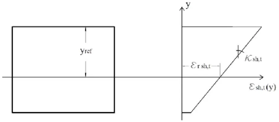
y and the curvature of the shrinkage profile. An illustration of the general shape of a shrinkage strain profile throughout the depth of a cross section is reported in Figure 3.1.
25 At present there are no expressions for the determination of the value for r sh, and sh, and their calculation is based on the limited experimental measurements carried out at the University of Sydney (20). In the laboratory environment readings of free shrinkage were taken on the outside faces and within the thickness of unreinforced concrete samples. Considering the linear distribution measured for the total deformations, the outside face measurements have been used to calculate r sh, and sh as follows:
, ,
, , sh btm sh top ref r sh sh top y D (3.7) , , sh btm sh top sh D (3.8)where sh btm, and sh top, represent the shrinkage at the bottom and the top surfaces of the samples.
3.2.2.2 Principle of superposition - the Step-by-Step Method (SSM) The SSM is based on the principle of superposition. As represented in Figure 3.2, the time period of sustained stress is subdivided into k intervals: at 0 corresponds the first loading after the pour and at k corresponds the end of the time period.
Figure 3.2 – Time discretisation
The general idea is the concrete stress varies between time steps at an increment c
j . Analytically, the constitutive relation for the concrete at any j time step becomes:
1 , , , , , , 0 j c j c j j sh j e j i c i i E F
(3.9)where Ec j, is the instantaneous elastic modulus of concrete and Fe j i, , is the stress modification factor; these terms are defined as
26 , , 1 c j j j E J (3.10) , 1 , , , , j i j i e j i j j J J F J (3.11)
3.2.2.3 Age-adjusted Effective Modulus Method (AEMM)
The AEMM was developed by Trost (21) and its formulation can be expressed as:
, 0
0 ,0c t E te t sh t c Fe (3.12)
where the age-adjusted effective modulus E te
,0
and the coefficient Fe,0 are given by the expressions
0
0 0 0 , 1 , , c e E E t t t (3.13)
0
,0 0 0 0 , 1 , 1 , , e t F t t t (3.14)The function
t, 0
is defined as the ageing coefficient and, as suggested by Gilbert and Ranzi (15), for concrete loaded at early ages
0 20days
it can be approximated to 0.65 while a value of 0.75 is suggested for concrete loaded at later ages
0 28days
.3.3
Detailed expressions of the numerical formulation for a
cracked section
The cross analysis used and developed in this thesis follows the procedure presented in Gilbert and Ranzi’s book Time-dependent behaviour of concrete structures (15). In this thesis, only the main analytical expressions regarding steel and tendon will be showed in the following pages, but take into consideration that the MATLAB scripts are developed including a top and a bottom reinforcement layer, a tendon layer and a deck layer. Thus, the last ones are more complete and useful for a more complex situation. The cross section shape is rectangular. An example of the generic cross section discussed in this numerical formulation is reported in Figure 3.3; but remember that the slabs under examination have a single layer of ordinary steel reinforcement and no
27 prestressed reinforcement layer.
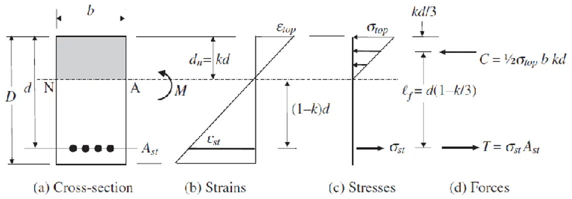
Figure 3.3 – General cross section
The section is crossed by a couple of Cartesian axis located at a distance yref
from the top concrete fibre. There is a bottom ordinary steel reinforcing layer of area A at a distance s y from the reference axis and a post-tensioned strand s layer at a distance yp. Based on the Bernoulli’s hypothesis, the deformation
should be a linear function of the vertical axis y. Therefore the general expression of the total deformation can be written as
y y r (3.15)
where and r are respectively the curvature and the strain at the reference axis level, both of them dependent on time. They are the main unknowns to solve in order to calculate the following stresses in all the structural elements.
The analysis can be divided in two main parts: instantaneous analysis and long-term analysis. In this specific thesis the analysis to carry out is that for a cracked cross section. This case is slightly more complicated than the uncracked cross section case, because the position of the neutral axis moves towards the compressive part of the section every time that part of the section itself cracks in the tensile part.
3.3.1 Age-adjusted Effective Modulus Method
3.3.1.1 Short-term analysis
Assuming an axial force Ne,0 and a bending moment Me,0 about the x-axis sufficiently high to cause a tension stress able to produce the cracking of the bottom fibres and compression in the top ones, the strain at any y depth below the reference x-axis at time 0 is given by:
0 r,0 y 0
28
Once the curvature 0 and the strain at the reference axis level r,0 are found, through the following constitutive relations it is possible to evaluate the stresses in the concrete, in the steel and in the tendon:
,0 ,0 0 ,0 ,0 0 ,0 ,0 ,0 for 0 for c c c r n c n E E y y y y y (3.17)
,0 0 ,0 0 s Es Es r ys (3.18)
,0 0 , ,0 0 , p Ep p init Ep r yp p init (3.19)where Ec,0, E and s Ep are respectively the concrete Young modulus, the steel and the tendon elastic modulus at the time in which the load is applied (i.e.
0
t ), while p init, is the strain in the prestressed steel immediately before the transfer of prestress to the concrete, expressed as
, , p init p init p p P A E (3.20)
The first step in order to find the unknown 0 and r,0 is enforcing equilibrium between the internal and the external axial forces:
,0 ,0 ,0 ,0 e i e i N N M M (3.21)
The internal axial force can be expressed as
,0 ,0 ,0 ,0
i c s p
N N N N (3.22)
where Nc,0, Ns,0 and Np,0 represent the axial forces resisted by the concrete, the ordinary steel and the prestressed steel and they can be calculated as
,0 ,0 ,0 ,0 0 c c c c c r A A N
dA
E y dA (3.23)
,0 ,0 0 ,0 0 , ,0 , 0 s s s s s r s s s r s s s A s r B s N A A E y A E y A E R R (3.24)
,0 ,0 0 , ,0 0 , , ,0 , 0 , p p p p p r p p init p p r p p p p p p init A p r B p p p p init N A A E y A E y A E A E R R A E (3.25)29 Substituting equations (3.23), (3.24) and (3.25) in equation (3.22) and rearranging the expression, it becomes
,0 ,0 ,0 0 , , ,0 , , 0 , c i c r A s A p r B s B p p p p init A N
E y dA R R R R A E (3.26)Thus, using the axial equilibrium condition (Equation (3.21)) and rearranging it, it becomes
,0 , ,0 ,0 0 , , ,0 , , 0 c e p p p init c r A s A p r B s B p A N A E
E y dA R R R R (3.27)Following the exact same procedure, the expression below based on the moment equilibrium can be derived
,0 , ,0 ,0 0 , , ,0 , , 0 c e p p p p init c r B s B p r I s I p A M y A E
E y ydA R R R R (3.28)At this point, two possible solutions are available according to the initial load condition. In the case of a pure bending load Ne,0 Ni,0 0 and no prestress, expression (3.27) becomes a quadratic equation that can be solved to obtain the location of the neutral axis yn,0. Otherwise, in the case of external axial load different from zero or in presence of prestress, the solution can be found dividing equation (3.28) by equation (3.27); in this way, after some analytical passages and recognising that, at the axis of zero strain, y yn,0 r,0 0, the expression becomes:
,0 ,0 ,0 ,0 , , ,0 , , ,0 , ,0 , ,0 ,0 , , ,0 , , n ref n ref y y c n B s B p n I s I p y d e p p p p init y y e p p p init c n A s A p n B s B p y d E y y ydA R R y R R M y A E N A E E y y dA R R y R R
(3.29)Finally equation (3.29) can be solved with a trial and error search and the value yn,0 can be found. Once the portion of uncracked concrete section is known, the properties of the compressive concrete (A , c B and c I ) can be c
30
calculated with respect to the reference axis. Now it is possible to write once again the expressions for Ni,0 and Mi,0 as:
,0 ,0 ,0 ,0 0 , i A r B p p p init N R R A E (3.30) ,0 ,0 ,0 ,0 0 , i B r I p p p p init M R R y A E (3.31)
where RA,0, RB,0 and RI,0 are the axial rigidity and the stiffness respectively related to the first and second moment of area of the cracked section about the reference axis calculated at time 0 and given by:
,0 ,0 ,0 , , A c c s s p p c c A s A p R A E A E A E A E R R (3.32) ,0 ,0 ,0 , , B c c s s s p p p c c B s B p R B E y A E y A E B E R R (3.33) 2 2 ,0 ,0 ,0 , , I c c s s s p p p c c I s I p R I E y A E y A E I E R R (3.34)
Substituting the expression for Ni,0 and Mi,0 (equations (3.30) and (3.31)) into equations (3.21) and (3.22) produces the system of equilibrium equations that may be written in compact form as
,0 0 0 , e p init r D f (3.35) and solved as
1 0 D0 re,0 fp init, F r0 e,0 fp init, (3.36) The quantities used in the previous expression are defined as,0 ,0 ,0 e e e N r M (3.37) ,0 ,0 0 ,0 ,0 A B B I R R D R R (3.38) ,0 0 0 r (3.39) , , , p p p init p init p p p p init A E f y A E (3.40) ,0 ,0 0 2 ,0 ,0 ,0 ,0 ,0 1 I B B A A I B R R F R R R R R (3.41)
31 can be calculated through equations (3.17), (3.18) and (3.19).
3.3.1.2 Long-term analysis
Before starting developing the analytical calculation of this part, it is important to underline the strong assumption at the base of AEMM necessary for a cracked section. It is assumed that the size of the uncracked concrete compressive zone remains constant in time, even if, for the presence of the sustained load, creep induces a movement of the neutral axis position. However, since the assumption simplifies considerably the calculation and since the corresponding error is little it will be used in the AEMM analysis.
In the case of axial force and uniaxial bending, the analytical calculations used for a cracked section are very similar to those used for an uncracked section. For long-term analysis, the steps to follow in order to find the unknowns are almost the same of the instantaneous analysis, except for some details; first of all, the Young modulus of the concrete should be substituted with the effective modulus and then the terms related to shrinkage, creep and relaxation of strands should be added. These last three terms are responsible for the time dependency. Analytically, each of them will give an additional contribution to equation (3.35) at the end of all the analytical passages.
Assuming a linear-elastic behaviour (as for the short-term analysis) of the steel reinforcement and the prestressing tendons (if any) and a constitutive relationship similar to equation (3.12) for concrete, the new constitutive relationships become
, , , ,0 ,0 ,0 , ,0 for 0 for c k e k k sh k e c n c k n E F y y y y (3.42) , s k Es k (3.43)
, , , , p k Ep k p init p rel k (3.44)where Ee k, and Fe,0 are as defined previously (equations (3.13) and (3.14)) and the tensile creep strain p rel k, , , also referred as relaxation strain, is calculated as the product between a design relaxation coefficient R (clause 3.3.4 of the Australian Standard (2)) and the initial strain in the prestressing steel before transfer:
, , ,
p rel k p initR
32
Once again, as in the instantaneous analysis, to solve the problem it is necessary to impose equilibrium between internal and external forces at time k:
, , , , e k i k e k i k N N M M (3.46)
As before, the axial force Ni k, is
, , , ,
i k c k s k p k
N N N N (3.47)
and the three components are
, , , , , ,0 ,0 , , , , , ,0 ,0 , , , , , ,0 ,0 c c c k c k e k r k k sh k e c A A c e k r k c e k k c e k sh k e c A c r k B c k A c sh k e c N dA E y F dA A E B E A E F N R R R F N
(3.48) , , , , , s k s s r k s s s k A s r k B s k N A E y A E R R (3.49)
,0 , , , , , , , , , , , p p p r k p p p k p p p init p rel k A p r k B p k A p p init p rel k N A E y A E A E R R R (3.50)Defining the axial rigidity RA k, and the stiffness related to the first moment of area RB k, at time k as , , , , A k A c A s A p R R R R (3.51) , , , , B k B c B s B p R R R R (3.52)
equation (3.47), after some substitutions can be rewritten as
, , , , , , ,0 ,0 , , , ,
i k A k r k B k k A c sh k e c A p p init p rel k
N R R R F N R (3.53)
Using the same procedure, the internal moment Mi k, resisted by the cross section at time k can be expressed as:
, , , , , , ,0 ,0 , , , ,
i k B k r k I k k B c sh k e c B p p init p rel k
M R R R F M R (3.54)
with the stiffness related to the second moment of area RI k, at time k equal
33
, , , ,
I k I c I s I p
R R R R (3.55)
Note that the quantities Nc,0 and Mc,0 present in equations (3.53) and (3.54) are known from the instantaneous analysis.
Substituting equations (3.53) and (3.54) into equation (3.46), the following compact form can be written
, , , , , , e k k k cr k sh k p init p rel k r D f f f f (3.56) where , , , e k e k e k N r M (3.57) , r k k k (3.58) , , , , A k B k k B k I k R R D R R (3.59)
The creep effect produced by the stress c,0 resisted by the concrete at time 0
is represented by the vector
,0 ,0 0 , ,0 ,0 ,0 ,0 ,0 0 c c r c cr k e e c c c r c N A B f F F E M B I (3.60)
while the shrinkage strain vector fsh k, can be calculated as
, , , , , , c c c c sh k e k sh k e k r sh k k c c c c A B A B f E E B I B I (3.61)
The vectors fp init, and fp rel k, , account respectively for the initial prestress and for the resultant actions caused by the loss of prestress in the tendon due to relaxation. They are given by:
, , , p p p init p init p p p p init A E f y A E (3.62) and , , , p rel k p init f f R (3.63) Solving equation (3.56):