Bayesian semiparametric approaches to mixed-effects models with an application in reliability analysis

(1)

Politecnico di Milano

Facolt`a di Ingegneria dei Sistemi

Corso di Laurea in Ingegneria Matematica

Tesi di Laurea Specialistica

Bayesian semiparametric approaches to

mixed-effects models

with an application in reliability analysis

Candidato: Jacopo Soriano Matricola 735664

Relatore: Prof.ssa Alessandra Guglielmi Correlatore: Dott. Raffaele Argiento

(2)

“Prediction is very difficult, especially about the future.”

(3)

Ringraziamenti

Molte persone hanno permesso, in modo pi`u o meno diretto, che io arrivassi a realizzare questa tesi e questo `e il luogo per esprimere loro tutta la mia gratitudine.

Un primo ringraziamento va alla professoressa Alessandra Guglielmi per avermi guidato con entusiasmo e attenzione durante tutto il lavoro della tesi, e per aver dimostrato grande fiducia nelle mie capacit`a e nella mia persona. Ringrazio molto anche il dottor Raffaele Argiento per la totale disponibilit`a e per il buon umore con cui ha risposto a tutte le mie domande.

Un grazie alla mia famiglia che `e sempre stata un punto di riferimento: mi ha sostenuto nelle situazioni difficili e ha gioito con me in quelle felici. Un grazie a mia nonna Dina che mi ha trasmesso la passione per la matematica sin dalle tabelline.

Un grazie a tutti gli amici del Liceo, del Politecnico e di Centrale con i quali ho potuto confrontarmi e crescere tra e fuori dai banchi.

(4)

List of Figures

3.1 Photos of the NASA pressure vessels from the 2009 Composite Pressure Vessel and Structure Summit [5]. . . 26 4.1 Marginal error distribution density functions for different hyperparameters

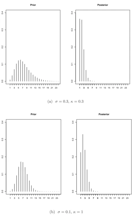
of the gamma prior for the shape parameter θ. (a) Marginal error of Leon et al.’s parametric model, and (b) marginal error used in our semiparametric models. . . 37 4.2 Prior and posterior number of mixture components for the model with

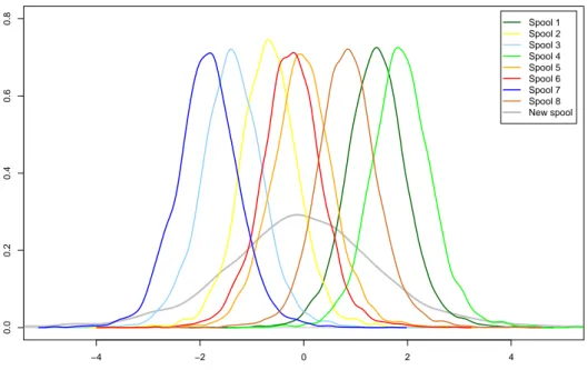
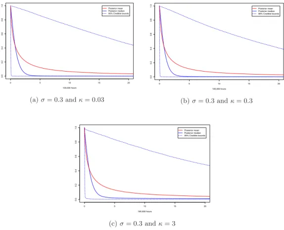
non-parametric error . . . 42 4.3 Posterior kernel density estimation of the random effects for the model with

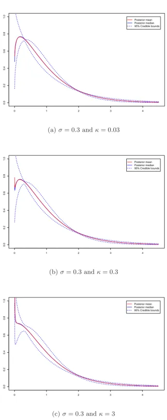
nonparametric error (σ = 0.3 and κ = 0.3) . . . . 44 4.4 Posterior marginal density distribution functions of the error in the model

with nonparametric error . . . 45 4.5 Survival functions for a new random spool at 22.5MPa for the model with

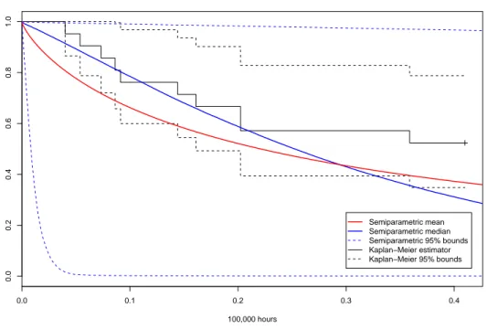
nonparametric error . . . 46 4.6 Predicted survival functions for a new random spool at 23.4MPa for the

model with nonparametric error (σ = 0.3, κ = 0.3), and for Kaplan-Meier estimator . . . 47 4.7 Bayesian residuals for the uncensored failure times under the model with

nonparametric error (σ = 0.3, κ = 0.3). . . . 49 4.8 Markov chain sample of β0, β1 and α1 . . . 50

4.9 Scatterplot of the log-survival times against the log-stress for the two semi-parametric models. . . 53 4.10 Posterior kernel density estimation of the random effects for the model with

nonparametric random effects (σ = 0.3 and κ = 1.2) . . . . 57 4.11 (a) Posterior kernel density estimation of the shape parameter θ and (b)

posterior marginal density distribution function of the error for the model with nonparametric error, where σ = 0.3 and κ = 1.2. . . . 57 4.12 Predicted survival functions for a new random spool for the model with

(7)

4.13 Bayesian residuals against the fitted log failure times . . . 59 4.14 Bayesian residuals against the quantiles of the Gumbel standard at the four

stress levels . . . 60 4.15 Markov chain sample of β1 and α1 . . . 61

4.16 Density distribution function of the marginal error V for different choices of the hyperparameters a0 and b0 . . . 62

(8)

List of Tables

3.1 Mechanical properties of a single fiber and a single yarn of Kevlar . . . 26 4.1 Interval estimates of the quantiles of the predictive distributions for the

parametric model . . . 38 4.2 Interval estimates of the quantiles of the predictive distributions for the

model with nonparametric error for different hyperparameters of the NGG process prior. . . 40 4.3 Interval estimates of the quantiles of the predictive distributions for the

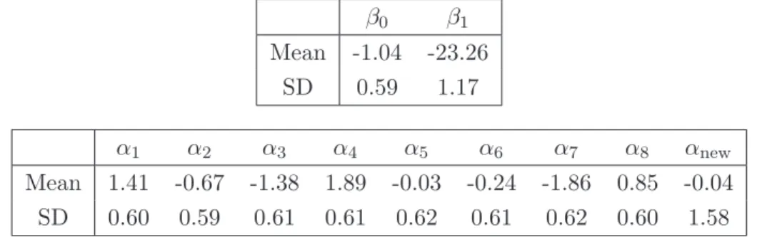
model with nonparametric error (σ = 0.3, κ = 0.3) . . . . 41 4.4 Posterior mean and standard deviation (SD) of the effects for the model

with nonparametric error (σ = 0.3 and κ = 0.3) . . . . 43 4.5 Interval estimates of the quantiles of the predictive distributions for different

number of grid points for the model with nonparametric error (σ = 0.3, κ = 0.1). . . . 51 4.6 Interval estimates of the quantiles of the predictive distributions for the

model with nonparametric random effects (σ = 0.3, κ = 1.2) . . . . 54 4.7 Interval estimates of the quantiles of the predictive distributions for the

model with nonparametric random effects for different hyperparameters of the NGG process prior. . . 55 4.8 Posterior mean and standard deviation (SD) of the effects for the model

with nonparametric random effects (σ = 0.3 and κ = 1.2) . . . . 56 4.9 Interval estimates of the quantiles of the predictive distributions for the

model with gamma error for different hyperparameters of the dispersion parameter θ (a ∼ Gamma(a1 = 1, b1= 1)). . . 63

4.10 Interval estimates of the quantiles of the predictive distributions for the model with gamma error for different hyperparameters of the mass param-eter a (θ ∼ Gamma(a0= 1, b0 = 1)). . . 63

4.11 Interval estimates of the quantiles of the predictive distributions for the model with gamma error (θ ∼ Gamma(a0 = 1, b0 = 1) and a ∼ Gamma(a1 =

(9)

4.12 Posterior mean and standard deviation (SD) of the effects for the model with gamma error (θ ∼ Gamma(a0 = 1, b0= 1) and a ∼ Gamma(a1 = 1, b1 = 1)) 64

C.1 Failure-times of NASA pressure vessels wrapped with Kevlar. Right-censored observations are indicated with an asterisk *. . . 80

(10)

Abstract

Questo lavoro si prefigge un duplice obiettivo: da una parte quello di effettuare uno studio metodologico sui modelli ad effetti casuali in ambito bayesiano non parametrico, dall’altro di utilizzare questi modelli in un problema di affidabilità. Dopo una breve introduzione all’approccio bayesiano non parametrico, segue la costruzione del processo gamma gen-eralizzato normalizzato (NGG) a partire da misure di probabilità aleatorie a incrementi indipendenti, e una descrizione delle principali proprietà. Tale processo sarà utilizzato come ingrediente nei modelli presentati in seguito. I test di rottura accelerata (ALT) sono test di affidabilità in cui si accelera il processo di rottura di un pezzo meccanico con l’obiettivo di estrapolare quale sarà la vita del componente a condizioni di stress normali. I dati relativi a un ALT possono essere analizzati con un modello accelerated failure time (AFT) in cui si cerca di comprendere il legame tra il logaritmo del tempo di rottura e alcune variabili esplicative. In questo lavoro analizziamo un ALT effettuato dalla NASA su alcuni recipienti in pressione dello Space Shuttle. I recipienti sono rivestiti con Kevlar proviente da diversi rocchetti e trattiamo l’effetto del rocchetto come casuale. I tempi di rottura sono rappresentati con due modelli AFT bayesiani semiparametrici, con l’obiettivo di fornire intervalli di credibilità per determinati quantili della distribuzione del tempo di vita di un recipiente rivestito con Kevlar proveniente da un nuovo rocchetto. Nel primo modello, l’errore è rappresentato da una mistura di distribuzioni parametriche in cui la misturante è un processo NGG. Nel secondo modello, gli effetti casuali vengono considerati in modo non parametrico, utlizzando una prior di tipo NGG. Per entrambi i modelli ab-biamo calcolato analiticamente le espressioni delle full-conditional necessarie per poter costruire un algoritmo MCMC che permetta di campionare dalla distribuzione a posteri-ori; quindi abbiamo implementato gli algoritmi in C ed eseguito simulazioni numeriche. In particolare, nel primo modello ad ogni iterazione dell’algoritmo simuliamo una traiettoria dal processo NGG, mentre nel secondo usiamo un algoritmo di tipo Polya-urn.

(11)

Abstract

In this work we provide a methodological study about Bayesian nonparametric random-effects models, and an application of these models in reliability. After a brief introduction to the nonparametric Bayesian approach, the construction of the normalized generalized gamma process (NGG) by normalization of a completely random measure is provided. This process is an ingredient of the models we will introduce later. Accelerated life testing (ALT) involves acceleration of failure times with the purpose of predicting the life-time of the product at normal use conditions. Data from an ALT can be analyzed by a so-called Accelerated Failure Time (AFT) model, where the dependence between the logarithm of the failure time is related to some explanatory variables. We analyze an AFT made by NASA on some pressure vessels, which are critical components of the Space Shuttle, via two semi-parametric Bayesian AFT models. The pressure vessels are wrapped with Kevlar from different spools and we treated the spool effect as random. In particular, we provide credibility intervals of some given quantiles of the failure-time distribution for a pressure vessel wrapped with fiber from a new random spool. In the first model the error is represented by a mixture of parametric distribution with a NGG mixing measure, while in the second one the random effects have a NGG process prior. For both models, we derived the analytical expressions of the full-conditional distributions needed to make a MCMC algorithm to sample from the posterior distribution; then we coded the algorithms in C and we made numerical simulations. In particular, at each iteration of the first models algorithm, we sample a trajectory of the NGG process; while in the second model, we implemented a Polya-urn scheme algorithm.

(12)

Introduzione

Questo lavoro si prefigge un duplice obiettivo: da una parte quello di effettuare uno studio metodologico sui modelli ad effetti casuali in ambito bayesiano non parametrico, dall’altro di utilizzare questi modelli in un problema di ingegneria dell’affidibilit`a.

I modelli ad effetti casuali sono modelli che separano la variabilità tra diverse unità statistiche (gruppi) dalla variabilità all’interno di ogni singola unità. Questi modelli ven-gono anche chiamati modelli gerarchici in quanto permettono appunto di definire due o più livelli di variabilità. Vengono spesso applicati in ambito clinico, ad esempio, dove vengono ripetute diverse osservazioni (misurazioni) per ogni paziente con l’obiettivo di cogliere sia eventuali differenze tra i pazienti sia variazioni a livello del singolo soggetto; in questo caso il fattore di raggruppamento è il paziente. Questi modelli vengono utilizzati anche in altri ambiti, tra i quali citiamo l’analisi di affidabilità di cui ci occuperemo più tardi. Un’ampia classe di modelli ad effetti casuali è quella dei modelli lineari generalizzati a effetti misti (GLMM) in cui gli effetti sono sia fissi che casuali, e in cui si assume che le risposte abbi-amo distribuzione appartenente alla famiglia esponenziale. Secondo Gelman [13], diremo che un effetto è fisso se è identico per tutti gruppi, e casuale se varia da gruppo a gruppo. L’approccio bayesiano agli effetti casuali ha diversi vantaggi rispetto a quello frequen-tista. Prima di tutto l’inferenza frequentista si basa su stime asintotiche, mentre in ambito bayesiano è sempre possibile fare inferenza esatta anche per data-set di piccola dimensione, utilizzando metodi di integrazione numerica Markov Chain Monte Carlo (MCMC). Inoltre, in statistica classica gli effetti casuali tipicamente sono assunti tra loro indipendenti; men-tre in statistica bayesiana vengono assunti scambiabili e questo legame tra gli effetti rende le stime più accurate. In particolare, si ottengono stime ragionevoli anche per quelle unità statistiche, rappresentate dagli effetti casuali, che contengono pochi soggetti. Ricordiamo che l’assunzione di scambiabilità è ragionevole in quanto le unità statistiche possono essere interpretate come un campione senza rimpiazzo dalla popolazione delle unità statistiche.

Spesso non `e ragionevole fare specifiche assunzioni sulla distribuzione degli effetti casu-ali e quindi, in questi casi, l’utilizzo di un modello parametrico porterebbe a stime distorte dei parametri del modello. L’approccio non parametrico rilassa l’ipotesi di appartenenza di una distribuzione ad una classe parametrica, permettendo di superare la dipendenza da

(13)

assunzioni parametriche. Inoltre una prior non parametrica risulta pi`u flessibile e permette un’inferenza pi`u robusta.

Il limite dei modelli bayesiani non parametrici è il grande sforzo computazionale richiesto, anche se la crescente disponibilità delle capacità di calcolo degli ultimi anni ha reso molto popolare l’inferenza bayesiana non parametrica e ha portato ad una grossa produzione di modelli bayesiani non parametrici in letteratura. Nonostante ciò l’onere computazionale è tuttora un problema di primaria importanza e quindi la ricerca di al-goritmi sempre più efficienti resta attuale. Per una presentazione delle più comuni classi di prior non parametriche e dei principali tecniche di inferenza non parametrica si veda Müller e Quintana [29]. Di recente, l’approccio bayesiano non parametrico ha riscontrato successo soprattutto in biostatistica; si veda Dunson [7] per una descrizione esaustiva dei più recenti modelli bayesiani non parametrici utilizzati in questo ambito. In questo la-voro concentriamo la nostra attenzione sulla prior nonparametrica Normalized Generalized Gamma Process (processo NGG). Questo processo, introdotto da Brix [3] nella versione non normalizzata e studiato per la prima volta come prior da Regazzini et al. [35], si costruisce come normalizzazione di una misura completamente aleatoria e comprende il processo di Dirichlet come caso particolare. Cos`ı come il processo di Dirichlet, il pro-cesso NGG seleziona distribuzioni discrete con probabilità uno, e induce una partizione aleatoria sugli interi positivi; in particolare, questo vuol dire che se consideriamo un cam-pione aleatorio di ampiezza n da questo processo, tra le n realizzazioni ci potranno essere dei valori ripetuti e questi valori ripetuti definiscono una partizione degli interi 1, . . . , n. Questa partizione aleatoria è governata da due parametri nel caso dell’NGG, a differenza del processo di Dirichlet in cui il clustering è governato da un solo parametro. Questo ulteriore grado di libertà rende il clustering più ricco e quindi la prior più flessibile.

I test di rottura accelerata (ALT) hanno grande importanza in affidabilità. Si tratta di test in cui si accelera il processo di rottura di un pezzo meccanico con l’obiettivo di estrap-olare quale sarà la vita del componente a condizioni di stress normali. I dati relativi ad un ALT posso essere analizzati con i cosiddetti modelli ”accelerated failure time” (AFT) in cui si cerca di comprendere il legame fra il logaritmo del tempo di rottura (o tempo di vita) e alcune variabili esplicative come ad esempio la pressione o la temperatura; si tratta dunque, in scala logaritmica, di un modello di regressione lineare. Spesso è ragionevole assumere che il tempo di rottura abbia distribuzione Weibull: visto che la distribuzione Weibull non appartiene alla famiglia esponenziale, il corrispondente modello AFT non è un modello lineare generalizzato ma una sua naturale estensione. In questo lavoro analizzer-emo un ALT effettuato dalla NASA su alcuni recipienti in pressione dello Space-Shuttle. Il data-set consiste di 108 tempi di rottura di questi particolari recipienti in pressione ricoperti in fibra di Kevlar, soggetti a 4 livelli di stress, e con fibra proveniente da 8 diversi rocchetti. Il problema dell’affidabilità di questi recipienti è ancora di attualità, infatti nel

(14)

2009 la NASA ha organizzato il Composite Pressure Vessel and Structure Summit [5] per discutere i progressi in questo ambito.

In questo lavoro i tempi di rottura vengono modellati attraverso un modello AFT bayesiano semiparametrico, con l’obiettivo di fornire intervalli di credibilità per determi-nati quantili della distribuzione del tempo di vita di un nuovo recipiente ricoperto con fibra di Kevlar proveniente da un nuovo rocchetto. Dal momento che abbiamo diverse osser-vazioni per ogni rocchetto, risulta naturale considerare l’effetto del rocchetto come casuale; mentre trattiamo l’effetto della pressione come effetto fisso. Questo data-set è stato studi-ato da diversi autori con approcci frequentisti, in cui sia rocchetto che pressione venivano trattati come effetti fissi; più recentemente Leon et al. [24] invece hanno proposto un mod-ello AFT bayesiano parametrico ad effetti misti. Riteniamo che le stime ottenute siano insoddisfacenti e che alcune scelte degli iperparametri delle prior di quest’ultimo modello siano poco ragionevoli. In particolare, riteniamo che gli intervalli di credibilità per de-terminati quantili della distribuzione del tempo di vita siano troppo larghi, e che alcune prior siano eccessivamente informative. Quindi abbiamo deciso di formulare dei modelli più flessibili per ottenere delle stime dei quantili di interesse più robuste e più accurate. Due sono i modelli bayesiani semiparametrici considerati. Nel primo l’errore (di regres-sione) rappresentato da una mistura di distribuzioni parametriche in cui la misturante un processo NGG; la distribuzione degli effetti casuali parametrica, come in Leon et al. [24]. Nel secondo modello l’errore è stato trattato parametricamente come in Leon et al. [24], mentre gli effetti casuali sono stati considerati in modo non parametrico, utilizzando sempre una prior di tipo NGG. Infine abbiamo validato i risultati ottenuti utilizzando la funzione DPglmm nel pacchetto DPpackage del software R. Si tratta di un pacchetto che permette di fare inferenza bayesiana su modelli semi-parametrici; in particolare con la funzione DPglmm si può fare inferenza per modelli GLMM in cui gli effetti casuali hanno una distribuzione iniziale di tipo processo di Dirichlet. Abbiamo utilizzato errori di tipo Gamma, dato che la Weibull non appartiene alla famiglia esponenziale e non è contem-plata in questo pacchetto; ma sottolineiamo che abbiamo usato questo package solo per fare un’analisi comparativa.

I modelli che abbiamo qui sviluppato non solo sono nuovi perchè mai applicati a questo specifico data-set, ma risultano originali anche nel contesto più generale di af-fidabilità bayesiana non parametrica. Infatti, a differenza dell’ambito biostatistico, la letteratura bayesiana nonparametrica in affidabilità non è molto estesa. Inoltre nella parte applicativa della tesi, abbiamo autonomamente calcolato analiticamente le espres-sioni delle full-conditional necessarie per poter costruire un algoritmo MCMC che permetta di campionare dalla distribuzione a posteriori; successivamente abbiamo implementato gli algoritmi nel linguaggio C ed eseguito molte simulazioni numeriche. Per quanto riguarda il primo modello, ad ogni iterazione dell’algoritmo simuliamo traiettorie dal processo NGG.

(15)

Gli algoritmi che simulano intere traiettorie di misure di probabilità aleatorie sono stati proposti recentemente in letteratura; sono in generale molto onerosi dal punto di vista computazionale e di difficile implementazione, ma forniscono un’informazione decisamente più ricca sul modello. Nello specifico per simulare le traiettorie del processo NGG è stato necessario invertire la funzione gamma troncata, che è nota per le sue instabilità nu-meriche; per fare ciò in maniera efficace abbiamo utilizzato la libreria di C chiamata pari. Nel secondo modello abbiamo utilizzato un algoritmo di tipo Polya-Urn che marginalizza rispetto al processo NGG, e che quindi risulta computazionalmente meno pesante.

Nel Capitolo 1, dopo una breve introduzione all’approccio bayesiano non parametrico, vengono presentate le principali proprietà del processo di Dirichlet. Segue la costruzione del processo NGG a partire da misure di probabilità aleatorie a incrementi indipendenti. In ultimo vengono descritte le proprietà del processo NGG.

Nel Capitolo 2 vengono introdotti i GLMM. Questa classe di modelli nasce dall’unione dei modelli lineari ad effetti misti in cui la risposta ha distribuzione gaussiana e gli effetti sono sia fissi che casuali, e i modelli lineari generalizzati che hanno risposta appartenente alla classe della famiglia esponenziale ed effetti fissi. Ci concentriamo in particolare sui modelli lineari generalizzati a effetti misti in ambito bayesiano: partiamo dal caso para-metrico proposto da Zeger e Karim [38]; per poi giungere a quello semi-parapara-metrico di Kleinmann e Ibrahim [23], in cui gli effetti casuali hanno prior nonparametrica di tipo processo di Dirichlet.

Nel Capitolo 3 viene introdotta qualche nozione relativa all’analisi di sopravvivenza (ricordiamo che in ambito ingegneristico questa prende il nome di analisi di affidabilit`a), e poi viene presentato il data-set relativo ai recipienti in pressione dello Space-Shuttle. In ultimo vengono introdotti i modelli AFT bayesiani menzionati in questa Introduzione: il modello parametrico di Leon et al. [24], il modello con errori nonparametrici, il modello con effetti casuali non parametrici e quello con errori gamma del pacchetto DPpackage.

Nel Capitolo 4 presentiamo e confrontiamo i risultati ottenuti dai vari modelli. Per ogni modello discutiamo la scelta degli iperparametri della prior, forniamo gli intervalli di credibilit`a dei quantili di interesse della distribuzione del tempo di vita per un nuovo recipiente in pressione, le stime a posteriori dei parametri del modello e l’analisi dei residui. Le Appendici A e B riportano le espressioni analitiche delle full-conditional rispet-tivamente del modello con errori non parametrici e del modello con effetti casuali non parametrici.

(16)

Introduction

In this work we provide a methodological study about Bayesian nonparametric random-effects models, and an application of these models in reliability.

Random-effects models separate the variability among different statistical units (or groups) from the variability inside each statistical unit. These models are also called hierarchical models since they define two or more levels of variability. For instance, they are often used in clinical trials where several observations (measurements) for each patient are taken to estimate differences among patients and the variability within each patient; in this case the grouping factor is the patient himself. These modeling techniques have application in several fields, reliability analysis among others. A wide class of random-effects models is that of the generalized linear mixed-random-effects models (GLMMs), where the effects are both fixed and random, and the outcome belongs to the exponential family. There are several, and often conflicting, definitions of fixed and random-effects. By Gelman [13], fixed-effects are identical for all groups in a population, while random-effects are allowed to differ from group to group.

The Bayesian approach to random effects have several advantages with respect to the frequentist one. First, frequentist inference is often based on asymptotic assumptions, while in the Bayesian framework it is always possible to make exact inference using Markov Chain Monte Carlo (MCMC) numerical integration methods, for data-set of any dimen-sion. Moreover, in classical statistics the random-effects parameters are generally consid-ered mutually independent; on the other hand in Bayesian statistics they are assumed exchangeable and this dependence among the effects brings to more accurate estimates. In particular, exchangeability enables to borrow strength across random-effects and so we obtain reasonable estimates also for the statistical units with few observations. We recall that the exchangeability assumption is reasonable here, since the statistical units, represented by the random-effects, could be considered as a sample without replacement from the population of statistical units.

Often it is not reasonable to make any parametric assumption about the random-effects’ distribution and so, in these cases, a parametric model could bring to biased esti-mates of the parameters. The nonparametric approach relaxes the parametric hypothesis

(17)

for the random-effects and leads to a more robust inference.

The drawback of the Bayesian nonparametric approach consists in its computational heaviness, but the increasing computational power of the last years has made Bayesian nonparametric inference feasible and more popular in literature. However, the computa-tional efforts required for the inference is still one limitation of Bayesian nonparametrics and hence the research of efficient algorithms is always up-to-date. See M¨uller and Quin-tana [29] for a presentation of the most common classes of nonparametric priors and of the main Bayesian nonparametric inference’s techniques. Recently, Bayesian nonparametrics has become particularly popular in biostatistics; see Dunson [7] for an exhaustive descrip-tion of the latest Bayesian nonparametric models in this field. In this work we focus on the Normalized Generalized Gamma (NGG) process prior. This process was introduced by Brix [3] in its unnormalized version, while Regazzini et al. [35] studied it as a prior for the first time. The NGG process can be constructed by normalization of a completely random measure, and the Dirichlet process is recovered as a particular case. Like the Dirichlet process, the NGG process selects discrete distributions with probability one, and induces a random partition on the positive integers; in particular, this means that, given a sample of size n from this process, among the n observations there could be repeated values, and these repeated values define a partition of {1, . . . , n}. This random partition is ruled by two parameters in the NGG case, while the grouping of the Dirichlet process is ruled by only one parameter. This additional degree of freedom makes the clustering of the NGG process prior more flexible.

The accelerated life tests (ALTs) are very important in reliability. ALT testing involves acceleration of failure times with the purpose of predicting the life-time of the product at normal use conditions. Data from an ALT can be analyzed by a so-called Accelerated Failure Time (AFT) model, where the dependence between the logarithm of the failure time is related to some explanatory variables like pressure and temperature, among others. Notice that in log-scale this is a regression model. A common choice in AFT models is the Weibull distribution for the life-time, because it has a natural interpretation of the shape and scale parameters. The AFT model is not exactly a GLMM, since the Weibull distribution does not belong to the exponential family, but it can be considered a straightforward generalization. Here, we will analyze an AFT made by NASA on some pressure vessels, which are critical components of the Space-Shuttle. The data-set consists of 108 lifetimes of pressure vessels wrapped with Kevlar yarn. The fiber of Kevlar comes from 8 different spools and 4 levels of pressure stress are used. The reliability of the pressure vessels is still relevant: in 2009 NASA organized the Composite Pressure Vessel

and Structure Summit [5] to discuss the state of the art on this subjet.

In this work, we model the failure times via semi-parametric Bayesian AFT models, and provide posterior estimates of the regression parameters and credibility intervals of

(18)

some given quantiles of the failure-time distribution for pressure vessel wrapped with fiber from a new random spool. We consider the spool effect as random, since several observa-tions for each spool are provided, while the pressure stress level is treated as a fixed effect. Several authors studied this data-set with a frequentist approach, where both spool and pressure are considered as fixed effects; more recently Leon et al. [24] fitted a Bayesian parametric AFT model with mixed-effects. Their estimates are not completely reliable and some of their prior assumptions are questionable. According to our opinion, some of their interval estimates of given quantiles of the failure-time distribution are too large, the hyperparameters of the prior are too much informative, and their posterior estimates are affected by a large Monte Carlo error. Hence, we assumed more flexible models with the purpose of getting more accurate and more robust estimates. We studied two different Bayesian semiparametric models. In the first model, the regression error is represented by a mixture of parametric distribution with a NGG mixing measure, while the distribution of the random-effects is parametric as in Leon et al. [24]. In the second model, the error is treated parametrically as in Leon et al. [24], while we consider nonparametric random-effects, using a NGG process prior. Finally, we validated our results using the function

DPglmm of the package DPpackage in the statistical software R. This package offers

several functions to fit Bayesian nonparametric and semiparametric models; in particular the function DPglmm fits GLMMs, where the random-effects have Dirichlet process prior distribution. The outcome is assumed here Gamma-distributed, since the Weibull distri-bution does not belong to the exponential family and it is not available in this package. We underline that we used DPpackage only for comparative purposes only.

Not only these models are new for this given data-set, but also in the more general framework of reliability under a Bayesian approach. In fact, despite biostatistics, relia-bility nonparametric Bayesian literature is not particularly wide. Moreover, we derived the analytical expressions of the full-conditional distributions needed to make a MCMC algorithm to sample from the posterior distribution; then we coded the algorithms in the programming language C and we made several numerical simulations. At each iteration of the first model’s algorithm, we sample a trajectory of the NGG process. The algorithms that simulate complete trajectories of random probability measures are quite recent in literature; they are particularly time consuming and hard to implement, but they provide much information on the model. In particular, to sample a trajectory of the NGG process, we must invert the truncated gamma function, which is well-know for its numerical insta-bility(we used a C library called pari). In the second model, we implemented a Polya-urn

scheme algorithm, which integrates out the NGG process, and so it is computationally

less heavy.

In Chapter 1, after a brief introduction to nonparametric Bayesian approach, we present the main properties of the Dirichlet process. Then a construction of the NGG

(19)

process by normalization of a completely random measure is provided. Finally, we intro-duce the main properties of the NGG process.

In Chapter 2 we present the GLMM. This class of models can be seen as the gen-eralization of mixed-effects linear models and generalized linear models. We will focus on the Bayesian approach to GLMM: first, we introduce the parametric model of Zeger and Karim [38]; then the semi-parametric one of Kleinmann and Ibrahim [23], where the random effects have Dirichlet process prior.

In Chapter 3 we provide basic notions of survival analysis (or reliability analysis in engineering), and then we introduce the data-set of the NASA pressure vessels. Finally, we present the Bayesian AFT models mentioned before: Leon et al.[24]’s parametric model, the model with nonparametric error, the model with nonparametric random-effects, and the model with Gamma-distributed error of DPpackage.

In Chapter 4 we present and compare the results of the different models. For each of them, we discuss the prior hyperparameter’s choice, and we provide the interval estimates of given quantiles of the failure time distribution for a new pressure vessel wrapped with fiber from a new random spool, the posterior estimates of the parameters and the analysis of the residuals.

In Appendix A and B we provide the analytic expressions of the full-conditionals of the model with nonparametric error and those of the model with nonparametric random-effects, respectively.

(20)

Chapter 1

Bayesian Nonparametrics

1.1 Exchangeability assumption

Classical statistics is based on a framework where observations X₁, X₂. . . are assumed

independent and identical distributed (i.i.d.) from a unknown probability distribution P . We say that we are considering a parametric framework when P belongs to a parametric family, otherwise we are considering a nonparametric framework when P lies in the space of probability distributions P(R).

It is possible to distinguish the two cases also in the Bayesian setting. In the parametric case we have a prior Π on a finite dimensional space Θ and, given θ, the observations are assumed i.i.d. from P_θ. In the nonparametric case, we have a prior Π on the space P(R) of all probability distributions on (R, B(R)) and, given P , the observations are assumed i.i.d. from P .

Under the assumption of exchangeability, de Finetti’s Representation Theorem gives a validation of the Bayesian setting.

Let consider an infinite sequence of observations (Xn)n≥1 defined on some probability space (Ω, F, P), with each X_i taking values on R endowed with the Borel σ-algebra B(R). This last hypothesis can be relaxed and we could consider observations which take values in a complete metric and separable space X. In this work it is enough to consider X = R. Definition 1. A sequence (Xn)n≥1 is exchangeable when, for any finite permutation π of (1, 2, . . . , n), the random vectors (X₁, . . . , X_n) and (X_π(1), . . . , X_π(n)) have the same

probability distribution.

There are several types of dependence among a sequence of observations (Xn)n≥1. Under the exchangeability assumption, the information that the observations Xis provide is independent of the order in which they are collected. For instance, if we sample without

(21)

replacement from an urn with infinite marbles of different colors, the sequence of colors that we obtain is exchangeable.

A random element defined on (Ω, F, P), with values in P(R), is called random

proba-bility measure (r.p.m.).

With a view to our utilization of r.p.m.s in statistics, the two main desirable properties for the class of r.p.m. are a large support, and a posterior distribution that is analytically tractable. A prior with a large support is an obvious requirement, and a tractable pos-terior reduces the computational complexity. In fact computational heaviness is still one limitation of Bayesian nonparametrics.

The most popular r.p.m.s in literature are Dirichlet Processes, Polya Trees and Bern-stein Polynomials. A recent review of the main r.p.m. classes appears in M¨uller and Quintana [29].

Now we give formal definitions of the Borel σ-algebra on P(R) introducing the topol-ogy of weak convergence. The space P(R) is equipped with the topoltopol-ogy of the weak convergence which makes it a complete and separable metric space. We will write that

Pn−→ P (Pw n converges weakly to P ), if Z R f dPn→ Z R f dP, as n → +∞

for all bounded continuous function f on R. For any P0 a neighborhood base consists of

sets of the form

∩k_i=1{P : |

Z

f_idP₀−

Z

f_idP | < ²}

where fi, i = 1, . . . , k are bounded continuous function on R, k ≥ 1 and ε > 0.

The Borel σ-algebra on P(R) is the smallest σ-algebra generated by the open sets in the weak topology.

Theorem 1 (de Finetti). The sequence (Xn)n≥1 is exchangeable if, and only if, there exists a unique probability measure q on P(R) such that, for any n ≥ 1 and any Borel sets B1, B2, . . . , Bn, P(X1 ∈ B1, X2∈ B2, . . . , Xn∈ Bn) = Z P(R) n Y i=1 p(Bi)q(dp). Equivalently, X1, . . . , Xn|P iid∼ P P ∼ q(·).

(22)

In the parametric case q is concentrated on a parametric family

X1, . . . , Xn|θiid∼ fθ(·) θ ∼ π(·),

where Xi|θ and θ are absolutely continuous (with respect to the Lebesgue measure) or discrete probability distributions, for i = 1, . . . , n. f_θ(·) and π(·) are the probability density functions of Xi|θ and θ respectively.

By Bayes’ Theorem, the posterior probability distribution of θ, i.e. the conditional probability distribution of θ given X₁, . . . , X_n, has probability density function

π(θ|X1= x1, . . . , Xn= xn) = Q_n i=1fθ(xi)π(θ) R Θ Q_n i=1fθ(xi)π(dθ) .

The predictive distribution of a new observation X_n+1has probability density function

f_θ(x|X1 = x1, . . . , Xn= xn) = Z

Θ

f_θ(x)π(dθ|X1 = x1, . . . , Xn= xn)

Similarly we can make inference and prediction in the nonparametric setting. In this case q is a probability measure on P(R), the posterior distribution can be derived by

L(dP |X1, . . . , Xn) = Q_n i=1L(Xi|P )L(dP ) R P(R) Q_n i=1L(Xi|P )L(dP ) and the predictive distribution of a new observation X_n+1 is

L(Xn+1|X1, . . . , Xn) = Z

P(R)

L(Xn+1|P )L(dP |X1, . . . , Xn).

1.2 Dirichlet processes

The Dirichlet process is a useful family of prior distributions on P(R) introduced by Ferguson [11]. The Dirichlet prior is easy to elicit, has a manageable posterior and other nice properties. It can be viewed as an indimensional generalization of the finite-dimensional Dirichlet distribution.

Definition 2. Let α = (α₁, α₂, . . . , α_k) with α_i > 0 for i = 1, 2, . . . , k. The random vector P = (P1, P2, . . . , Pk),

P_k

i=1Pi = 1, has Dirichlet distribution with parameter α, if (P1, . . . , Pk−1) is absolutely continuous with respect to the Lebesgue measure on Rk−1 with density f (p1, p2, . . . , pk−1) = Γ( P_k i=1αi) Γ(α1)Γ(α2) . . . Γ(αk)p α1−1 1 pα22−1. . . pαk−1k−1−1(1 − k−1 X i=1 pi)αk−1, where 0 ≤ pi ≤ 1 ∀i, 0 ≤ p1+ . . . + pk−1≤ 1, 0 otherwise.

(23)

Definition 3. Let α a finite measure on R, a =: α(R); let α0(·) = α(·)/a. A r.p.m.

P with values in P(R) is a Dirichlet process on R with parameter α if, for any finite measurable partition B₁, . . . , B_k of R,

(P (B1), . . . , P (Bk)) ∼ D(α(B1), . . . , α(Bk)).

We will write P ∼ DP (α) for short. It can be proved that such a process exists (see Ferguson [11]). If P ∼ DP (α), it follows that E[P (A)] = α0(A) for any Borel set A, and

thus we can say that α₀ is the prior expectation of P .

The Dirichlet prior is a conjugate prior on P(R); in fact, let (X1, X2, . . . , Xn) be a sample from a Dirichlet process P , i.e.

X1, X2, . . . , Xn|P iid∼ P P ∼ DP (α).

Then the posterior distribution of P , given X1, X2, . . . , Xn, is P |X1, X2, . . . , Xn∼ DP (α +

n X

i=1 δXi).

In this case, it can be proved that the distribution of Xn+1 can be described as follows:

X1 ∼ α0 (1.1)

Xn+1|X1, . . . , Xn∼ _{a + n}a α0+_{a + n}n (

P_n i=1δXi

n ) (1.2)

Notice that the predictive distribution in (1.1), called Blackwell-MacQueen Urn Scheme, is a mixture of the base-line measure α0 and the previous observations. This means that

there is a positive probability of coincident values for any finite and positive a. Moreover if α0 is an absolutely continuous probability measure, then Xn+1 will assume a different, distinct value with probability _a+na . Formula (1.1) allows us to sample (marginally) from

P without simulating any trajectory of the Dirichlet process.

Let (X1, X2, . . . , Xn) be a sample from P , where P ∼ DP (α). If Kn denotes the random variable representing the number of distinct values among (X1, X2, . . . , Xn). An-toniak (1974) proved that the distribution of Knis the following

P(Kn= k) = cn(k)n!ak_{Γ(a + n)}Γ(a) , k = 1, 2, . . . , n, (1.3) where c_n(k) is the absolute value of Stirling number of the first kind, which can be tabu-lated or computed by a software. From (1.3) it is clear that the mass parameter a influ-ences the prior on the number of clusters. Larger a gives rise to a higher prior number of components. .

(24)

Sethuraman (1994) provided a useful representation of the Dirichlet process. Its con-struction gives an insight on the structure of the process and provides an easy way to simulate its trajectories.

Let consider two independent sequences of random variables (θi)i≥1 and (τi)i≥1 such that θiiid∼ beta(1, a) and τi iid∼ α0 (defined on some probability space (Ω, F, P)), and define

the following weights ₍

p₁ = θ₁

pn= θn Q_n−1

i=1(1 − θi), n ≥ 2 It is straightforward to see that 0 ≤ pn≤ 1 n = 1, 2, . . . and

P_∞

n=1pn= 1 a.s..

This construction is called stick-breaking. In fact p1 represents a piece of a unit-length

stick, p2 represents a piece of the remainder of the stick and so on, where each piece is

independently modeled as a beta(1, a) random variable scaled down to the length of the remainder of the stick.

Now we can define a random variable P on P(R)

P (A) = ∞ X n=1

p_nδ_τ_n(A), A ∈ B(R).

Sethuraman (1994) proved that P has Dirichlet prior distribution, i.e. P is a Dirichlet process with parameter α. From this construction it is clear that a Dirichlet process has discrete trajectories, i.e. if P ∼ DP (α), P({ω : P (ω) is discrete}) = 1.

As mentioned in Section 1.1, P(R) is a complete separable metric space, and hence any probability measure Π on P(R) has a support (the smallest closed set of measure 1). Let E be the support of the finite measure α on R. Then it can be shown that

Mα = {P : support of P ⊂ E} is the weak support of DP (α), i.e. the set of all the probability distributions with support contained in the support of the measure α is the weak support of DP (α) .

1.3 Normalized random measures with independent

incre-ments

The class of the normalized random measures with independent increments (NRMIs) gen-eralizes the Dirichlet process. The NRMIs are defined as normalization of completely

ran-dom measures, that can be constructed from Poisson processes. A nonparametric Bayesian

analysis of NRMI is developed in James et al. [18] and for a comprehensive introduction to Poisson processes and completely random measures we refer to Kingman [22].

Before constructing the NRMIs we introduce some preliminary concepts. First we give the definition of a Poisson process on a general space S, then we provide the definition

(25)

of a completely random measure and finally we show how construct a completely random measure from a specific Poisson process.

Definition 4. Let (Ω, F, P) be some probability space, S be complete separable metric space, and ν a non-atomic measure on S. A Poisson Process N , with state space S and intensity measure ν, defined on (Ω, F, P), is a stochastic process such that:

1. for any disjoint measurable subset A₁, A₂, . . . , A_n of S, the random variables N (A1), N (A2), . . . , N (An) are mutually independent;

2. for any A in S, N (A) ∼ P oisson(ν(A)).

A completely random measure Φ on R is a random measure such that, for any col-lection of disjoint measurable subsets A1, A2, . . . of R, the random variables Φ(Ai) are independent. Hence a Poisson process is a completely random measure with Poisson’s finite dimensional distribution.

Now let us consider S = R+_{×R and take a measure ν such that}R∞

0 min(s, 1)ν(ds, R) <

+∞. We can construct a completely random measure Φ as a linear functional of the Poisson random measure N , with space state S and intensity ν, as

Φ(B) = Z

R+_×B

sN (ds, dx), B ∈ B(R). (1.4)

It can be proved that Φ is a completely random measure on R (see Kingman [22]). Moreover Φ is a purely atomic measure and in fact its atoms correspond to the points of

N : if (s, x) is a point of N , then Φ has an atom of weight s at x.

By Campbell’s theorem, the moment generating function of Φ(B) for any measurable

B is

E[e−tΦ(B)] = exp{ Z _∞

0

(e−ts− 1)ν(ds, B)}, t > 0.

Any completely random measure Φ so defined is identified by its corresponding in-tensity measure ν. A random probability measure is called homogeneous if its inin-tensity measure ν can be decomposed in ν(ds, dx) = ρ(ds)γ(dx), where ρ and γ are measures on R+ _{and R, respectively.}

In formula (1.4) we imposed that R₀∞min(s, 1)ν(ds, R) < +∞; adding the condition

that ν(S) = +∞, Regazzini et al. [35] showed that P(0 < T := Φ(R) < +∞) = 1. Therefore we define a r.p.m. process P as

P (B) = Φ(B)

T , B ∈ B(R).

P is called normalized random measure with independent increments (NRMI) on R. By

(26)

surely. Moreover it admits a series representation of the kind P = ∞ X i=1 piδτi.

If the underlying intensity measure is homogeneous, pi and τi reciprocally independent. The Dirichlet process DP (α) can be obtained by normalization of a gamma random measure, where the underlying intensity measure is ν(A, B) = α(B)R_As−1_e−s_{ds, A ∈} B(R+) and B ∈ B(R).

Other examples of NRMI are normalized inverse-gaussian processes and normalized generalized gamma processes. We will present the latter in the Subsection 1.4 with more details.

1.4 Normalized generalized gamma processes

The normalized generalized gamma process (NGG) is a random probability measure with values in P(R) constructed via normalization of a generalized gamma random measure.

As presented in Subsection 1.2, the clustering behavior of the Dirichlet process is controlled by the parameter a. The NGG process has an additional parameter σ belonging to [0, 1] that reinforces the clustering mechanism, and includes the Dirichlet process as a particular case (σ = 0).

The generalized gamma random measure has been introduced by Brix [3], while an introduction to the NGG process can be found in Lijoi and Pr¨unster [27], see Lijoi et al. [26] and Argiento et al. [1] for applications of NGG processes in Bayesian nonparametric mixture models.

Let consider a Poisson process N with space state S = R+_{× R and mean measure}

ν(A, B) = κ(B)

Z A

ρ(ds), A ∈ B(R+), B ∈ B(R), where κ(·) is an absolutely continuous finite measure on R and

ρ(ds) = 1

Γ(1 − σ)s

−σ−1_e−ωs_{ds, s > 0 , where ω ≥ 0, 0 < σ ≤ 1.} _(1.5) With this choice of ν and σ, define the completely random measure Φ as in (1.4). For any measurable B, the moment generating function of Φ(B) is

E[e−tΦ(B)] = exp{−κ(B)

σ [(ω + t)

σ_{− ω}σ_{]}, t > 0.}

Since R₀∞min(s, 1), ν(ds, R) < +∞ and ν(S) = +∞, we define a normalized generalized gamma process P via normalization of the completely random measure Φ defined above.

(27)

Hence a NGG process P is characterized by the set of parameters (σ, κ(·), ω), when 0 < σ ≤ 1. It can be showed that this parameterization is not unique, since (σ, κ(·), ω) and (σ, sσ_{κ(·), ω/s) yield the same distribution for P , for any s > 0 (see Pitman [32]). For} short we will write P ∼ N GG(σ, ω, κ, P0), where κ := κ(R+) and P0 = κ(·)/κ(R+), ω > 0,

and κ is an absolutely continuous (with respect to the Lebesgue measure) finite measure on R.

As mentioned in Subsection 1.3, the NGG process P admits a series representation:

P = ∞ X i=1 piδτi = ∞ X i=1 Ji Tδτi, (1.6)

where the sequences (pi)i≥1 and (τi)i≥1 are independent. Moreover pi := J_Ti, where (Ji)i≥1 are the ranked points of a Poisson process on R+ with mean intensity ρ(ds), T =P∞_i=1Ji, and τi are i.i.d. from P0. Since the Ji are ranked points, P1 ≥ P2 ≥ . . ., and

we notice that P(Pn_i=1pi = 1) = 1 by definition.

Unlike the Dirichlet process, the NGG does not admit any analytic expression of its finite dimensional distributions. Nonetheless the mean, the variance of P (B), for any measurable B, are

E[P (B)] = P0(B),

Var[P (B)] = P0(B)(1 − P0(B))I(σ, κ),

(1.7) and, for any measurable B1 and B2,

Cov(P (B1), P (B2)) = (P0(B1∩ B2) − P0(B1)P0(B2))I(σ, κ), where I(σ, κ) := (1 σ − 1)( κ σ) 1/σ_eκ σΓ(1 σ, κ σ) = ( 1 σ − 1) Z _∞ 1 eσκ(y−1)y−1σ−1dy

and Γ(α, x) := R_x∞ettα−1dt is the incomplete gamma function. It can be proved that P (B)−→ Pw 0(B) if σ → 1 or κ → +∞; and that P (B)−→ δw τ(B) if σ → 0 and κ → 0, where τ ∼ P₀.

If we fix σ = 0 and κ > 0, the underlying intensity measure is ν(A, B) = κ(B)R_As−1_e−s_ds for any measurable A and B, and we recover the Dirichlet process DP (κP0).

Since the NGG selects discrete distributions a.s., sampling from P induces a random partitions Π on the positive integers and thus can be considered as a particular case of the so-called species sampling model. This class of r.p.m. was introduced by Pitman [31]. We recall that a partition of a set X is a set of nonempty subsets of X such that each element X ∈ X is in exactly one of these subsets. Therefore a random partition of a set X is a random variable with values in the space of the partitions of X. Let X1, X2, . . ., given

(28)

same subset of the partition if, and only if, Xi = Xj, where i, j = 1, 2, . . .. Since (Xi)i≥1 is exchangeable, the probability of a partition of (X1, . . . , Xn) depends only on n and on the cardinalities of its subsets, for any n ≥ 1.

Let consider, for any n, (X1, X2, . . . , Xn) a sample from a NGG process P , and define ψ = (ψ1, ψ2, . . . , ψk) the vector of the distinct values among {X1, X2, . . . , Xn}; then the marginal prior distribution of (X1, X2, . . . , Xn) is identified by the joint distribution of the random partition Πn of (1, 2, . . . , n), and ψ. Indeed,

P(Πn= πn, ψ1= B1, ψ2 = B2, . . . , ψk = Bk) = P(Πn= πn) k Y l=1 P0(Bl) = p(e1, e2, . . . , ek) k Y l=1 P0(Bl), (1.8)

where e_l = #{X_i : X_i = ψ_l, 1 ≤ i ≤ n} and Pk_l=1e_l = n. The symmetric and non-negative function p in (1.8) is called exchangeable partition probability function (EPPF) and it can be proved that has the following expression in the general frame of the species sampling models: p(e1, e2, . . . , ek) = Vn,k k Y l=1 (1 − σ)el−1, k = 1, . . . , n, n = 1, 2, . . . .

where (a)_n= a(a + 1) . . . (a + n − 1) with the convention (a)₀ = 1. In the NGG specific case Vn,k is V_n,k = σk−1eκ/σ Γ(n) n−1 X i=0 µ n − 1 i ¶ (−1)i(κ σ) i/σ_{Γ(k −} i σ; κ σ). (1.9)

The term V_n,k rules the prior distribution of the number of clusters, while Qk_l=1(1 −

σ)el−1 is responsable for the size of the clusters. We notice that the latter depends only

on σ and that for a large value of σ most of the cluster will have small size. To stress the dependence on σ and κ we will write p(e1, e2, . . . , ek; σ, κ).

It can be showed that the law of the random variable representing the number of distinct values among (X₁, X₂, . . . , X_n) has the following expression

P(Kn= k) = V_n,k σk G(n, k, σ) k = 1, 2, . . . , n, where G(n, k, σ) = 1 k! P_k l=0(−1l) ¡_k l ¢

(−lσ)_n is the generalized Stirling number and V_n,k as in (1.9).

Let (X₁, X₂, . . . , X_n) be a sample from a NGG process P , i.e.

X₁, X₂, . . . , X_n|P iid∼ P P ∼ N GG(σ, ω, κ, P0).

(29)

Then the predictive distribution of Xn+1, given X1, X2, . . . , Xn, can be represented as follow P(X_n+1∈ B|X₁, X₂, . . . , X_n) = w₀(n, k; σ, κ)P₀(B) + w₁(n, k; σ, κ) k X l=1 (e_l− σ)δ_ψ_l(B), (1.10) where w0(n, k; σ, κ) = p(e_p(e1, . . . , ek, 1; σ, κ) 1, . . . , ek; σ, κ) (1.11)

w1(n, k; σ, κ)(el− σ) = p(e1, . . . , e_p(e l+ 1, . . . , ek; σ, κ)

1, . . . , ek; σ, κ) , (1.12) for any k = 1, . . . , n (see Pitman [31]). We notice that w0(n, k; σ, κ)+w1(n, k; σ, κ)

P_k l=1(el− σ) = 1 and that (1.11) has a mixture structure similar to (1.1). In fact with

probabil-ity w₀(n, k; σ, κ) X_n+1 will be different from the previous ones, while with probability

w1(n, k; σ, κ)(el− σ) coincides with ψl, for 1 ≤ l ≤ k.

Unlike the Dirichlet prior, the NGG prior is not conjugate on P(R). However James et al. [18] provided a posterior characterization of the NGG in the form of a mixture representation. In fact, let consider a sample X1, X2, . . . , Xn from a NGG process P = Φ/T , and define a latent variable U := Γ_n/T , where Γ_n ∼ Γ(n, 1); then it is possible to

describe the distribution of Φ, given X1, X2, . . . , Xn and the latent variable U = u, as follows Φ|(X1, X2, . . . , Xn, U = u) ∼ Φu+ k X l=1 Llδψl,

where Φu is a generalized gamma process with parameters (σ, κ, ω + u, P0), and each Ll, conditionally on X1, X2, . . . , Xn and the latent variable U = u, is independent of Φu, and distributed as gamma(el− σ, ω + u), for 1 ≤ l ≤ k. Thus the posterior distribution of P , given u, is P |(X1, X2, . . . , Xn, U = u) ∼ 1 Tu+ P_k l=1Ll ∞ X l=1 Jl,uδτl+ 1 Tu+ P_k l=1Ll k X l=1 Llδψl, (1.13)

where Tu := Φu(R) and Jl,u are the jumps of a NGG(σ, κ, ω + u, P0) process. We notice

that (1.13) is a mixture of a NGG(σ, κ, ω + u, P0) process and a discrete r.p.m. with fixed

(30)

Chapter 2

Generalized Linear Mixed Models

The generalized linear mixed model (GLMM) unifies two classes of regression models: the linear mixed models and the generalized linear models.

A linear mixed model contains both fixed and random effects, and can be used when the data have normal errors (the difference between fixed and random effects will be explained later in this section). This model is useful when repeated measurements are made on the same statistical units. In fact it takes into account the variability between statistical units and the variability within each unit. In a generalized linear model the outcomes can be generated from any probability distribution in the exponential family, but it is usually used for uncorrelated data. We remind that the exponential family includes a wide range of both discrete and continuous probability distributions (for instance normal, gamma, Poisson, binomial). The GLMM gets through the limitations of those two models. Indeed it admits both fixed and random effects, and can be used when the data are correlated and generated from any probability distribution in the exponential family.

While GLMM frequentist inference relies on asymptotic assumptions, Zeger and Karim [38] proposed a parametric Bayesian approach and showed that exact inference for any sample size can be obtained through a MCMC method. Kleinman and Ibrahim [23] con-sidered a Bayesian semi-parametric approach to GLMM, where the parametric (Gaussian) assumption on the distribution of the random effects is relaxed, adapting a Dirichlet pro-cess prior. They argue that a ”wrong” distribution assumption on the random effects can bias the results obtained.

Recent developments of computational schemes make nonparametric Bayesian infer-ence feasible, even if computational complexity is still a limitation in the case of a large dataset.

(31)

2.1 Linear mixed models

Let consider N statistical units, with ni repeated measurements for any unit i, p fixed effects and v random effects. For example repeated measurements on the same patient, or several patients from the same hospital. The simplest linear mixed model for the outcome y_i = (y_i1, y_i2, . . . , y_in_i) is

y_i = Xiβ + Ziαi+ εi, 1 ≤ i ≤ N, (2.1)

where εi iid∼ Nni(0, σ2Ini), αi

iid_{∼ N}

v(0, Λ), and (ε1, . . . , εn) and (α1, . . . , αn) are in-dependent. Moreover β and αi are parameter vectors (or effects) of dimension p and v, respectively, and Xi and Zi are the design matrices of dimension (ni, p) and (ni, v), respectively.

Thus we can write that

y_i|β, αi ind∼ Nni(Xiβ + Ziαi, σ2Ini)

and

y_i|β, σ2, Λ ∼ Nni(Xiβ, ZiΛZi0+ σ2Ini)

The coefficient β represents the population-mean effects, while α_i represents the effect of unit i. We notice also that each unit i has its own covariance structure ZiΛ−1Zi0+ σ2Ini.

Hence a mixed-effects model is nothing else but a multilevel model, where there are the units at the first level, and the repeated measurements at a second one.

2.2 Generalized linear mixed models

Before adding random effects into a generalized linear model, we provide some details about the exponential family.

A probability distribution belongs to the univariate exponential family if its density can be written as follow

f (y|θ, τ ) = exp{[yθ − a(θ)]/τ + c(y, τ )},

where E[Y |θ, τ ] = da(θ) dθ and Var[Y |θ, τ ] = τd2a(θ) dθ2 ,

where θ ∈ R is called canonical parameter and τ > 0 is the dispersion parameter. It is possible to provide a multivariate definition, but in this work it is enough to consider the one-dimensional case.

(32)

Example 1. A random variable Y ∼ gamma(α, β) (gamma-distributed with shape α and rate β) has density function

f (y|α, β) = β α Γ(α)y

α−1_e−βy_{, y ≥ 0,}

where α, β > 0. It can be easily proved that it belongs to the exponential family, with τ = 1/α, θ = −β/α and a(θ) = ln(−1/θ) = ln(α/β).

Now assume

Yij|θij, τ iid∼ p(yij|θij, τ ), where j = 1, 2, . . . , ni, (2.2) so that each observation has its own canonical parameter θij and all observations share the same dispersion parameter τ .

In the generalized linear models θij is linked to the covariates by h(θij) = ηij = x0ijβ,

where h(·) is monotone and is called θ-link, ηij is named linear predictor, and xij is the row j of the matrix X_i.

In a GLMM we consider the random effects αi ∼ Nv(0, Λ) in addition to the fixed ones

h(θij) = ηij = x0ijβ + z0ijαi,

where zij is the row j of the matrix Zi, to capture extra-variability of the unit i. Now we can write f (yij|θij, τ ) as a function of β, αi, τ :

f (y_ij|β, α_i, τ ) = exp{τ [y_ijh−1(η_ij) − a(h−1(η_ij))] + c(y_ij, τ )} (2.3) Notice that, given αi, the repeated observations of the unit i are independent thanks to (2.2). Thus, the likelihood for N statistical units is

L(y; β, α, τ ) = N Y i=1 ni Y j=1 f (y_ij|β, α_i, τ ), (2.4) where y0 _{= (y} 11, . . . , y1n1, . . . , yN 1, . . . , yN nN) and α0 = (α01, α02, . . . , α0N).

Hence the vector of the parameters is (β, α, τ, σ2_{, Λ).}

2.3 Bayesian approaches to the generalized linear mixed

models

In a Bayesian parametric framework the parameters β and Λ are random. In this work we will consider a model with just one-dimensional random effects, i.e. v = 1, and so, in place of the multivariate Λ, we will consider the univariate λ.

(33)

In this case, the likelihood is as in (2.4), with f (yij|β, αi, τ ) as in (2.3). The ”standard” parametric prior for (β, α, τ, σ2_{, λ) is as in Zeger and Karim [38]}

β ∼ Np(ν0, Σ0) α1, α2, . . . , αN|λiid∼ N (0, λ) λ ∼ InvGamma(τ1 2, τ2 2), where α and β are independent, and τ, σ2 _{are fixed.}

We recall that a random variable Y ∼ InvGamma(α, β) (Inverse-gamma-distributed with shape α > 0 and scale β > 0) has density function

f (y|α, β) = βα Γ(α)y −α−1_exp¡₋β y ¢ , y ≥ 0

Hence α1, . . . , αN are exchangeable for Theorem 1. The exchangeability assumption for the random effects is appropriate since the N statistical units can be seen as a finite sample without replacement from a larger population of units. Moreover, exchangeability enables to ”borrow strength” across random effects by linking observations through a covariance model, and so it improves individual random effect estimates.

Kleinman and Ibrahim [23] relaxed the normality assumption and considered

α1, α2, . . . , αN|P iid∼ P and P ∼ DP (α). Moreover they introduce a prior Gamma to the dispersion parameter τ . The prior specifications for the parameters are

β ∼ Np(ν0, Σ0) α₁, α₂, . . . , α_N|P iid∼ P P ∼ DP (aN (0, λ)) λ ∼ InvGamma(τ1 2, τ2 2) τ ∼ Gamma(a0, b0)

Relaxing the normality assumption may better express our uncertainty about the true distribution of the random effects. We recall that the random effects describe a latent and unknown structure between the statistical units, and hence in general we have little prior information about their distribution.

Of course it is important to accurately model the distribution of the random effects in particular when we are interested in the prediction for a future observation from a given subject, since the posterior distribution of the random effects can be affected by its prior distribution. For example the normal random effects model can perform poorly when the random effects have a multi-modal distribution.

Moreover it is desirable to relax the assumption of normality when we are interested in doing inference about the distribution of the random effects itself.

(34)

Chapter 3

Application to accelerated failure

time models

3.1 Survival analysis

Survival analysis is a branch of statistics focused on analyzing time-to-event data. These modeling techniques have application in engineering, medicine, public health, economics among others. We mention Kalbfleisch and Prentice [20] for a comprehensive presentation of the main models and methods in survival analysis.

The target of a survival regression study is to understand the dependence between time-to-event (often called failure time) and some explanatory variables. For example, the time to recovery of a patient can be related to the age, the sex or a specific treatment.

A difficulty that frequently arises in trials having time-to-event endpoints is that a fraction of the subjects could not ”fail” at the end of the study. For these subjects it is only known that the true time-to-event is to the right of the conclusion of the trial. These times are called right-censored data.

Often the interest in survival analysis lies in the survival function and the hazard function. Let T be an absolutely continuous random variable representing the failure time of a subject and let f (·) denotes the probability density of T .

The survival function S(t) represents the probability that the individual time-to-event is greater than t:

S(t) := P(T > t), t > 0,

while the hazard function h(t) is the instantaneous rate of failure upon time t:

h(t) := lim ∆t→0 P(t ≤ T ≤ t + ∆t|T ≥ t) ∆t = f (t) S(t), t > 0.

Frequentist techniques in survival analysis are based on the estimation of the survival function or the hazard function. In particular we mention the Kaplan Meier estimator,