CHAPTER NINE
INCOME
Alessandro Brunetti, Emanuele Felice and Giovanni Vecchi
NON CITARE NE’ CIRCOLARE SENZA IL PERMESSO DEGLI AUTORI
1. Who doesn’t know what GDP is?
Gross Domestic Product (GDP) was conceived in the United States, in the National Bureau of Economic Research (NBER), a private research institute founded in New York in 1920. Today, the NBER is one of the most important think tanks of North American economists. The first estimates came out in 1934, driven by the need to measure the impact of the Great Depression on economic activity and to monitor the road to recovery [Kuznets 1934]. Since then, GDP has become the most famous and widely used macroeconomic indicator in the world. In Italy, the vast majority of primary school textbooks contain a lesson on Gross Domestic Product: even children have to know what GDP is.
The career path of GDP has been spectacular, to say the least. It first became established in national accounting (the set of accounts describing a country’s economic activity), receiving much greater attention with respect to consumption (which a great deal of a household’s wellbeing depends on), investment (which future economic growth depends on), exports and public spending. GDP then went on to become an international standard, managing to get the countries of the whole planet, from East to West, to agree
on the methods and definitions necessary to build a homogeneous, shared and comparable measure. Finally, its last promotion came through a “ratification” by the five main international institutions – the United Nations, the Organisation for Economic Cooperation and Development (OECD), the International Monetary Fund (IMF), the World Bank and the European Commission – which agreed on the rules for measuring GDP, thereby crowning it as the supreme macroeconomic indicator at both a juridical and practical level [Lequiller and Blades 2006].
The advantage of using GDP probably lies in its aggregate nature: it brings together, within a single number, the value of the final production created by all the economically active agents (private enterprises, public administration, non-profit institutions and households), both resident and non-resident ones, over a certain period of time. GDP is a number that can be quickly worked out on the basis of easily available macroeconomic data: it has no roots in economic theory and it is also the fruit of conventions devised to perform a steering function useful to those charged with governing the economy [Fenoaltea 2008].
In more technical terms, GDP measures the overall value – calculated at market prices – of all final goods and services produced within an economic system (a country or a region) over a certain period of time (normally one year). In 2011, Italy’s GDP was 1,580,220,244,000 Euros (just under one thousand, six hundred billion Euros), a figure corresponding to 90% of British GDP, 80% of French GDP, about 60% of German GDP, a little under 40% of Japanese GDP, 30% of Chinese GDP and lower than 15% of US GDP. According to IMF estimates (2012), if we set the GDP of the European Union (of 27 member states) to 100, the contribution made by Italy’s GDP is 12, while if we set the
GDP of the entire planet to 100, the Italian contribution would drop to 3. As we can see, the GDP measure allows us to easily compare the size of international markets.
The value of GDP is often equated to a country’s overall income. The reason for this is rather simple and can be illustrated by using the analogy of the first principle of thermodynamics: as the energy of a system cannot be created or destroyed, but only transformed from one thing into another, in the same way the value of the production of goods and services within a given year cannot be lost, but is distributed among the individuals who contributed to creating that value. Hence, the value of what the system has produced (GDP) cannot but correspond to the sum of all the incomes earned by the individuals of a population (Box 1).
Box 1 – 1934 AD: GDP is born
In January 1934, the National Bureau of Economic Research (NBER) gave Simon Kuznets the task of presenting the first estimates of “national income” of the United States for the years 1929-1932. This was no small news for the experts of the times, especially if we consider that in
the early decades of the 20th
century the “empirically oriented” economists were a scant minority [Fogel 2000].
The prose with which Kuznets took to his task is incomparable, managing to combine scrupulous attention to technical details with the desire to put across the underlying ideas. It is worth re-reading the passage reproduced above, taken from the original document, the NBER Bulletin, published on 7 June 1934. It is a page of economic history and policy that is as important as it is little known.
Other things being equal, the most populous nations have higher levels of GDP. To take this aspect into account when making international comparisons, we can divide GDP by the number of inhabitants to get a new measure – GDP per head or per-capita GDP – which can be interpreted as the national average income. Since the Italian population in 2011 was estimated to be 60,626,442 individuals, per-capita GDP for that year was 26,065 Euros per head. Unlike with total GDP, international comparisons based on
per-In the text above, Kuznets provides a definition of “national income” which has been accepted ever since. The definition of GDP is based on that of national income and diverges from it with regard to a few aspects which are totally irrelevant in our context. [Carson 1975].
capita GDP take into account the diverse demographic nature of each country. If we look at 2011, GDP per head of the Italians was 96% of that of the Germans, 90% of the French, 84% of the British and 64% of the US, while it was three times the Chinese figure.
Once we have established that per capita GDP can be interpreted along the lines of the average income of a population, there may be the temptation to go a step further by considering GDP as a measure of the prevalent wellbeing in a society: per capita GDP would be to a population’s wellbeing what personal income is to individual wellbeing. This apparently harmless and sensible equivalence is incorrect, however. Per capita GDP is not the same thing as wellbeing.
2. GDP and wellbeing
Although scholars recognise and agree that there is a strong empirical correlation between per capita GDP and the wellbeing of a population, there is a clear distinction between the two terms at a conceptual level. On the one hand, GDP excludes aspects that go to define wellbeing and which should thus be included. There are many examples of such things and they typically concern non-monetary spheres of wellbeing that have no market or even a price with which to evaluate them: health, education, the enjoyment of political and civil freedoms, the availability of free time, clean air, the quality of affective life, to name but a few examples. GDP does not take all these aspects into consideration while an ideal measure of wellbeing should. Nor does GDP account for benefits deriving from the possession of durable goods and their quality (things like household appliances and means of transport), many of which significantly affect our everyday lifestyle and thus our wellbeing.
On the other hand, GDP does include items that do not generate increases in wellbeing and which should thus be excluded: amortization (that is, the loss of value incurred by machinery owing to physical wear and tear or obsolescence), incomes earned by individuals residing abroad, as well as the so-called “regrettables” (expenditures which do not directly contribute to individual wellbeing, but which prevent it from falling, such as spending on defence and on the administration of justice).
GDP ignores factors which represent costs – and not necessarily pecuniary ones – linked to the production of goods and services, such as pollution or the impoverishment of environmental resources, but even the increase in economic insecurity connected to the spreading of atypical and temporary labour contracts. These costs should be deducted from GDP, but they are not.
GDP does not even take other items into account which, although having an economic valence, are not monetized. In particular, GDP does not consider unpaid work, and this sometimes has paradoxical effects. An old textbook example of this, which is still found in many economics books today, explains that every time a bachelor marries his own domestic help, the country’s GDP falls: this is because the housework performed by the lady of the house without any monetary remuneration is not counted in the GDP accounting, while the same activity performed by a person not belonging to the household, and hired as an employee, contributes to GDP. In the same way, if parents decide to entrust their children’s care to a paid babysitter, this leads to a rise in GDP. As in the bachelor’s case above, this happens because GDP takes into account the value of paid work, but not of routine housework (Box 2). Both examples describe circumstances where GDP variations do not reflect corresponding variations in the wellbeing of society as a whole: marriages between bachelors and their home helps lead to decreases in GDP
as a consequence of accounting conventions, but this does not in any way mean a fall in society’s wellbeing as well.
Box 2 – Homemade GDP.
National accounting rules do not consider the value of goods and services produced within the household for GDP purposes. The fact that the sheer scale of this household production in Italy is greater than in other countries led Alberto Alesina, a Harvard economist, and Andrea Ichino, of Bologna University, to reflect on the consequences that this peculiar vocation of Italian households has on GDP. They concluded that international comparisons based on “official” GDP figures underestimate the standard of living of the Italians. If the value of “homemade” goods and services were taken into consideration in GDP accounting, then Italy would improve its international ranking. For example, Italy’s gap with regard to the US would narrow from 44 to 36%, while the 2% deficit with respect to Spain, recorded in “official” GDP, would turn into a 7% advantage for the Italians [Alesina and Ichino 2009]. The lesson is a universal one: “official” GDP, as calculated by statistics agencies, penalises the Italians in international comparisons of living standards.
Household production does not only bring benefits, but also has its costs. In Italy’s case, the main costs are the ones borne by women and by the “young elderly” (people aged sixty or so), who in the prime of their productive capacities devote themselves to household chores. In both cases, the people concerned are often involved in less productive tasks than the ones they could perform in the
The value of homemade spaghetti is not computed in GDP accounting, while the value of the same spaghetti consumed in a restaurant is: “official” GDP does not consider the value of household production. The scene above shows Alberto Sordi (1920-2003) in the 1954 film directed by Steno
market: the foregone income is the cost of “homemade GDP”.
The overall lesson that can be learned from these considerations is as follows. Despite the fact that GDP is not a suitable measure of the living standards of a population, it is still a measure that the analysts of wellbeing look to with attention because of the instrumental function it plays: an increasing trend in GDP shows that there is economic growth, which is (usually) a necessary condition for promoting the wellbeing of a population. Therefore, it is wrong to deny the importance of GDP in determining the wellbeing of a population, but it is also wrong to confuse the means with the ends and to equate GDP with wellbeing [Anand and Sen 1993]. In the rest of this chapter, therefore, GDP will be interpreted for what it is, a market production index of the economic system, but also bearing in mind what it can make possible: an improvement in a population’s standard of living.
3. The GDP factory
Thanks to the reconstruction published in 1957 by the Italian national statistics agency, Istat, Italy was one of the first countries in the world to create its own historical series for GDP1. This definitely pioneering work did not really pay in terms of results: judging by what the experts say, the first reconstruction of national GDP had a great many discrepancies along with a relative opacity with regard to sources and methods.2
In the following decades, the reconstruction of the historical series of Italian GDP has become an increasingly more practiced activity: new estimates of the same variable have been published at an average rate of one every four years [Vecchi 2003]3. Despite the many activities, the “factory” entrusted with producing the historical series of national accounting has not managed to assemble its own products to give shape to a system of consistent historical series for the entire 150 years since Italy’s unification. Seen from the outside, the “GDP factory” appears to be enlivened by active industrious craftsmen, often extraordinarily qualified and specialised, but with absolutely no desire for coordination [Fenoaltea 2010: 77]. “Each to himself, God for all”. This attitude has given users of the
1 See Istat (1950, 1957, 1958). The system of national accounting was introduced in Italy in the aftermath
of World War II, shortly after “the governments of Britain, Canada and the United States had started to use it, during the war, in order to assess compatibility between aims and resources” [Falco 2006: 377; Vanoli 2005].
2
Nor were they made good by the revision carried out in the 1960s by a group of scholars coordinated by Giorgio Fuà (1919-2000). See Fuà (1968) and Fenoaltea (2003).
3 Many contributions, however, are variations on the same theme, that is, the estimate published by Istat in
historical series a general sense of disorientation: the various series produced soon began to coexist and to compete with one another (Which one to choose? How to reconcile inconsistent overlaps? How to bridge the gaps or discrepancies that have existed and persisted for decades?).
All this is visibly reflected in the current state of the specialized literature, not too different from the situation that one sees with a railroad network when there is no agreement on what standard track gauge to adopt. If railroad track manufacturers were to use different gauges, the final result would be that no train could circulate. In our case of the “GDP factory”, this lack of coordination has concerned the scientific community as much as the institutions. Not by chance, until very recently, the only existing long-run reconstruction of Italian GDP had been created outside our factory, by a Briton, Angus Maddison (1926-2010)4.
The last product of the factory was presented during the celebrations marking the 150th anniversary of Italian unification. A study coordinated by the Bank of Italy in cooperation with Istat and the 2nd University of Rome “Tor Vergata” (and hereinafter referred to as BIT), reconstructed the national accounts since Italy’s unification [Baffigi 2013]. On both method and contents, the break with the past was clear-cut: the study managed, for the first time, to coordinate all the activities inside the GDP factory – it did not just connect all the existing series, but incorporated the results of new studies, thereby yielding historical series covering the whole 150-year history of united Italy.
The following section will present the results of a new estimation exercise performed by updating the BIT series in the light of the latest publications on the subject. In keeping with tradition, the work of the GDP factory is never-ending.
4. The long leap in the short century
For those who have never had the chance to see the century-long trend of per capita GDP before, figure 1 will certainly be very interesting. It shows the trend of Italian GDP, both total and per head, for the whole post-unification period. The series have been calculated “at constant prices”, meaning that they allow for variations in the quantity of national production rather than variations in its value: when the GDP curve in the figure goes up or down, the effect is “real” in that it does not depend on price changes (inflation or deflation), but on a higher or lower volume of quantities of goods and services produced and marketed. In this sense, we can say that the GDP trend in figure 1 encapsulates the entire history of the average income of the Italians.
The estimates show that, on average, Italians today earn thirteen times more than their ancestors did at the time of unification. Figure 1 also shows that progresses in GDP per head are a relatively recent phenomenon, largely coming about in the latter half of the twentieth century. Since World War II, per capita GDP has increased over seven fold, while in the previous hundred years or so (1861-1951) it had a little over doubled. In a nutshell, the income of the Italians made a long leap in a very short time [Toniolo and Vecchi 2010].
Figure 1. Italy’s Gross Domestic Product, 1861-2011.
PIL PER ABITANTE
(scala di sinistra) PIL TOTALE(scala di destra)
0 500 1000 1500 2000 Pi l to ta le (mi lia rd i d i e u ro 2 0 11 ) 0 5000 10000 15000 20000 25000 30000 Pi l p e r a b it a n te (mi g lia ia d i e u ro 2 0 11 ) 1861 1871 1881 1891 1901 1911 1921 1931 1941 1951 1961 1971 1981 1991 2001 2011 Anno
The graph shows the series for total GDP (broken line, right-hand vertical axis) expressed in billions of 2011 Euros at today’s boundaries and the series of per capita GDP (unbroken line, left-hand vertical axis) in thousands of 2011 Euros.
The non-linear nature of the growth can best be grasped by looking at the trend of per capita GDP in some symbolic dates. At the time of unification, in 1861, the average income of the Italians has been estimated at around 2,000 Euros a year per head, at today’s purchasing power, and about two-thirds of this sum was taken up by food consumption. In 1911, at the peak of the so-called “first globalisation”, Italy celebrated the 50th anniversary of its unification with an increased per capita GDP of around 3,000 Euros per year, 46% of which went to satisfy primary needs. In the third jubilee, in 1961, average annual income was just over 8,000 Euros – a value almost three times the one recorded fifty years earlier – and food consumption accounted for about 25% of this sum. Today, over a hundred and fifty years since unification, annual per capita GDP is about 26,000 Euros – more than treble the 1961 figure, with less than 10% devoted to food
consumption. By managing to triple personal income over the latter two jubilees, the average Italian has become affluent – if we do not want to use the actual word “wealthy”.
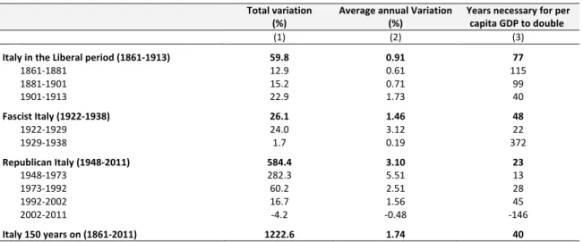
Having gone through the dynamics of per capita GDP levels, we now need to look at the rate at which it increased (or decreased) in the various periods considered. The calculations required – concerning GDP growth rates – are reported in Table 1. The first growth rate given in the table (column 1) refers to the overall change in GDP in each sub-period. This is a useful figure in that it tells us the magnitude of the change observed between the initial year and final one, but not very useful when we wish to compare periods of different lengths: it is clear that longer observation periods will tend to show greater total change rates. The problem is easily solved by calculating the annual percentage change (rather than the total one) during the period (column 2). The table also includes a third, alternative measure of the GDP growth rate: in column 3, instead of using the change rate, we calculated the number of years it would be necessary to wait before GDP doubled, assuming that it changes at a constant rate from one year to the next, that is, variations of the same percentage (the one given in column 2) every year5.
5 The calculation is based on a little rule known as the “rule of 70”, according to which the number of years
needed to double a certain magnitude can be calculated as the ration between 70 and the annual growth rate of the economic magnitude concerned. For example, if GDP grows at 2% a year, the formula tells us that we need to wait 35 years (= 70/2) before it doubles.
Table 1. The changeable rate of per capita GDP, Italy 1861-2011.
Total variation (%) Average annual Variation (%) Years necessary for per capita GDP to double
(1) (2) (3)
Italy in the Liberal period (1861-‐1913) 59.8 0.91 77
1861-‐1881 12.9 0.61 115 1881-‐1901 15.2 0.71 99 1901-‐1913 22.9 1.73 40 Fascist Italy (1922-‐1938) 26.1 1.46 48 1922-‐1929 24.0 3.12 22 1929-‐1938 1.7 0.19 372 Republican Italy (1948-‐2011) 584.4 3.10 23 1948-‐1973 282.3 5.51 13 1973-‐1992 60.2 2.51 28 1992-‐2002 16.7 1.56 45 2002-‐2011 -‐4.2 -‐0.48 -‐146
Italy 150 years on (1861-‐2011) 1222.6 1.74 40
The table compares per capita GDP growth rates for various periods of Italy’s post-unification history. Column (1) shows the total variation recorded during each sub-period (e.g., between 1861 and 1913, per capita GDP rose on the whole by 59.8%); column (2) shows average annual variation (e.g., between 1861 and 1913, per capita GDP rose at a rate of 0.91% per year); column (3) shows the number of years needed for per capita GDP to double, assuming that it changes at the average rate given in column 2 (e.g., given that the average annual growth rate between 1861 and 1913 was 0.91% per year, per capita GDP would take 77 years to double). The negative value observed in the last decade is interpreted as the number of years necessary for per capita GDP to halve.
If we wish to schematically summarise the main “facts” emerging in Table 1, then we could draw up the following list.
– 1861-1901. The first two generations of Italians in post-unification Italy did not experience high growth rates in per capita GDP. Indeed, the rate at which GDP increased over the first four decades of the new Kingdom of Italy (0.6-0.7% per year) would have required at least a century to double.
– The political unification of the country did not lead to any “take-off” with regard to the average income of its citizens, but to a slow and gradual increase6. However, something changed at the dawning of the twentieth century.
– 1901-1913. The years of the so-called “Giolitti age” saw an acceleration in GDP: compared to the previous two decades, the economic growth rate more than doubled (1.7% per year). World War I marked a sharp break in this favourable period, but growth would resume rapidly once again in the aftermath of the Treaty of Versailles (1919).
– 1922-1938. The new estimates describe the inter-war period as the combination of two decades that were very different from one another: the 1930s were as bleak (average per capita GDP growth rate was +0.2%), as the 1920s were rosy (+3.1%). Such a marked difference between the two decades constitutes a novelty not found in the previous literature.
– 1948-2011. The republican period shows features that are largely well known: (a) in the years 1948-1973 Italy sped along at an unprecedented rate it has not experienced again since (+5.5% per year); (b) The slowdown in the years 1973-1992 is very conspicuous: much like a motorist shifting from a cruising speed on an open highway
6 Toniolo (2013) gives two reasons for the deadlock of this period. On the one hand, there was the
sluggishness (a) of the process for creating a single national market (political, administrative and economic unification did not come about overnight), (b) of the formation of an adequate human capital stock (schooling of the population was difficult) and (c) in the establishment of the new legal institutions (from the single currency to the approval of the commercial and administrative codes). On the other hand, there were external shocks (two wars of independence, the problem of banditry in the south of the country) and economic policy mistakes with regard to trade and monetary matters.
to a much slower pace on entering a town; (c) in the last decade (1992-2011), per capita GDP actually fell by 0.5% per year.
Box 3 – A very long-term look, Italy 1300-2011.
Our curiosity of knowing the average income of the Italians in the centuries preceding the country’s unification may, at least in part, be fulfilled. Economic historians have actually estimated GDP even for unsuspectingly remote times. The most adventurous estimates refer to the Ancient Roman period: according to Maddison (2007), at the time of the death of Emperor Augustus (14 DC), the Italic peninsula was (by far) the richest of all the Roman provinces of the Mediterranean basin. Instead, the following centuries were, on the whole, bleak and characterised
by a long period of decline, with signs of recovery found only around the 10th century [Lo Cascio
and Malanima 2005: 204-5].
The earliest reliable estimates for per capita GDP of the Italian peninsula date back to 1300: by connecting the reconstruction made by Malanima (2006) to the new estimates of the period 1861-2011, we obtain the curve shown in the figure above. This reveals the distinctive features of a pre-industrial economy, that is, a centuries-old stagnation of per-capita GDP. The graph’s scale hides as much the frequency as the intensity of the annual variations: although the Italian economy of the early Middle Ages had a mastery of the most advanced technology of the times [Cipolla 1952], there were recurring famines, even within the same generation [Livi Bacci 1991: xx; Malanima
0 5000 10000 15000 20000 PI L PER ABI T AN T E (1 9 9 0 PPP U SD ) 1300 1350 1400 1450 1500 1550 1600 1650 1700 1750 1800 1850 1900 1950 2000 ANNO
The graph shows the trend in per-capita GDP (vertical axis) over time (horizontal axis). The stationariness observed from the 14th century to the 19th century corresponds to the pre-industrial economy; modern economic development started in the latter half of the nineteenth century.
2003], with disastrous consequences on the population’s standard of living [Ò Grada 2009].
With the start of the Modern Age, say from 1500, the overall GDP of the Italian economy started to rise, but it was accompanied by an even greater increase in the population, with the result shown in the figure: a slow but inexorable decline in per-capita income [Malanima 2006: 21]. Despite this downward trend, Italy is still considered to have been one of the most advanced countries until the mid-1700s. After this time, the gap with other western European countries started to increase: “Things changed after 1750. For more than a century, with very short interruptions, the Italian economy experienced a decline which was at once absolute and relative.” [Malanima 2006: 111]. As we know, at the close of the 1700s Italy missed out on the first industrial revolution, not being able to adopt British technology based on steam and the railways [Allen 2009]. This is reflected in the GDP trend in the figure, which shows a flat trend in continuation of the past. The curve starts to rise in the last decades of the nineteenth century, during the second industrial revolution, based on electricity, oil and chemicals [Mokyr 1990]. This marks an epochal moment in the history of the wellbeing of the Italians – a crossroads in history where Italy took the right road and embarked on the process of “modern economic development” described by Kuznets [1966]: rural backward Italy embarked on a deep transformation which would change its features, on both a qualitative and quantitative level, and turn it into an advanced economy within the space of a century or so.
5. Interpreting the past
Right from World War II, historiographers have put forward various, often conflicting, hypotheses to explain the country’s industrialization and modernization process, summarized in the long-term trend of per-capita GDP (figure 1). In this section, we shall segment Italy’s per-capita GDP series into the three periods corresponding to the political periodization of the country over the 150 years since its unification: the Liberal period (1861-1913), the Fascist period (1922-1938) and Republican Italy (since 1946). We shall
thus examine each phase in sequence, placing the GDP series within a broader context in which we shall introduce, albeit superficially, the technological progress and institutions – two key factors to explain a country’s long-term economic performance.
Technology is behind increases in productivity and thus represents the main determinant in per-capita GDP [Jovanovic and Rosseau 2005; Giannetti 2001]. Over the 150 years since its unification, Italy has gone through as many as four technological regimes [Freeman and Perez 1988]: (a) the first (1861-1875) is the one identified by the three main inventions of the times, the steam engine, the spinning machine and the railways; (b) the second (1875-1908) coincides with the “second industrial revolution”, characterized by heavy industry (steel, first and foremost, to which the mechanical industry is connected) and electricity; (c) the third (1908-1970s) is defined by the establishment of mass production, such as with Henry Ford, in which petroleum plays a key role and there is the take-off and affirmation of durable consumer goods, starting with the automobile; (d) the fourth and last regime corresponds to the “third industrial revolution” (1970s-today) triggered by the advent of information technology and telecommunications: the industries showing the fastest growth in this phase are linked to electronics and particularly to computer technology [Gordon 2012]. The dates marking the shift from one regime to another are obviously approximate and only serve to outline the timeline with which the main innovations have followed on from one another.
Technology represents a necessary but not sufficient condition for a country to feed its own course towards prosperity: the technological changes must be accompanied
by changes in the institutions, in the broadest sense, and in the society’s ideology7. Did the new technological paradigms – exogenous factors with regard to the Italian economy – find fertile terrain in the country owing to the fact that institutions and ideologies were favorable to their adoption?
5.1 The industrialization of the peninsula (1861-1913)
Much has been written on the economic history of Liberal period Italy8. The question at
the heart of the historiographic debate has often been the following: when and why – from being a rural country, “poor” and backward, as it had been for centuries – did Italy become an industrial country, “wealthy” and modern? The “giant who dominated the Italian debate” after World War II was Alexander Gerschenkron (1904-1979), a US-naturalized Russian economist; it is worth starting from his thesis [Fenoaltea 2007: 352]. Gerschenkron identified the “big industrial push” of the country around the mid-1890s and put it down to the creation of mixed banks – Banca Commerciale Italiana (Comit), founded in 1894 with German capital, Credito Italiano (Credit), Banco di Roma, and later on Banca Italiana di Sconto. Mixed banks, or universal banks, are so called because they collect capital (the prerogative of commercial banks) and channel it to favor industrial development (the prerogative of investment banks). Through their network of branches, mixed banks collect deposits short-term from ordinary citizens to then invest the capital in shares: that is, they turn the capital into long-term credit to industry:
7 This is a fundamental point in the speech Simon Kuznets made in Stockholm when he received the Nobel
prize for economics [Kuznets 1971], taken up again in various forms by Abramowitz (1986), and more recently by Acemoglu and Robinson (2012). See also Felice and Vecchi (2013).
8 Among the more important recent monographs, see Toniolo (1988, 2012), Zamagni (1993), Fenoaltea
precisely what is needed, according to Gerschenkron, to favor the industrialization of a backward country.9 For Gerschenkron, this was the institutional innovation that acted as the “engine of growth”, in Italy and in Germany: it was the mixed banks which managed to compensate for the country’s drawbacks (the scarcity of natural resources, the political instability and hesitations of governments during the first decades after unification, the insipience of economic policies) on the path toward Italy’s industrialization [Gerschenkron 1955, 1959 and 1962].
The debate following Gerschenkron’s work was intense and remained so over the following decades. The common denominator of all the interpretations put forward in the successive years was that of assuming that economic development followed a stage-by-stage model [Rostow 1960]. According to this view, a country develops following an orderly sequence of stages (or phases). Initially, the prerequisites for growth must be created (for instance, infrastructure and human capital); the second stage envisages an economic take-off – economic growth starts up with a great boost and marks a break with the GDP series trend; the next stage marks a rise to maturity (technology opens up new investment opportunities and the economy becomes more complex), and, finally, there is the age of mass wellbeing.
9 In return, the mixed banks typically entered the boards of the firms they financed and obtained access to
strategic information. The advantages associated with the presence of a mixed bank must be weighed up against the greater fragility of the economic system, due to the interweave that is created between credit capital (banking system) and industrial capital (the real economy).
Figure 2. Per-capita GDP between 1861 and 1913: no lull, no take-off
III guerra indip.
PIRELLI (gomma) Sinistra storica
Protezionismo
Scandalo bancario
Inizio età giolittiana
Guerra di Libia
BARILLA (alimentare)
FIAT (auto)
OLIVETTI (macchine da scrivere)
EDISON (elettricità) TERNI (acciaio) FALCK (acciaio) BREDA (meccanica) MONTECATINI (chimica) 2000 2500 3000 3500 PI L PER ABI T AN T E (e u ro 2 0 1 0 ) 1861 1871 1881 1891 1901 1911 Anno Motore a vapore e ferrovie Acciaio ed elettricità
Motore a combustione interna, petrolio, produzione di massa
The figure shows the per-capita GDP trend against the background of technological changes (indicated with a different background color intensity), and the main political and economic innovations.
It is difficult to establish whether the per-capita GDP series in figure 2 shows a trend in line with the explanation offered by stage-based models. The first two decades of post-unification Italy show an uncertain start, and it is only with the beginning of the “Historical Left” and the Depretis Government (1876) that GDP started to grow at an increased rate. The trend does not show any trace of the crisis of the 1880s, while the slowdown in the 1890s is well visible. On the whole, the terms “take-off” or “big industrial push” are quite inappropriate to describe the trend with regard to the latter half of the 1890s.
An alternative interpretation to the one suggested by the stage-based model was proposed by Fenoaltea [1988, 2006]. In this case, the story begins by observing that the new GDP series has an upward trend with no breaks or take-offs, but with fluctuations:
these are “economic cycles”, mainly caused by the construction industry and more generally by the infrastructure sector. According to Fenoaltea, construction and infrastructure were in turn driven by foreign investment, especially British at the time: therefore, what decided the various stages of Italian economic growth during the Liberal period was the foreign investment cycle. In this model, Italy behaves like any other European fringe country: when the political climate positively influences investor expectations, capital flows in and the economy gets going; when greater risk is perceived, capital flows cease, indeed, they flow out of the country and the economy contracts. The view of Italy as an “open economy”, that is to say, as part of an international economic system, does not require any stage-based development process and does not envisage any take-off stage: the process is guided by the interweaving of the international economic cycle, investor expectations and the domestic political cycle. Fenoaltea’s interpretation appears largely consistent with a cyclical development along an increasing trend, as the one shown in figure 2. Less convincing is the fact that it overlooks the role played by national institutions and domestic economic policy decisions10. This point has been grasped and well reasoned out by Gianni Toniolo:
In order to profit from the international boom, Italy had to abandon expensive colonial adventures and put order to its public finances, rebuild almost from zero a banking system that laid in tatters, create a central bank, overcome the credibility shock generated by the suspension of gold convertibility. More than that: Italy had to overcome a social and political
10 See Toniolo (2012). On a more technical level, we may add the following observation: the estimates by
Felice and Carreras (2012) with regard to just industry for the period 1911-1951, when combined with those of Fenoaltea (1861-1913), suggest that the cyclical model is valid only up to the mid-1890s. From that time on, more or less coinciding with the creation of the mixed banks, for the cycle of Italian industry not only does the production of durable goods count, but also the production of consumer goods.
crisis that threatened to undermine the very foundations of the liberal state. Both politics and society stood up to the occasion: the crisis (...) was overcome. Democracy was maintained, the disastrous African policy was discontinued, sound economic institutions were put in place and the banking system was revitalized. In the following years successive governments maintained a time-consistent fiscal and monetary policy, the gold standard was shadowed but cleverly not officially reinstated, commercial treaties brought back the fresh air of freer trade. All this lies behind Italy’s ability to surf the long wave of international growth. It did not
need to be so: even sailing with the tide requires expert skippers. [Toniolo 2007, p. 132. Our
italics]
5.2 The interwar period (1919-1938)
Compared to the Liberal period, the interwar years have received a lot less attention11.
This is certainly a bad thing because it was a decisive period in which Italy modernized and enhanced the sectors of the second industrial revolution (chemicals and heavy industry at the expense of textiles and foodstuffs), and also saw progress at the institutional level by creating the foundations which would accompany the subsequent economic miracle.
Even though it was a rather difficult time, to say the least, at a domestic level and even more so at the international one (two world wars, the Great Crisis of 1929, the Fascist dictatorship and its autarchic turn), in the period 1919-1938 the per-capita GDP growth rate (1.5% a year) was significantly higher than the one recorded during the Liberal period (0.9%).
11 Among the exceptions: Toniolo (1980), Gualerni (1995), Galimberti and Paolazzi (1998), Petri (2002),
Behind this overall figure lie very diverse trends which characterized the 1920s and 1930s (figure 3). The growth of the 1920s was rapid, the result of an increase in productivity; if the war had any beneficial consequence, then it was its positive effect on the technological backwardness accumulated during the conflict – technological progress in the chemical industry, in motor vehicle production and in aeronautics was greatly stimulated by the war effort [Feinstein, Temin and Toniolo 1998: 87]. Between 1919 and 1929, Italy grew at a high rate – over 3% a year, on average. The 1920s were really “Roaring Twenties” for the Italians, but these were then followed by very difficult years economically, and even more so politically, speaking. The Great Depression of 1929 appears to have had a greater impact than previously thought: between 1929 and 1933 Italy suffered an 8% decrease in per-capita GDP compared to the 3.5% decrease previously estimated by the “old” series [Vitali 1969]. This is higher than the UK figure (-4%), close to the French (-10%) and German (-12%) ones, but a long way off from the catastrophic figure recorded in the USA, where GDP decreased by 27%.
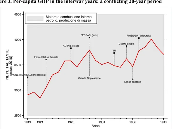
Figure 3. Per-capita GDP in the interwar years: a conflicting 20-year period
MAGNETI MARELLI (meccanica)
Grande Depressione
IRI
Guerra Etiopia
Legge bancaria Inizio dittatura fascista
AGIP (petrolio) FINSIDER (siderurgia) FERRARI (auto) 2500 3000 3500 4000 4500 PI L PER ABI T AN T E (e u ro 2 0 1 0 ) 1919 1921 1926 1931 1936 1941 Anno Motore a combustione interna, petrolio, produzione di massa
The interwar period was characterized by very marked economic cycles: the graph shows a boom in the decade after the Treaty of Versailles (1919-1929), the recession following the 1929 crisis and the lively recovery starting in the latter half of the 1930s.
Paradoxically, but perhaps not so much, it was the very autarchic policies which steered modernization and thus the expansion of the Italian productive base: the deflationary turning point of 1926 (with the drastic revaluation of the Italian lira) made the price of imported materials (e.g. cast iron) and of machinery drop, thereby benefiting industry which could use inputs at lower prices. At the same time, however, it made prices rise for traditional Italian exports in light industries such as textiles, thereby damaging the less advanced Italian production sectors. The 1929 crisis led to a broad reform of the Italian production system. On the one hand, it forced the industrial sector to substitute labor
(now more expensive12) with capital, and this led to an increase in mechanization; on the other, the calamitous effects of the crisis on the real economy and on finance led to the institutional reorganization of the whole edifice of national capitalism. The institute for industrial reconstruction IRI (Istituto per la Ricostruzione Industriale) was created in 1933, and in 1936 the banking reform law achieved the separation between banks and industry, that is, between short-term and long-term credit.
On the whole, the prevalent view today in interpreting the interwar period is that the Fascist years were not a break in the long-term path of the Italian economy, but rather a premise for the great leap which would take place after World War II [Gualerni 1995; Petri 2002; De Cecco 2000].
5.3 From the periphery to the centre (1946-2011)
The new GDP estimates (figure 4) for the years following World War II do not add very much to what we already knew. Once post-war reconstruction was completed, Italy “put on wings” and embarked on a period of growth which history would call the “economic miracle”13. The new estimates confirm the exceptional performance of the 1950s and 1960s which emphasize – as we saw in Box 4 – an actual break in the centuries old trend [Malanima 2003; 2006]. It is these two decades which saw Italy complete its transition from the “periphery to the centre”, according to the fortunate definition put forward by
12
Deflation, i.e. price decreases, led to a rise in real wages, or to an increase in the labor factor of production, which became more expensive compared to other goods [Mattesini and Quintieri, 1997].
13 In actual fact, GDP showed a miraculous trend in most countries in western Europe: not surprisingly, the
Vera Zamagni [1993]: the country became a modern industrial one, with a great shift in labor from rural areas to industry, even in Italy’s Mezzogiorno or southern regions. There were many reasons for this achievement, starting from some decisions in the geopolitical and international arena. Firstly, the Marshall Plan, whose funds were used better in Italy (to renovate the industrial apparatus) than in other countries [Zamagni 1997; Fauri 2010]. Secondly, the far-seeing anchorage to the European edifice [Fauri 2001; Ciocca 2007]. Other factors also moved in the right direction. The fixed exchange rate system based on the dollar, low prices for oil and other natural resources, the gradual liberalization of international trade brought their benefits to more or less all advanced countries, and particularly to Italy: for example, the decrease in raw material prices in the 1950s and 1960s was particularly advantageous for a country lacking in natural resources.
Among the important elements explaining the country’s growth after World War II there is also the continuity with the past, and particularly with regard to the interwar years. This is the case with the system of partecipazioni statali (that is, of enterprises indirectly owned by the state through management entities), which was created in the 1930s and made an important contribution to growth in the 1950s and 1960s, becoming the driving force of industrial modernization. There is no counter-evidence, obviously, but the idea which has been put forward is that these state holdings played a key role making it possible to devise “far-seeing strategic plans which were instead absent – if we exclude FIAT of Valletta – in large scale private industry” [Barca and Trento 1997: 197]. By the end of the 1960s, Italian industry appeared broadly diversified and even impressive, in some respects: the country excelled in the automobile and IT sector, developed an important chemicals industry and was at the forefront of the aerospace industry. At the same time, there were also those traditional sectors of made in Italy
(particularly textiles, footwear, food and home furnishings), supported by a widespread fabric of small and medium-sized enterprises [Amatori, 1980, 2011; Colli and Vasta, 2010].
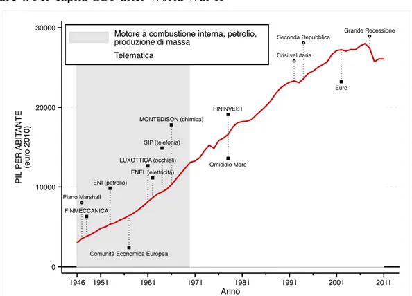
Figure 4. Per-capita GDP after World War II
Piano Marshall FINMECCANICA LUXOTTICA (occhiali) ENEL (elettricità) SIP (telefonia) MONTEDISON (chimica) Crisi valutaria Seconda Repubblica FININVEST Grande Recessione ENI (petrolio)
Comunità Economica Europea
Euro Omicidio Moro 0 10000 20000 30000 PI L PER ABI T AN T E (e u ro 2 0 1 0 ) 1946 1951 1961 1971 1981 1991 2001 2011 Anno Motore a combustione interna, petrolio, produzione di massa
Telematica
GDP in the decades after World War II is characterized by an upward trend – taking Italy from the “periphery to the centre” – and by a conspicuous slowdown starting in the 1990s, leading to stagnation with the advent of the new millennium.
Growth slowed down in the 1970s and 1980s, starting with the first energy crisis in 1973: the system of partecipazioni statali degenerated and ended up by obeying clientele-type political demands which led to setting up manufacturing plants in locations that were far from convenient [Felice 2010]. Large scale enterprises lost ground and a tertiarization of the economy – that is, a GDP shift from industry to services – took hold in Italy, too.
In any case, the GDP increase in this period still appeared in line with that of the main European competitors, driven by exports and by the country’s industrial districts14. The latter seem to take on a new paradigm in the history of enterprise, but some critical observers [De Cecco 2000] noted how their rise owed more to the devaluation of the lira and to a lack of fiscal control: a view confirmed in the light of their disappointing performance in recent years.
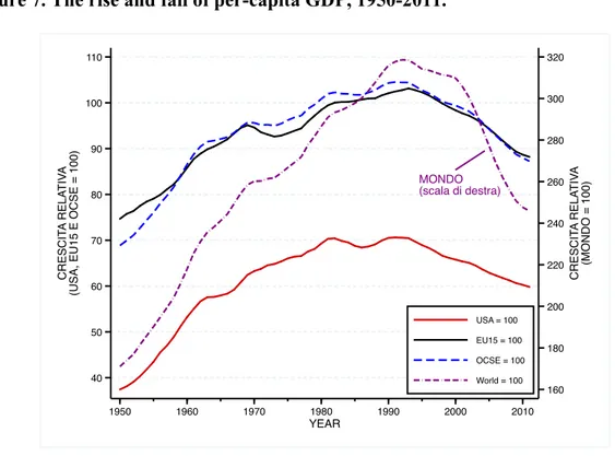
The years since 1992 have witnessed a decrease in growth, more than halving even with respect to the previous twenty-year period. As Salvatore Rossi (2010) observed, “Adapting to the ICT revolution and globalization (…) was, and is, not an easy operation, above all with regard to the change in technological paradigm.” (p. 15). What has characterized the last twenty years is, in sum, a hitherto unprecedented inability to adapt to the context – once again exogenously given – that Italy has to operate in [Paolazzi and Sylos Labini 2012]. Italy has fallen behind, and visibly so, compared to its main European partners, which in turn have lost ground to the USA and even more to emerging Asian countries (we shall see this in section 7). At the turn of the millennium, both the national press and public opinion spoke in terms of an economic decline (Box 4).
14 An industrial district is a system of highly specialized small and medium-sized enterprises geared to
export and active in a specific geographical area providing them with the necessary social and economic infrastructure. In synergy with other local institutions, these firms manage to cut transaction costs without requiring a hierarchical structure that is typical of large enterprises [Becattini 1979].
Box 4 – Words are important: recession and depression, crisis and decline.
Recession, crisis, depression and economic decline. These are the words that begin to circulate as soon as GDP slows down. If the media do not always pay the necessary attention to them, there are important
differences between their everyday
meaning and their technical one. It is worth going into their meaning, not for the sake of semantics, but as a premise in order to more clearly deal with the theme of Italy’s economic decline.
Recession. In everyday language, periods of positive growth in GDP are called “expansions” while
periods of negative growth are called “recessions” (or “contractions”); alternating periods of expansion and contraction of GDP give rise to the so-called economic cycle. In economics, the word recession is only used when the period of negative growth lasts at least two consecutive quarters [Blanchard 1997: 25]. There is an alternative definition, used by the US National Bureau for Economic Research (NBER), that, unlike the previous definition, is also sensitive to the scale of the GDP decrease (the idea is that it is worth distinguishing between a 0.1% decrease and a 10% one) and depends not only on the GDP trend, but also on that of other indicators (such as unemployment or sales volume). According to the NBER, “a recession is a significant decline in economic activity spread across the economy, lasting more than a few months, normally visible in real GDP, real income, employment, industrial production, and wholesale-retail sales” [NBER 2008]. In practice, the two definitions often coincide, but not always and not necessarily so.
Crisis. There is no single technical or formal definition of the word “crisis”. Ironically, the most
prestigious Italian encyclopedia, published by the Istituto Treccani, discontinued the volume containing the entry “economic crises” in 1931, right at the height of the most serious crisis of the capitalist economy. The definition underlined the element of surprise and the speed associated with
An illustration (still in preparation) by Roberta Zanetti, inspired by the front cover of The Economist of 16 July 2011.
the phenomenon: “The crisis is a shift, often a sudden one, from a given equilibrium position to another very different one; the shift is usually a jolting one and unexpected by many of the agents, and brusquely leads to serious decreases of value and of production activity, a reduction or cessation of remuneration; it is often accompanied by bewilderment, by dramatic episodes.” (p. 913, our italics). Since then the international specialist literature has tended to replace the generic term “economic crisis” by distinguishing between a financial crisis (linked to monetary, banking and exchange-rate matters or to the public debt) and a crisis concerning the real economy. Carmen Reinhart and Kenneth Rogoff (2011) defined the various forms of crisis in quantitative terms: although it is still a little too early to consider the definitions proposed by the two authors as a “standard”, they are, undoubtedly, the most authoritative we have available today.
Depression. Likewise for the word “depression”, economists still do not have a univocal definition.
The new edition of the Palgrave Dictionary of Economics has even removed this entry, while the previous editions attributed an international dimension to the term that is totally missing in the definition of recession: “That term [depression] is reserved for longer periods of more serious adversity on an international scale” (ed. 1987: p. 809). John Maynard Keynes provided an implicit definition of depression: “a chronic condition of subnormal activity for a considerable period without any marked tendency either towards recovery or towards complete collapse” [Keynes 1936:
cap. 18]. More recently, Paul Krugman (who won the 2008 Nobel prize for economics) put forward
an informal, but very practical, definition of the term: “depression” describes a situation where the
normal medicines (the economic policy tools) administered to the system in order to boost economic activity do not work [Krugman 2012]. In short, an economic system would be in a state of depression as soon as economists have repeatedly shown they do not know what to suggest to trigger a recovery.
Decline. Attempting to say what “economic decline” should be taken to mean in the space of a few
lines is the hardest task. On the topic of decline, the most interesting reflections are undoubtedly the ones found in economic history. Gianni Toniolo (2004) wrote an essay full of reflections from which we can gather the features of an economic decline: (1) we must distinguish between an
past) and relative decline (when a country cannot keep up with the most dynamic economies and, although not experiencing any actual worsening of living conditions, goes down in the international ranking of prosperity); (2) a decline has many facets: it concerns the economy, but it is the symptom of a more general malaise involving the institutions, politics, society and culture, that turns into sclerosis, into a loss of vitality, and into a recalling of past models [p. 22]; (3) a decline is slow and hardly perceptible: it becomes a political and social problem only when its effects are very widespread and the cost of ignoring them becomes unbearable for the governing elite, sometimes due to shocks such as wars, revolutions and great financial crises [p. 10]; (4) about the causes, a decline stems from the inability to adapt an old production model to new circumstances, and this inability to adjust is greater the more successful the older model had been in the past [p. 9].
6. At last, the GDP of the regions
Once Italy’s national accounts had been reconstructed, some economic historians began to pursue the aim of replicating the task for each one of the Italian regions. The first attempt on this was made by Vera Zamagni in 1978 by drawing up an income estimation of the Italian regions for the year 1911. Although she was successful, hers was an isolated attempt: silence soon returned and in the next two decades the measurement of regional differences in GDP remained a poorly researched field15. The new millennium heralded new studies enabling, at last, an outline of long-term per-capita GDP development for each of the country’s regions. The summary picture we offer in this section is a useful, if not indeed essential, premise for understanding the origins of territorial imbalances today.
15 Official statistics on regional GDP only started to be published in 1970 [Svimez 1993]. Esposto (1997)
produced estimates for 1971 (macro-regions), 1891 and 1911; Svimez [1961] for 1938 and 1951; Daniele and Malanima [2007, 2011] produced annual estimates from 1861 to 1951, by bringing together estimates made by Federico [2003b], Fenoaltea [2003b] and Felice [2005a, 2005b], in the assumption that, for each sector of economic activity (agriculture, industry or the services), the regional cycles would be the same as the national cycle. This section is based on Felice (2011) and on hitherto unpublished estimates for 1871 and 1931.
The trend of regional differences in per-capita GDP for the five large macro-areas of the country is summarized in figure 5. There are three very interesting results and they deserve a brief comment. The first concerns the so-called baseline conditions. In our baseline year (1871), Italy showed non-negligible per-capita GDP differences: the richest area of the country, the North-West, had around a 25% advantage over the poorest area, the South (about 2,000 Euros per person a year in the North-West versus 1,600 Euros in the South). This is a significant difference, consistent with what emerges in other chapters of this book, considering other social indicators, and with what we know about the distribution of transport and credit infrastructure, which point to a clear advantage for the northern regions [Zamagni 1993: 42; Giuntini 1999b: 597]. In order to interpret these differences properly, we must also not overlook the fact that, in 1871, Italy as a whole still had to face the great industrial transformation – the only change that could decisively raise income levels. The situation in other countries was rather similar: new data for Spain [Rosés, Martínez-Galarraga and Tirado 2011] or for the Austria-Hungarian empire [Schulze 2007] indicate a gap in favor of regions with an industrial or services base – Madrid and Catalonia, in the former case, and Vienna, in the latter – but, on the whole, also a relatively modest dispersion of average incomes compared to what would happen as industrialization progressed.
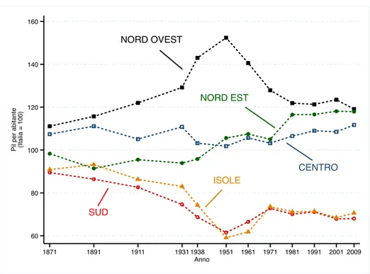
Figure 5. The great Italian divide, 1871-date. NORD OVEST SUD NORD EST CENTRO ISOLE 60 80 100 120 140 160 Pi l p e r a b ita n te (I ta lia = 1 0 0 ) 1871 1891 1911 1931 1938 1951 1961 1971 1981 1991 2001 2009 Anno
The graph shows the per-capita GDP trend (measured along the vertical axis, with Italy = 100) for each macro-region of the country. The long-term trend shows a process of divergence which is interrupted only
in the years 1951-1971. The definition of the macro-regions is provided in map X on page Y.
A second comment concerns the spectacular long-term divergence process: the North-West regions start from slightly more advantageous baseline conditions, but then proceed at such a pace that in the aftermath of World War II they are a “world apart”: in 1951 the citizens of the north-western regions would enjoy a 50% higher GDP than the national average. The southern regions, instead, show a diametrically opposite trend, falling behind the rest of the country, such that in the aftermath of World War II they become a sort of second Italy: per-capita GDP in the south is less than half the one of the central-northern regions.
Once again, if figure 5 would not surprise historians – the southern question has been on the scholars’ table since the last century – what remains striking is the sheer
scale of these differences. It is the actual amounts emerging in figure 4 that are stunning:
in 1951, after 90 years of post-unification history, the southern regions had a per-capita GDP of 2,860 Euros a year at today’s purchasing power parity (table X in the statistical appendix), a value accounting for barely 40% of the north-western regions (where per-capita GDP was 7,180 Euros a year). The average income in Calabria was less than a third (29%) of the one in Liguria.
The third result deserving particular attention concerns what occurred in the interwar years: regional differences increased conspicuously. In this period the North-West progressed along the path of industrialization and modernization, while the
Mezzogiorno remained dramatically still16. A factor favoring development in the North-West was the country’s great effort in World War I (1915-1918) which steered public procurement towards enterprises of the so-called “industrial triangle” (Lombardy, Piedmont and Liguria), the only ones that could deal with the production demands of the war. The north also benefited from deflationary measures and an autarchic policy (section 5.2) which meant an intensification of industrial production towards advanced sectors, mostly located in the north. Instead, the Mezzogiorno suffered from the demographic policies of the Fascist regime, with restrictions to emigration (chapter Z Migration), and this increased the demographic pressure on the poorest regions. To this must be added the effect of the so-called “wheat battle” (in 1925 Mussolini proclaimed the need for Italy to achieve self-sufficiency in food, starting with wheat), which favored cereal growing at the expense of more profitable crops of Puglia and Sicily (wine, grapes and citrus fruits),
16 This can be illustrated by the following data: between 1911 and 1951, the percentage of agricultural labor
in southern Italy did not decrease (remaining at around 60%), while in the north-west of the country, in the same period, it fell by almost 20 points from 47% to 28% [Felice 2011].
and the immobilism of the social order that guaranteed the rents of great landowners even when the land itself was not productive, thereby hindering modernization in southern agriculture [Bevilacqua 1980; Felice 2007a].
Regional differences greatly decreased from 1951 to 1971. Convergence of the south during the 1950s and 1960s was exceptional and made possible both by the start-up of considerable inter-regional migration from south to north of the country as well as by a
deus ex machina – the great public sector intervention. The Cassa per il Mezzogiorno (the
Southern Italy Development Fund), set up in 1950, was the instrument through which the State promoted the creation of great infrastructural works in the southern regions – from aqueducts to roads and industrial plants. As well as direct intervention for creating the necessary infrastructure, the Cassa also provided for indirect funding of production activities. The initiatives involved public enterprises, which were obliged by law to devote a considerable amount of their investment to the Mezzogiorno, but also private ones: both kinds of enterprises received lower interest rate loans and free contributions. It was a top-down action focusing on “heavy”, higher added value sectors such as the chemical, steel and advanced mechanical industries17. In terms of resources allocated in relation to GDP, the investment was on a scale unparalleled in any other western European country [Felice 2002].
This convergence of the Mezzogiorno turned out to be short-lived, however: the economic policy was not enough to trigger a continuous self-generating process in the south. With the oil crisis of the 1970s, the Ford model based on large energy-intensive factories suffered a setback, and in Italy this was particularly felt by the weaker links of the chain, that is, the plants in southern Italy that had been located there not for market
convenience, but because of State incentives or dispositions. At this point, public intervention showed itself to be incapable of reinventing itself and indeed became entangled in a great many welfare or income support trickles, bloating the staff of public administrations and even benefiting organized crime18.
Figure 5 clearly shows that from the 1970s onwards, albeit slowly, the southern regions started to fall behind again. The north-eastern regions instead started to pick up pace in their convergence with the north-western ones, followed by the central regions of the country. The driving force of the north-east was a growing capillary network of export-geared manufacturing firms [Bagnasco 1977; Becattini 1979]. The most recent data, of 2009, confirm broad gaps – broader than the ones estimated for the time of Italy’s unification. As we shall see better in the next section, economic integration made no real progress19.
7. Divided at the middle
Exactly ten years after Simon Kuznets hypothesized an upside-down U-shaped curve for the relation between income inequality and economic growth (Chapter 10, Inequality), the economic historian Jeffrey Williamson proposed another upside-down U-shaped curve, this time to describe the trend in the regional income inequalities within the same country [Kuznets 1955; Williamson 1965]. Kuznets had concerned himself with the
18 See Bevilacqua (1993: 126-7, 132) and Trigilia (1992). The Cassa per il Mezzogiorno was dissolved in
1984.
19 Per-capita GDP differences between the various geographical macro-regions concerned could be
explained by the price differences found in these areas (Chapter 11 Cost of Living). This is not the case here. Brunetti, Felice and Vecchi (2011) showed that by correcting GDP to allow for differences in purchasing power does not change the key features of the historical picture described in figure 5.
distribution of benefits of economic growth in the population while Williamson was interested in the sequence with which the various areas of the country managed to bridge the gap with the most successful regions. “Economists have long recognized the existence and stubborn persistence of regional dualism at all levels of national development and throughout the historical experience of almost all presently developed countries”, observed Williamson (1965: 3). Despite this awareness, however, a convincing explanation for this empirical regularity had still not been found; on the contrary, “one only needs to observe that Frenchmen, Italians, Brazilians, and Americans still tend to treat their North-South problems as unique to their own national experience with economic growth” [Williamson 1965: 3]. What must we expect, then, in the course of economic development? The income convergence of regions? If so, in what way and at what pace? If not, why not? Williamson answered by hypothesizing an upside-down U-shaped curve: (a) regional inequalities increase in the first stages of industrialization, when the nascent industries tend to concentrate in certain regions rather than in others, and (b) they decrease over the following decades owing to a series of mechanisms (labor and capital flows as well as the national government’s economic policy actions) which favor the spreading of industrialization in the country thereby redressing income disparities between regions. The analysis made in this section shows that, in the Italian case, Williamson was right. At least, up to a point.
The empirical exercise we shall now illustrate consists of dividing the country into two parts: the centre-north and the Mezzogiorno (which we shall refer to as North and South for the sake of brevity). The territorial inequality observed at national level in a given year may be considered as the result of two very different phenomena: 1) on the one hand, there may be great inequality in per-capita GDP within each area (for example,