PROCEEDINGS OF ECOS 2015 - THE 28TH INTERNATIONAL CONFERENCE ON
EFFICIENCY, COST, OPTIMIZATION, SIMULATION AND ENVIRONMENTAL IMPACT OF ENERGY SYSTEMS JUNE 30-JULY 3, 2015, PAU, FRANCE
Use of Degree of Disequilibrium Analysis to
Select Kinetic Constraints for the Rate-Controlled
Constrained-Equilibrium (RCCE) Method
G.P. Berettaa, M. Janbozorgib, and H. Metghalchic
a Università di Brescia, Brescia, Italy, [email protected] b University of Southern California, Los Angeles, CA, [email protected]
c Northeastern University, Boston, MA, [email protected]
Abstract:
The Rate-Controlled Constrained-Equilibrium (RCCE) method provides a general framework that enables, with the same ease, reduced order kinetic modelling at three different levels of approximation: shifting equilibrium, frozen equilibrium, as well as non-equilibrium chemical kinetics. The method in general requires a significantly smaller number of differential equations than the dimension of the underlying Detailed Kinetic Model (DKM) for acceptable accuracies. To provide accurate approximations, however, the method requires accurate identification of the bottleneck kinetic mechanisms responsible for slowing down the relaxation of the state of the system towards local chemical equilibrium. In other words, the method requires that such bottleneck mechanisms be characterized by means of a set of representative constraints. So far, a drawback of the RCCE method has been the absence of a systematic algorithm that would allow a fully automatable identification of the best constraints for a given range of thermodynamic conditions and a required level of approximation. In this paper, we provide the first of two steps towards such algorithm based on the analysis of the degrees of disequilibrium (DoD) of chemical reactions in the underlying DKM. In any given DKM the number of rate-limiting kinetic bottlenecks is generally much smaller than the number of species in the model. As a result, the DoDs of all the chemical reactions effectively assemble into a small number of groups that bear the information of the rate-controlling constraints. The DoDs of all reactions in each group exhibit almost identical behaviour (time evolution, spatial dependence). Upon identification of these groups, the proposed kernel analysis of N matrices that are obtained from the stoichiometric coefficients yields the N constraints that effectively control the dynamics of the system. The method is demonstrated within the framework of modeling the expansion of products of the oxy-combustion of hydrogen through a quasi one-dimensional supersonic nozzle. The analysis predicts and RCCE simulations confirm that, under the geometrical and boundary conditions considered, the underlying DKM is accurately represented by only two bottleneck kinetic mechanisms, instead of the three constraints identified for the same problem in a recently published work also based, in part, on DoD analysis.
Keywords:
Model order reduction in chemical kinetics, Non-equilibrium thermodynamics, Rate-controlled constrained-equilibrium (RCCE) method, Chemical relaxation
1. Introduction
According to the Rate-Controlled Constrained-Equilibrium (RCCE) model reduction scheme, the reactions in a detailed kinetic mechanism (DKM) can be characterized in terms of the effectiveness with which they contribute to the spontaneous (irreversible, entropy generating) tendency to relax the composition towards chemical equilibrium. Loosely speaking, such effectiveness depends on the number of "kinetic bottlenecks" that the reaction needs to go through in order to advance and on how "narrow" these bottlenecks are. Each kinetic bottleneck is characterized by a linear combination of the composition, called a "constraint", which can be varied only by reactions that go
through that particular bottleneck. Therefore, the "narrower" the bottleneck, the slower the rate of change of the associated constraint.
The general idea behind the RCCE method [1-8] is that for each particular problem and set of conditions, there is a threshold time scale which essentially separates the fast equilibrating kinetic mechanisms from those that slow down and control the spontaneous relaxation towards equilibrium. The slow mechanisms control the interesting part of the non-equilibrium dynamics in that they effectively identify a low dimensional manifold in composition space, where, to a very good approximation, the dynamics can be assumed to take place. In general these rate controlling mechanisms are slow because they have to go through one or more bottlenecks. For example, the three-body reactions are slow because they require three-body collisions which occur much less frequently than two-body collisions. As a result, the bottleneck mechanism is that of three-body collisions and the associated constraint is the total number of moles, which would not change if all three-body reactions were frozen. The "narrowness" of each bottleneck can be measured by the characteristic time with which the associated constraint would relax towards its equilibrium value in the absence of interactions sustaining the non-equilibrium state.
The main difficulties in the practical implementation of the RCCE method for a particular problem or class of problems are: (a) identifying the kinetic bottlenecks and (b) constructing an efficient set of constraints implied by them. Several efforts have addressed these problems with varying degrees of success. The Greedy algorithm [9] and its extension including local improvements [10] select, one at a time, the most effective single-species constraints by cyclic execution of the DKM. This approach has shown to be efficient for turbulent flames in conjunction with in situ adaptive tabulation. Level of Importance (LOI) [11] picks up single species as constraints from top of the list of species which are sorted based on their time scales. The method has demonstrated acceptable agreements with DKM calculations. Nonetheless, as shown in [10], time-scale based methods for the selection of constraints do not necessarily identify the most effective set of constraints. The analysis of the DoDs of chemical reactions [12] was shown to be a promising approach for selecting constraints, although the analysis finally failed to rationalize the method for a general case. The difficulties involved with the lack of a systematic way to choose constraints, therefore, remain as the main obstacle toward a widespread use of the RCCE method, which has so far remained accessible only to a small group of researchers.
In fact, it is fair to say that the search for systematic ways to identify constraints has made the ideas of RCCE evolve in numerous variants and developments of the method over the past several decades. Each of these differs from the others in the way the identification of constraints or the time separation task is accomplished. These and several other reduction techniques populate the current state of the art about methods to simplify complex chemical kinetics modeling for a variety of applications. Quasi-Steady State Approximation (QSSA) [13] is commonly applied to species which react on a short time scale compared to other species and are, therefore, expected to be in a steady state. Their corresponding rate equations are then replaced with algebraic equations. Intrinsic Low-Dimensional Manifold (ILDM) [14] and Computational Singular Perturbation method (CSP) [15,16] use a dynamical systems approach of time scale analysis to reduce the stiffness in the model equations. ILDM tries to identify systematically the species for which the QSSA holds and CSP tries to eliminate the contribution of the so-called locally exhausted modes [16] to the evolution of species. In a later extension of CSP [17], a procedure was developed to discard elementary reactions and species that are deemed unimportant to the fast and slow dynamics, thereby developing a skeletal mechanism from the detailed model. In techniques based on adaptive chemistry [18-20], the low dimensional manifold is tabulated in the form of an entire library of locally accurate, reduced kinetic models at different compositions and temperatures that have been preliminarily proved to approximate the full chemistry reasonably well. A great deal of effort has thus been devoted to developing methods for reducing the size of DKM's. In addition to those already mentioned, the
followings are most notable: Partial Equilibrium Approximation [21], Directed Relation Graph (DRG) [22], ICE-PIC method [23], Method of Invariant Manifolds [24], and skeletal scheme reduction based on level of importance [25] or entropy production [26].
In this paper, we develop an idea first discussed in [12] whereby useful information for the systematic identification of RCCE constraints can be gained by carefully analysing the results of complete DKM calculations under conditions close to those of interest. Here, we pursue the same idea and rationalize it to a level that results in a smaller, yet equally effective set of constraints as identified in [12] and, more importantly, opens the stage to define a fully systematic algorithm for constraint identification. We analyse DoD data generated by a DKM simulation and show how they provide clear indications on what constraints are associated with the physical bottlenecks that are effectively in control of the kinetics.
Since the present work is an extension of that in [12] where the focus is on combustion in a supersonic nozzle, here we use the same nozzle configuration to introduce and analyse the proposed constraint selection algorithm, and to demonstrate its potential effectiveness. However, the algorithm is general and applicable to most other chemical kinetics frameworks.
In Section 2 we discuss the supersonic diverging nozzle setup and the assumed hydrogen oxy-combustion DKM. In Section 3 we summarize the findings of [12] which constitute the preliminary background for our additional observations in Section 4. In Section 5 we outline the new constraint selection methodology and demonstrate its efficiency and remarkable predictive ability by means of comparisons against a full DKM simulation and the methodology of [12]. In Section 6 we conclude that the results are encouraging enough to justify an effort to further systematize the method for full automation as required when the structure of the DoD data is more complex than considered here.
2. Physical model and problem formulation
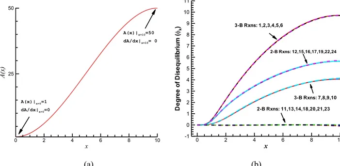
The setup of interest is one that was also considered in [12]. It involves supersonic relaxation of combustion products within a diverging nozzle with an area profile as shown in Figure 1a. The nozzle has an exit-to-throat area ratio of 50 and a length 10 times the diameter of the throat section.
(a) (b)
Figure 1. (a) Dimensionless nozzle cross sectional area and (b) Degrees of disequilibrium, , of the 24 reactions in the DKM plotted versus the dimensionless downstream
coordinate along the nozzle axis. x A (x ) 0 2 4 6 8 10 25 50 A(x)|x=0=1 dA/dx|x=0=0 A(x)|x=10=50 dA/dx|x=10= 0 x D e g re e o f D is e q u ili b ri u m (k ) 0 2 4 6 8 10 -1 0 1 2 3 4 5 6 7 8 9 10 11 3-B Rxns: 1,2,3,4,5,6 3-B Rxns: 7,8,9,10 2-B Rxns: 12,15,16,17,19,22,24 2-B Rxns: 11,13,14,18,20,21,23
Table 1. The 24 reactions of the Hydrogen/Oxygen detailed kinetic mechanism considered in [12]
and in the present study, together with the parameters that determine the forward reaction rate constants, the transpose of the matrix of stoichiometric coefficients, and the matrix
representing the main governing constraints as identified in [12].
Species: j = 1 2 3 4 5 6 7 8 O O2 H H2 OH H2O HO2 H2O2 Reaction 1 O+O+M=O2+M 1.20E+17 -1 0 -2 1 0 0 0 0 0 0 2 O+H+M=OH+M 5.00E+17 -1 0 -1 0 -1 0 1 0 0 0 3 H+H+M=H2+M 1.00E+18 -1 0 0 0 -2 1 0 0 0 0 4 H+H+H2=H2+H2 9.00E+16 -0.6 0 0 0 -2 1 0 0 0 0 5 H+H+H2O=H2+H2O 6.00E+19 -1.3 0 0 0 -2 1 0 0 0 0
6 H+OH+M=H2O+M 2.20E+22 -2 0 0 0 -1 0 -1 1 0 0
7 H+O2+M=HO2+M 2.80E+18 -0.9 0 0 -1 -1 0 0 0 1 0
8 H+O2+O2=HO2+O2 2.08E+19 -1.2 0 0 -1 -1 0 0 0 1 0
9 H+O2+H2O=HO2+H2O 1.13E+19 -0.8 0 0 -1 -1 0 0 0 1 0
10 OH+OH+M=H2O2+M 7.40E+13 -0.4 0 0 0 0 0 -2 0 0 1
11 O+H2=H+OH 3.87E+04 2.7 6260 -1 0 1 -1 1 0 0 0
12 O+HO2=OH+O2 2.00E+13 0 0 -1 1 0 0 1 0 -1 0
13 O+H2O2=OH+HO2 9.63E+06 2 4000 -1 0 0 0 1 0 1 -1
14 H+O2=O+OH 2.65E+16 -0.7 17041 1 -1 -1 0 1 0 0 0
15 H+HO2=O+H2O 3.97E+12 0 671 1 0 -1 0 0 1 -1 0
16 H+HO2=O2+H2 4.48E+13 0 1068 0 1 -1 1 0 0 -1 0
17 H+HO2=OH+OH 8.40E+13 0 635 0 0 -1 0 2 0 -1 0
18 H+H2O2=HO2+H2 1.21E+07 2 5200 0 0 -1 1 0 0 1 -1
19 H+H2O2=OH+H2O 1.00E+13 0 3600 0 0 -1 0 1 1 0 -1
20 OH+H2=H+H2O 2.16E+08 1.5 3430 0 0 1 -1 -1 1 0 0
21 OH+OH=O+H2O 3.57E+04 2.4 -2110 1 0 0 0 -2 1 0 0
22 OH+HO2=O2+H2O 1.45E+13 0 -500 0 1 0 0 -1 1 -1 0
23 OH+H2O2=HO2+H2O 2.00E+12 0 427 0 0 0 0 -1 1 1 -1
24 HO2+HO2=O2+H2O2 1.30E+11 0 -1630 0 1 0 0 0 0 -2 1
i Some notable constraints
EH Total number of hydrogen nuclei 0 0 1 2 1 2 1 2 EO Total number of oxygen nuclei 1 2 0 0 1 1 2 2 M Total number of moles 1 1 1 1 1 1 1 1 FV Total free valence 2 0 1 0 1 0 1 0 FO Total free oxygen 1 0 0 0 1 1 0 0
The dimensionless coordinate denotes the ratio of centerline downstream distance from throat to throat diameter. The dimensionless area denotes the ratio of nozzle cross sectional area to throat area. At the throat the inlet flow conditions are sonic based on frozen Mach number. Temperature and pressure at the throat are 3000 K and 25 atm, respectively, and the mixture is assumed to be at chemical equilibrium. The residence time within the nozzle is 3.7 ms.
Table 1 shows the 24 reactions of the Hydrogen/Oxygen DKM assumed here and in [12]. It also shows the parameters that determine the forward reaction rate constants
(1)
in mol-cm-s-K units with the forward activation energy in cal/mol. The backward reaction rate constants are determined from the principle of detailed balance,
(2)
(3)
is the reaction equilibrium constant (based on concentration). Also, , , where and are the forward and reverse stoichiometric coefficients of the -th reaction, respectively, and is its Gibbs free energy at standard pressure and temperature . In the present paper, we use the notation of [4], which differs only slightly from that of [12].
The degree of disequilibrium of reaction , is defined as follows
(4)
where and are the forward and reverse reaction rates, defined as
and
(5)
where is the number of species in the kinetic model. For convenience of the discussion below, we denote the degree of disequilibrium of a reaction also by or simply DoD. Figure 1b shows for all 24 reactions how the respective DoDs evolve along the axis of the diverging nozzle as the temperature drops rapidly due to the supersonic expansion.
It is worth noticing that the DoD of reaction is related to its de-Donder affinity, as follows (6) where is the chemical potential of species in the mixture. The mathematical interpretation of Eq. (6) is that the DoD of a reaction is a linear combination of the rows of the stoichiometric matrix, with as the coefficients of the linear combination. This means that if some columns of the stoichiometric matrix are linearly dependent, then so are the corresponding DoDs. Said differently, if there exists a set of coefficients such that for every , then, by Eq. (6), we also have .
Finally, the non-equilibrium law of mass action for reaction can be shown to relate to its DoD as follows (combine Eqs. 110 and 112 of [4])
(7)
At the throat, all reactions are at equilibrium, i.e., for every . Downstream, the quick change in nozzle area causes a decrease in temperature, rapid enough to prevent the slow reactions from remaining near equilibrium and, hence, their DoDs build up as the fluid elements move downstream.
3. Preliminary observations about DoDs in the underlying DKM
The main observation in [12] is that the plots in Fig.1b show clearly that for the given nozzle geometry and flow conditions every reaction in the group 11-13-14-18-20-21-23, that we refer to as
"group 0", maintains an approximately vanishing DoD throughout the nozzle. This means that these reactions are able to equilibrate quickly, in the sense that their DoDs remain very close to zero all along the nozzle. Therefore, on the time scale of interest for the given nozzle geometry and flow conditions, these reactions are not slowed down by any of the kinetic bottlenecks which control the spontaneous relaxation towards chemical equilibrium. In other words, the constraints associated with the controlling bottlenecks are not directly affected by the advancement of any of these reactions.
Denoting constraint functionals of the composition vector as follows
(8)
and recalling that , the rates of change of the constraint functionals under the DKM are given by
(9)
where is the number of reactions in the DKM and
(10)
represents the contribution of the net rate of reaction to the rate of change of constraint functional . In order for constraint functional to be unaffected directly by the net rate of reaction it is necessary and sufficient that be zero, or at least very small. Geometrically, this means that the -th row of -the constraint matrix is orthogonal to the -th column of the stoichiometric matrix . This orthogonality condition is automatically satisfied for the two rows and of the constraint matrix that represent the number of atomic nuclei of hydrogen and oxygen, respectively. This is because and are zero for every reaction in the DKM, as required by the physical constraint of conservation of atomic nuclei in chemical reactions. Similarly, the fact that reactions in "group 0" have vanishing DoDs requires that the rows of the constraint matrix corresponding to every constraint (bottleneck) which effectively controls the dynamics, must be orthogonal to the columns 11-13-14-18-20-21-23 of the stoichiometric matrix .
The above observation is shown in [12] to provide an important clue for the selection of constraints. There, according to the traditional RCCE approach [1-8], constraints are assumed to be linear combinations of a set of known physically meaningful constraints, such as EH (total number of hydrogen nuclei), EO (total number of oxygen nuclei), M (total number of moles), FV (free valence), FO (free oxygen), and a few others. The fact that a constraint must not be affected by the (two-body) reactions 11-13-14-18-20-21-23 provides a strong condition that when integrated with well-educated chemical kinetic reasoning and analysis of the DKM, can be exploited, as in [12], to come up with a good semi-empirical choice of a set of governing RCCE constraints. Indeed, very good approximation of the full H/O DKM results have been obtained in [12] using RCCE with a set of only three constraints (M, FO, FV) in addition to the two required by conservation of atomic elements (EH, EO).
Despite its remarkable performance, however, the analysis presented in [12] to construct constraints cannot be claimed to be "systematic", as the authors made note of some contradictory information
implied by one or few reactions in formulating the constraints. It is the aim of the next section to devise a mathematical approach that fully rationalizes the constraint selection for this problem.
4. Additional observations about DoDs in the underlying DKM
The main observation that we put forward in this section and on which we elaborate in the rest of the present paper, is that, in addition to the "equilibrated reactions" (those with approximately zero DoDs, i.e., zero affinity), the non-zero DoDs in Figure 1b also carry additional information that is important for constraint selection. Obviously, they partition the reactions with non-zero DoDs into three other groups of reactions that to a high degree of approximation share at every downstream position the same value of DoD. Indeed, as already shown in [12,27] and discussed in the previous section, important indications can be extracted from the DoD=0 group (the group of equilibrated reactions). However, the fact that when pulled out of equilibrium at a particular rate the reactions turn out to bin themselves into one of a small number of groups characterized by levels of DoD shared exactly or approximately by all reactions in the group, provides additional indications that allow to fully pin down the governing constraints.
While the DoD=0 "group 0" identifies several possible constraints, each of the other groups, which appears to be characterized by a common relaxation time, furnishes (by analogous inspection) tighter indications useful to identify the rate-controlling bottlenecks of the overall kinetic mechanism that are effective at such time scale. To be more specific, the fact that Figure 1b shows for each downstream position three clearly grouped nonzero levels of DoD, is an indication that there are only two bottlenecks, i.e., the controlling constraints are only two: one responsible for a profile of DoD along the nozzle that is common to all reactions in "group A": 7-8-9-10 and we may denote by (this turns out to be the M constraint), the other responsible for a DoD profile that is common to all reactions in "group B": 12-15-16-17-19-22-24 and we denote by (this turns out to be identifiable with the FO-FV constraint). Reactions 1-2-3-4-5-6 instead form a third group that we call "group A+B" because it exhibits a DoD profile that is the sum of the preceding two, i.e., . This clearly means that reactions in group A+B are effectively slowed down by both bottlenecks A and B.
The above observation is enough to identify the two corresponding constraints A and B. Indeed, 1) reactions in Group 0 have no direct effect on either of the rates and ;
2) reactions in Group A have no direct effect on the rate ; 3) reactions in Group B have no direct effect on the rate .
5. New constraint selection methodology
Based on the observations in the previous section, we can conclude that:
1) the row of the constraint matrix is orthogonal to the subset of columns of the stoichiometric matrix with = 11-13-14-18-20-21-23 and 12-15-16-17-19-22-24, i.e., for all the reactions in Groups 0 and B,
or equivalently (11)
where denotes the column vector with components and the transpose of matrix . 2) the row of the constraint matrix is orthogonal to the subset of columns of the stoichiometric matrix with = 11-13-14-18-20-21-23 and 7-8-9-10, i.e., for all the reactions in Groups 0 and A,
or equivalently (12)
where is the column vector with components and the transpose of matrix .
3) It is useful to remind that the row and the row of the constraint matrix are orthogonal to all the columns of the stoichiometric matrix for from 1 to , i.e., for all the reactions in the DKM,
or equivalently and (13) where we denote by and the column vectors with components and , respectively. As a consequence of Eqs. (13), once we have found vectors and that satisfy Eqs. (11) and (12), respectively, than we can substitute the linearly independent set of constraints , , ,
with any other linearly independent set of vectors in their linear span.
From linear algebra, equation means that vector is in the null space (kernel) of the matrix and vector in the null space (kernel) of the matrix . If we compute we find that it is three dimensional (to compute the kernel, we use the MatLab function kA=null(A,'r') which applies the Gauss elimination algorithm to compute the basis of the kernel of matrix A, returned as the columns of matrix kA). In fact, it is the linear span of three linearly independent constraints: , , and . However, we can easily identify the component of
orthogonal to the two dimensional linear span of constraints and , by computing instead the null space of the matrix
(14)
obtained by appending to matrix the column vectors representing the elemental constraints and then taking the transpose. Table 2 shows the transpose of matrix and the single vector which constitutes the basis of the one-dimensional . As noted in Table 2, is a linear combination of constraints (EH, EO, M).
Table 2. The transpose of matrices and whose kernels uniquely identify the two constraints effectively controlling the kinetics under the nozzle geometry and boundary conditions that generate the full DKM profiles of DoD shown in Figure 1b.
Matrix 11 13 14 18 20 21 23 12 15 16 17 19 22 24 EH EO -1 -1 1 0 0 1 0 -1 1 0 0 0 0 0 1 0 -5/4 1 0 0 -1 0 0 0 0 1 0 1 0 0 1 1 2 0 -1/2 1 1 0 -1 -1 1 0 0 0 -1 -1 -1 -1 0 0 0 1 -5/4 1 -1 0 0 1 -1 0 0 0 0 1 0 0 0 0 0 2 -1/2 1 1 1 1 0 -1 -2 -1 1 0 0 2 1 -1 0 1 1 -1/2 1 0 0 0 0 1 1 1 0 1 0 0 1 1 0 1 2 1/4 1 0 1 0 1 0 0 1 -1 -1 -1 -1 0 -1 -2 2 1 1/4 1 0 -1 0 -1 0 0 -1 0 0 0 0 -1 0 1 2 2 1 1 Matrix 11 13 14 18 20 21 23 7 8 9 10 EH EO -1 -1 1 0 0 1 0 0 0 0 0 1 0 -19/4 -1 0 0 -1 0 0 0 0 -1 -1 -1 0 2 0 5/2 0 1 0 -1 -1 1 0 0 -1 -1 -1 0 0 1 -27/4 -1 -1 0 0 1 -1 0 0 0 0 0 0 0 2 -3/2 0 1 1 1 0 -1 -2 -1 0 0 0 -2 1 1 1/2 0 0 0 0 0 1 1 1 0 0 0 0 1 2 23/4 1 0 1 0 1 0 0 1 1 1 1 0 2 1 -17/4 -1 0 -1 0 -1 0 0 -1 0 0 0 1 2 2 1 0
Similarly, is the linear span of , , and . So, to identify the component of orthogonal to the two dimensional linear span of constraints and , we compute the null space of the matrix
(15)
obtained by appending to matrix the column vectors representing the elemental constraints and then taking the transpose. Table 2 shows also the transpose of matrix and the single vector which constitutes the basis of the one-dimensional . As noted in Table 2, is a linear combination of constraints (EH, EO, FO-FV).
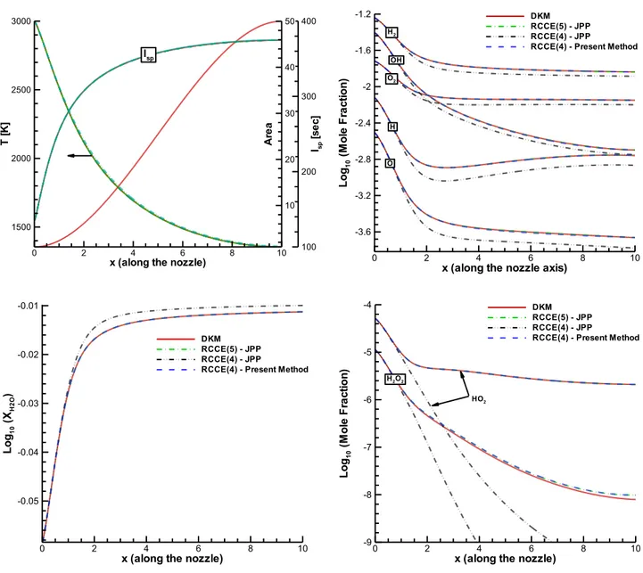
Figure 2. Plots of temperature , specific impulse , and mole fractions of all species versus dimensionless downstream axial distance resulting from RCCE simulations compared with the corresponding data from the underlying DKM simulation, for the same nozzle dimensionless area
and sonic throat inlet conditions as in [12]. The constraints used in the different RCCE
simulations are: the two sets of constraints obtained in [12], namely, the 5-constraints set
RCCE(5)-JPP = (EH, EO, M, FO, FV) and the 4-constraints set RCCE(4)-JPP = (EH, EO, H+H2,
O+OH+H2O); and the 4-constraints set RCCE(4)-PresentMethod = (EH, EO, M, FO-FV) resulting
from the selection methodology presented here. x (along the nozzle)
T [K ] Isp [s e c] A re a 0 2 4 6 8 10 1500 2000 2500 3000 100 200 300 400 10 20 30 40 50 Isp
x (along the nozzle axis)
L o g10 (M o le F ra ct io n ) 0 2 4 6 8 10 -3.6 -3.2 -2.8 -2.4 -2 -1.6 -1.2 DKM RCCE(5) - JPP RCCE(4) - JPP
RCCE(4) - Present Method
O H2
O2 OH
H
x (along the nozzle)
L o g10 (X H 2 O ) 0 2 4 6 8 10 -0.05 -0.04 -0.03 -0.02 -0.01 DKM RCCE(5) - JPP RCCE(4) - JPP
RCCE(4) - Present Method
x (along the nozzle)
L o g10 (M o le F ra ct io n ) 0 2 4 6 8 10 -9 -8 -7 -6 -5 -4 DKM RCCE(5) - JPP RCCE(4) - JPP
RCCE(4) - Present Method
H2O2
Finally, therefore, the main result of the new algorithm is that it identifies automatically the set of four constraints (EH, EO, M, FO-FV) as the one effectively governing the dynamics under the given geometry and boundary conditions. Importantly, it does so with no need for any additional physical insight, other than the inspection of the grouping of reactions that in Figure 1b is quite evident.
To validate the method so far, Figure 2 shows the results of an RCCE simulation using the 4-constraints set (EH, EO, M, FO-FV) compared with the results of the DKM simulation as well as the RCCE simulations based on the sets of constraints obtained in [12], namely, the 5-constraints set (EH, EO, M, FO, FV) and the 4-constraints set (EH, EO, H+H2, O+OH+H2O). The specific impulse is defined as the thrust force per unit mass flow rate of the propellant. Under the assumed isentropic expansion to back pressure throughout the nozzle, it is equal to the flow velocity at the nozzle exit plane, . In rocketry it is common to divide the specific impulse by the gravitational acceleration, , to make it independent of the system of units. Therefore,
, which has units of time.
The results are very encouraging and so in a forthcoming separate paper we provide an automatic algorithm also for grouping the reactions based on the analysis of DoD results from the DKM simulation. Indeed, it is possible to further systematize our new methodology for RCCE constraint selection for full automation also of the reaction grouping step, which in the present paper we achieve easily by inspection of Figure 1b, but in more general cases can be much less immediate, especially when more than 2 bottlenecks are in effect. Indeed, with two bottlenecks we have seen that the reactions essentially assemble into 4 basic groups (0, A, B, A+B) but in principle also other possible combinations like A+2B and so on are possible. With three bottlenecks, reactions can form at least 8 basic groups (0, A, B, C, A+B, A+C, B+C, A+B+C) but again also higher integer and even fractional linear combinations are in principle possible. With four bottlenecks, the basic groups are 16 (0, A, B, C, D, A+B, A+C, A+D, B+C, B+D, C+D, A+B+C, A+B+D, A+C+D, B+C+D, A+B+C+D) plus other combinations. It is clear that the identification by simple inspection becomes very difficult, if not impossible, as the number of bottlenecks increases beyond three. However, we show elsewhere that this apparent complexity can also be mathematically rationalized for full automation of constraint selection.
6. Conclusions
The Rate-Controlled Constrained-Equilibrium (RCCE) method provides a strong thermodynamically consistent general reduction framework to model, with good degrees of approximation, complex chemical kinetics in applications involving shifting equilibrium, frozen equilibrium, as well as highly non-equilibrium kinetic problems, by solving a significantly lower number of differential equations than required by a full Detailed Kinetic Model (DKM). To provide accurate approximations, the method requires that we identify the bottleneck kinetic mechanisms responsible for slowing down the relaxation of the state of the system towards local chemical equilibrium. More precisely, the method requires that such bottleneck mechanisms be characterized by means of a set of representative constraints. So far, a weakness of the method has been the absence of a systematic algorithm that would allow a fully automatable identification of the best constraints for a given range of conditions and required level of approximation.
In this paper we have provided the first of two steps towards a systematic algorithm that allows a fully automatable identification of the best constraints required to implement for a given range of conditions and a level of approximation in the Rate-Controlled Constrained-Equilibrium (RCCE) model reduction method. The algorithm is based on analysing how the degrees of disequilibrium (DoD) of the chemical reactions behave in a full DKM test simulation. The methodology has been exemplified in a quasi one-dimensional study of steady chemical relaxation of the products of the
oxy-combustion of hydrogen expanding through a supersonic nozzle. To provide accurate approximations, the RCCE method requires that we identify the bottleneck kinetic mechanisms that are responsible for slowing down the relaxation of the state of the system towards local chemical equilibrium. More precisely, the bottleneck mechanisms must be characterized by means of a set of representative constraints. When, as for the present example, only two bottleneck kinetic mechanisms are in effect, the DoDs of the chemical reactions assemble into as low as four groups with almost identical behaviour. Once these groups are identified, a kernel analysis of two matrices obtained from the stoichiometric coefficients yields the two constraints that effectively control the dynamics. For illustrative purposes, we have considered an example in which the kinetics are controlled by only two bottlenecks, so that the grouping of reactions can be easily obtained by inspection of how the DoDs of the various reactions behave. In a forthcoming paper, we provide a mathematical algorithm also for the reaction grouping step of the proposed method, thus allowing a fully automated constraint selection also when the number of controlling bottlenecks is large.
References
[1] J.C. Keck and D. Gillespie, Rate-controlled partial-equilibrium method for treating reacting gas mixtures, Combust. Flame, Vol. 17, 237 (1971).
[2] J.C. Keck, Rate-controlled constrained equilibrium method for treating reactions in complex systems, in The Maximum Entropy Formalism, Levine and Tribus, Eds., M.I.T. Press, 1978. [3] G.P. Beretta and J.C. Keck, The constrained-equilibrium approach to nonequilibrium
dynamics. In Proceedings of the ASME Meeting, Anaheim, CA, USA, 7–12 December 1986. In Computer-Aided Engineering of Energy Systems, Second Law Analysis and Modeling; Gaggioli, R.A., Ed.; ASME: New York, NY, USA; ASME Book H0341C-AES, Volume 3, pp. 135–139. Available online: http://www.jameskeckcollectedworks.org/
[4] R. Law, M. Metghalchi, and J.C. Keck, Rate-Controlled Constrained Equilibrium calculations of Ignition Delay Times in Hydrogen-Oxygen Mixtures, XXII Symposium (International) on Combustion, 1988, p. 1705.
[5] J.C. Keck, Rate-controlled constrained-equilibrium theory of chemical reactions in complex systems, Prog. Energy Combust. Sci., Vol. 16, 125-154 (1990).
[6] M. Janbozorgi and H. Metghalchi, Rate-Controlled Constrained-Equilibrium Theory Applied to Expansion of Combustion Products in the Power Stroke of an Internal Combustion Engine, Int. J. of Thermodynamics, Vol. 12, 44-50 (2009).
[7] G.P. Beretta, J.C. Keck, M. Janbozorgi, and H. Metghalchi, The Rate-Controlled Constrained-Equilibrium Approach to Far-From-Local-Constrained-Equilibrium Thermodynamics, Entropy, Vol. 14, 92-130 (2012).
[8] G. Nicolas, M. Janbozorgi, and H. Metghalchi, Constrained-Equilibrium Modeling of Methane Oxidation in Air, ASME Journal of Energy Resources Technology, Vol. 136, 032205 (2014).
[9] V. Hiremath, Z. Ren, and S.B. Pope, A Greedy Algorithm for Species Selection in Dimension Reduction of Combustion Chemistry, Combustion Theory and Modeling, Vol. 14, 619–652 (2010).
[10] V. Hiremath, Z. Ren, and S.B. Pope, Combined Dimension Reduction and Tabulation Strategy Using ISAT-RCCE-GALI for the Efficient Implementation of Combustion Chemistry, Combust. Flame, Vol. 158, 2113–2127 (2011).
[11] S. Rigopolous, and T. Lovas, A LOI-RCCE Methodology for Reducing Chemical Kinetics, with Application to Laminar Premixed Flames, Proceedings of the Combustion Institute, Vol. 32, 569–576 (2009).
[12] M. Janbozorgi and H. Metghalchi, Rate-Controlled Constrained-Equilibrium Modeling of H-O Reacting Nozzle Flow, Journal of Propulsion and Power, Vol. 28, 677-684 (2012).
[14] U. Mass and S.B. Pope, Simplifying chemical kinetics: Intrinsic low-dimensional manifolds in composition space, Combust. Flame, Vol. 88, 239-264 (1992).
[15] S.H. Lam and D.A. Goussis, Understanding complex chemical kinetics with computational singular perturbation, Proceedings of the Combustion Institute, Vol. 22, 931-941 (1988). [16] S.H. Lam, Using CSP to understand complex chemical kinetics, Combustion Science and
Technology, Vol. 89, 375-404 (1993).
[17] V. Mauro, F. Creta, D.A. Goussis, J.C. Lee, and H.N. Najm, An automatic procedure for the simplification of chemical kinetic mechanisms based on CSP, Combust. Flame, Vol. 146, 29-51 (2006).
[18] D.A. Schwer, P. Lu, and W.H. Green, An adaptive chemistry approach to modeling complex kinetics in reacting flows, Combust. Flame, Vol. 133, 451-465 (2003).
[19] I. Banerjee and M.G. Ierapetritou, An adaptive reduction scheme to model reactive flow, Combust. Flame, Vol. 144, 619-633 (2006).
[20] O. Oluwole, B. Bhattacharjee, J.E. Tolsma, P.I. Barton, and W.H. Green, Rigorous valid ranges for optimally reduced kinetic models, Combust. Flame, Vol. 146, 348-365 (2006). [21] M. Rein, The partial-equilibrium approximation in reacting flows, Phys. Fluids A, Vol. 4, 873
(1992), see also the Erratum. ibid., 2930 (1992).
[22] T. Lu and C.K. Law, Linear time reduction of large kinetic mechanisms with directed relation graph: n-Heptane and iso-octane, Combust. Flame, Vol. 144, 24-36 (2006).
[23] Z. Ren, S.B. Pope, A. Vladimirsky, and J.M.J. Guckenheimer, The invariant constrained equilibrium edge preimage curve method for the dimension reduction of chemical kinetics, J. Chem. Phys., Vol. 124, 114111 (2006).
[24] A.N. Gorban and I.V. Karlin, Method of invariant manifold for chemical kinetics, Chemical Engineering Science, Vol. 58, 4751 (2003).
[25] T. Lovas, Automatic generation of skeletal mechanisms for ignition combustion based on level of importance analysis, Combust. Flame, Vol. 156, 1348–1358 (2009).
[26] M. Kooshkbaghi, C.E. Frouzakis, K. Boulouchos, and I.V. Karlin, Entropy production analysis for mechanism reduction, Combust. Flame, Vol. 161, 1507 (2014).
[27] V. Yousefian, A Rate-Controlled Constrained-Equilibrium Thermochemistry Algorithm for Complex Reacting Systems, Combust. Flame, Vol. 115, 66–80 (1998).
![Table 1. The 24 reactions of the Hydrogen/Oxygen detailed kinetic mechanism considered in [12]](https://thumb-eu.123doks.com/thumbv2/123dokorg/5507725.63607/4.892.129.760.163.767/table-reactions-hydrogen-oxygen-detailed-kinetic-mechanism-considered.webp)