0D-1D thermo-fluid dynamic modelling of cylinder scavenging process in a four stroke IC engine

Industrial Engineering

Energy Engineering, Power Production

0D-1D THERMO-FLUID DYNAMIC MODELLING

OF CYLINDER SCAVENGING PROCESS

IN A FOUR STROKE IC ENGINE

Tesi di Laurea di :

Christian Leoni Matr. 892162 Gianmarco Latella Matr. 892266

Relatore: Prof. Angelo Onorati Correlatore: Dott. Andrea Massimo Marinoni

Nowadays environmental topics, such as air pollution and global warming, are increasingly popular on the scientific debate. Focusing on the automotive sector, progressively stricter regulations have been applied on new designed cars, since internal combustion engines, together with tyres and brakes, are one of the major sources of local pollutants.

The aim of this thesis is to improve the performance of Gasdyn, a 1D en-gine simulation tool developed by the Energy Departement of Politecnico di Milano, in the prediction of pollutants emissions. In particular, we will con-centrate our attention on the evaluation of unburned hydrocarbons emissions from SI engines, by means of a new model for cylinder scavenging.

Engine Gasdynamics Fundamental Equations

Gasdynamics in internal combustion engines is characterized by three dimen-sionality, unsteadiness and turbulence; thus, in order to completely represent the flowfield inside an IC engine, a 3D mathematical model should be ap-plied. However, this kind of model involves the system of 3D Navier Stokes equations, which cannot be solved analytically but just numerically, with an enormous computational effort.

with a 3D approach. This latter is adopted just for single pieces of equip-ment, while a 1D model has to be considered for the whole architecture, with the following fundamental assumptions:

• unsteady flow;

• one-dimensional flow: the longitudinal dimension of the duct-systems is significantly greater than the transversal one;

• compressible fluid: perfect gas model, with constant specific heats, or mixture of ideal gases, with specific heats depending both on temper-ature and composition;

• friction and heat transfer only at the gas-wall interface; • non-adiabatic and non-isentropic flow;

• variable cross-section with assigned law.

In order to describe the fluid dynamics of flows inside pipes and cylinders, four conservation equations are applied:

• Mass Conservation: ∂ρ ∂t + ∂(ρu) ∂x + ρu F dF dx = 0 • Momentum Conservation: ∂u ∂t + u ∂u ∂x + 1 ρ ∂p ∂x + G = 0

∂(ρe0) ∂t + ∂(ρuh0) ∂x + ρuh0 F dF dx − ρ ˙q − ∆HreactF dx = 0 • Transport of Species: ∂ ∂t(ρF Yj) + ∂ ∂x(ρuF Yj) + ρF ˙Yj = 0

These equations are difficult to manage as they are; therefore, a matrix form is derived from them:

∂ ∂t ~ W (x, t) + ∂ ∂x ~ F ( ~W ) + ~B( ~W ) + ~C( ~W ) = 0

where: ~W (x, t) is the conserved variables vector, ~F ( ~W ) is the fluxes vector, ~

B( ~W ) and ~C( ~W ) are the vectors of source terms.

~ W =         ρF ρuF ρe0F ρ~Y F         ~ F =         ρuF (ρu2_{+ p)F} ρuh0F ρu~Y F         ~ B =         0 −pdF dx 0 0         ~ C =         0 ρGF −(ρ ˙q + ∆Hreact)F ρ ˙Y F        

As far as it concerns pollutants emission, SI engines mainly emits Nitrogen Oxides (NOx), Carbon Monoxide (CO) and Unburned Hydrocarbons (HC).

Focusing on the last item, since it is the main target of the former analysis, the most important sources of HC are:

• crevices: fuel mass stored inside cylinder crevices cannot be reached by the flame front, thus unburned hydrocarbons are emitted in the exhaust;

• oil film: the fluid layer on the cylinder wall can absorb fuel hydro-carbons when the partial pressure is high, then release them during expansion stroke;

• quenching: when the flame front approaches cylinder walls it can be extinguished, if temperature is too low. This phenomenon is more likely at cold start and it results in unburned fuel emission;

• scavenging: during valve overlap period, part of the fresh mixture could directly flow from the intake through the exhaust port, so that part of the cylinder unburned fuel is emitted.

The purpose of this work is to enhance the predictivity of HC emissions due to cylinder scavenging. In the overlap period, three main gas exchange phe-nomena occur inside the cylinder: short circuit of unburned mixture directly through the exhaust port; mixing between unburned and burned mixtures; inlet backf low.

The model implemented in the original code describes the cylinder as a sin-gle zone volume, in which perfect mixing happens; thus, the residuals from

regions. This model is well predictive of CO and NOx emissions, as well as

HC from crevices and oil film. However, it is not capable to properly predict the HC emitted during the overlap period.

The proposed scavenging model considers four zones, as shown in figure 1: 1. cylinder unburned zone;

2. cylinder burned zone; 3. inlet duct;

4. exhaust duct;

1. Intake → U nburned 2. Burned → Exhaust

3. U nburned → Burned : M ixing

4. U nburned → Exhaust : Short Circuit                  Primary Fluxes 5. Intake → Burned 6. U nburned → Exhaust    Secondary Fluxes

This complex framework can be visualized in the picture below (3.11).

• Primary fluxes of fresh mixture are portrayed in blue; • The only primary flux of burned gases is in orange; • The two secondary fluxes are represented in black; • The fuel injected is in green.

Short circuit and mixing fluxes are evaluated by means of two calibration parameters, KSHC and KM IX, which depend on the turbulence intensity

inside the cylinder and vary from 0 to 1. Specifically, these mass flow rates are expressed as:

dmSHC = KSHC· min [dmIN; dmOU T]

dmM IX = KM IX · (dmIN − dmSHC)

Sensitivity analysis results

First of all, the theoretical model validation is performed by means of a sensitivity analysis on two samples: a single cylinder, 2 valves spark ignition engine and a four cylinders, 16 valves spark ignition engine. The validation is done by comparing scavenging model results to original ones, focusing on two quantities: the average emitted mass of HC during a cycle [g], plotted for each rotational speed, and the HC instantaneous outgoing flux at a fixed regime [g/s].

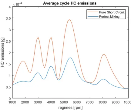
• perfect mixing, i.e. KM IX = 1, KSHC = 0;

• pure short circuit, i.e. KM IX = 0, KSHC = 1;

• turbulence intensity dependence, KM IX = KSHC = f (u0)

Perfect mixing

In case of perfect mixing, the model behaves as the original code, as charts 3 and 4 show. This situation is absolutely reasonable, since a change in the zones number should not imply a significant difference in the final results.

Pure short circuit

When pure short circuit is investigated, an increase of both cycle average and instantaneous HC emissions is expected, since a portion of the fresh charge by-passes the cylinder without any mixing with the burned volume. This situation is unwanted because it is the worse in terms of HC emissions and brake specific fuel consumption (BSFC), thus engine efficiency.

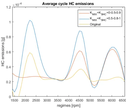
Two limiting cases have been considered so far; now, the general situation is presented. According to [11], we can identify a correlation between cylinder turbulence intensity u’ and the calibration coefficients, i.e. function f1(u0) in

table 1. However, this correlation does not capture the HC emission when the turbulence is too low. Therefore, f2(u0) is proposed as alternative law.

Interval f1(u0) f2(u0)

0 < u0 < 3 KM IX = KSHC = 0 KM IX = KSHC = 0.5

3 < u0 < 4 KM IX = KSHC = 0.5 KM IX = KSHC = 0.8

u0 > 4 KM IX = KSHC = 0.9 KM IX = KSHC = 1

Table 1: Calibration coefficients as function of the turbulence intensity The single cylinder sample is characterized by a too low turbulence intensity at any engine speed, so that the performance of the proposed correlations for the scavenging model have to be analyzed on a more complex architecture: the four cylinders Alfa Romeo SI engine. The obtained results are reported in charts 7 and 8.

As expected, f1(u0) considers neither mixing nor short circuit occurring in

case of low turbulence intensity (KM IX = KSHC = 0 if u0 < 3), resulting in

a flat trend at low regimes. The main outcome of the sensitivity analysis is that f2(u0) seems to behave better along the whole rotational speed range.

Moreover, through-flow magnitude over mixing increases with the engine regime, since the difference between the scavenging model profiles and the original one enlarges with rotational speed.

An experimental validation of the scavenging model is required to confirm the results of the sensitivity analysis.

The sample exploited for this purpose is the Lamborghini V10, 5.0 litres, 40 valves, spark ignition engine. This architecture is more complex than the two considered so far: a more accurate investigation of the influence of turbulence intensity on the calibration coefficients can be realized.

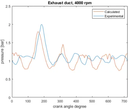
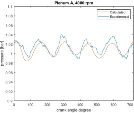
First of all, an engine performance validation is carried out, by comparing the Gasdyn calculated values to the experimental ones. Pressure is analyzed in many engine points: in intake and exhaust ducts, inside the cylinder, in aspiration manifold plenums. Moreover, volumetric efficiency, brake torque and brake power are considered for both the original and the scavenging model, without showing significant differences.

Once the engine sample is validated, the analysis on the HC emissions is performed. The average HC concentration in the exhaust duct is considered as reference quantity.

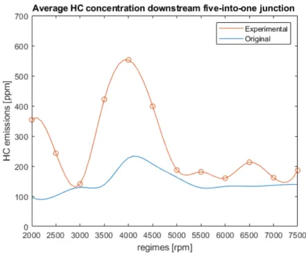
First of all, the original model results are compared to the experimental ones: from chart 17 it is clear that the old code is not satisfactory in the prediction of HC emitted.

Therefore, the scavenging model is applied to the same sample, providing the results portrayed in chart 18. Both the correlations are good to predict the peak of HC at 4000 rpm. However, f2(u0) is better because of the following

reasons:

1. higher HC peak emissions at 4000 rpm, closer to the experimental trend;

Extended abstract 2 Summary 25 Sommario 26 1 Gas Dynamics 29 1.1 Conservation Equations . . . 29 1.1.1 Mass conservation . . . 31 1.1.2 Momentum conservation . . . 31 1.1.3 Energy conservation . . . 33 1.1.4 Strong Conservative form . . . 34 1.1.5 Transport of chemical spiecies . . . 38 2 Spark Ignition Engine Pollutant Emissions 41 2.1 Combustion model . . . 44 2.1.1 Two-zone model . . . 44 2.1.2 Multizone model . . . 45 2.2 Carbon Monoxide . . . 48 2.2.1 Formation . . . 48 2.2.2 Prediction Model . . . 49

2.3 Nitrogen oxides . . . 52 2.3.1 Formation . . . 52 2.3.2 Prediction Model . . . 55 2.4 Unburned hydrocarbons . . . 57 2.4.1 Formation . . . 57 2.4.2 Prediction Model . . . 61 3 Scavenging model 65 3.1 Introduction . . . 65 3.2 Cylinder scavenging process . . . 66 3.2.1 Original cylinder model . . . 68 3.2.2 Scavenging submodels . . . 69 3.3 Scavenging model . . . 78 3.3.1 Fundamental assumptions . . . 78 3.3.2 Mass fluxes . . . 83 3.3.3 Mass balances . . . 89 3.4 Turbulence . . . 92 3.4.1 Turbulence in SI engines . . . 92 3.4.2 K-k model for turbulence intensity . . . 96 4 Theoretical model validation 101 4.1 Single cylinder engine . . . 101 4.1.1 KM IX and KSHC sensitivity analysis . . . 102

4.1.2 Valve overlap period: sensitivity analysis . . . 109 4.1.3 NOx and CO emissions . . . 112

4.2 Alfa Romeo 4 cylinders engine . . . 114 5 Experimental model validation 119

5.2 Engine performance validation . . . 122 5.3 Pollutant emissions . . . 131 5.3.1 NOx and CO emissions . . . 131

5.3.2 Unburned HC emissions . . . 134

The aim of this thesis is to investigate the cylinder scavenging process in internal combustion SI engines, in order to predict unburned HC emissions. The original model implemented in Gasdyn, a software developed by the En-ergy Department of Politecnico di Milano, considers a single zone geometry for the cylinder, where perfect mixing of fresh charge with residuals happens. The new implemented model for scavenging, instead, is based on a four zones geometry. By tracking the mass fluxes among these regions, an improvement in the gas exchange process description is achieved: both mixing and short circuit phenomena are captured; furthermore, their magnitude is investigated as function of the cylinder turbulence intensity.

The results of the sensitivity analysis, performed on two simple engine ar-chitectures, as well as the experimental model validation, carried out on the Lamborghini V10 engine, allow to properly tune the calibration coefficients for mixing and short circuit.

The scavenging model improves the predictivity of HC emissions with re-spect to the original one, by keeping the same reliability in the analysis of performance parameters, such as volumetric efficiency and brake torque.

Keywords

Lo scopo di questo elaborato di tesi `e l’analisi del processo di lavaggio del cilindro in motori a combustione interna ad accensione comandata, in modo tale da tracciare opportunamente le emissioni di idrocarburi incombusti. Il modello originale implementato in Gasdyn, un software sviluppato dal Dipartimento di Energia del Politecnico di Milano, considera un modello monozona per il cilindro, in cui si verifica un perfetto miscelamento tra car-ica fresca e residui di combustione.

Il nuovo modello di lavaggio `e invece basato su un approccio multizona. L’analisi dei flussi di massa tra le quattro zone garantisce un miglioramento nella descrizione della gasdinamica durante il riempimento del cilindro: in questo modo `e possibile rappresentare sia il miscelamento, sia il corto circuito della carica fresca. Inoltre, l’impatto di questi due fenomeni `e quantificabile mediante un’analisi parametrica in funzione dell’intensit`a di turbolenza. I risultati dell’analisi di sensitivit`a, attuata su due architetture di motore semplici, insieme alla validazione sperimentale del modello, effettuata sul motore Lamborghini V10, consentono di calibrare i coefficienti di miscela-mento e corto circuito.

La predittivit`a delle emissioni di HC nei condotti di scarico migliora medi-ante l’utilizzo del nuovo modello di lavaggio, se paragonata con il modello originale; nonostante ci`o, si mantiene la stessa affidabilit`a nell’analisi delle

performance motoristiche, quali coefficiente di riempimento e coppia.

Parole chiave

lavaggio; idrocarburi incombusti ; miscelamento; corto circuito; intensit`a di turbolenza

Gas Dynamics

1.1

Conservation Equations

Gas dynamics in internal combustion engines is characterized by three di-mensionality, unsteadiness and turbulence; the flow interacts with the wall by means of frictional forces, due to fluid viscosity, and heat transfer. [1] Thus, temperature, pressure and velocity of the gas show relevant gradients inside the ducts.

The mathematical model describing the problem involves the 3D Navier Stokes equations. The analytical solution for such complex systems do not exist, while the numerical one can be achieved by means of a huge com-putational effort. Indeed, the intrinsic unsteadiness of the flow does not allow to solve a Reynolds Averaged Navier Stokes problem (RANS): Large Eddy Simulations (LES) are required to properly deal with the time depend-ing 3D problem. However, this choice is viable only for sdepend-ingle components of the system, such as catalysts, injectors and junctions, where the three-dimensionality of the flow has to be captured.

considered, with the following fundamental assumptions: • unsteady flow;

• one-dimensional flow: the longitudinal dimension of the duct-systems is significantly greater than the transversal one;

• compressible fluid: perfect gas model, with constant specific heats, or mixture of ideal gases, with specific heats depending both on temper-ature and composition;

• friction and heat transfer only at the gas-wall interface; • non-adiabatic and non-isentropic flow;

• variable cross-section with assigned law.

A 1D compressible unsteady flow into an infinitesimal duct element with variable cross-section is considered. Pressure, density and gas velocity are function both of the spatial coordinate x and the time:

The conservation of mass, momentum and energy can be expressed by a system of partial differential equations.

1.1.1

Mass conservation

The variation of mass in the control volume has to be equal to the net flux through the infinitesimal element surface:

(ρ +∂ρ ∂xdx)(u + ∂u ∂xdx)(F + dF dxdx) − ρuF = − ∂ ∂t(ρF dx) By considering just first order infinitesimal terms, we get:

∂ρ ∂t + ∂(ρu) ∂x + ρu F dF dx = 0 (1.1.1)

1.1.2

Momentum conservation

The rate of momentum increase within the control volume equals the summa-tion of the net flux of momentum through the infinitesimal element surface and the resultant of pressure and shear forces acting on the control volume. In order to understand the different contributions to the momentum equa-tion, it can be useful to separately analyze each term.

• Rate of change of momentum:

∂(ρuF dx) ∂t

• Net flux of momentum through the control volume surface: (ρ + ∂ρ ∂xdx)(u + ∂u ∂xdx) 2_{(F +} dF dxdx) − ρF u 2 ₌ ∂(ρF u2) ∂x dx • Pressure forces: pF − (p + ∂p ∂xdx)(F + dF dxdx) + p dF dxdx = −( ∂(pF ) ∂x dx + p dF dxdx) • Friction forces: Ff riction = −f ρu2 2 (πDdx)

f is the friction coefficient between wall and fluid: it can be evaluated as function of Reynolds number and the relative roughness of the duct wall.

Summing up the previous contribution and considering the continuity equa-tion, we get: ∂u ∂t + u ∂u ∂x + 1 ρ ∂p ∂x + G = 0 (1.1.2) where G, the dissipative contribution due to friction, can be expressed as:

G = fu 2 2 u |u| 4 D

1.1.3

Energy conservation

By applying the first law of thermodynamic to the control volume, we can obtain: ˙ Q − ˙W = ∂E0 ∂t + ∂H0 ∂x dx (1.1.3) where:

• ˙Q is the rate of heat transferred from gas to the duct walls and vicev-ersa. It can be expressed as follows:

˙

Q = ˙qρF dx + ∆HreactF dx

where ˙q is the heat transfer per unit mass per unit time, while ∆Hreactis

the heat released (per unit volume per unit time) by chemical reactions in gas phase.

• ˙W is the work done on or by the system, that is zero for a gas flowing in a duct of the engine.

• ∂E0

∂t is the variation of stagnation internal energy, equal to:

∂E0

∂t = ∂

∂t(e0ρF dx)

where the specific stagnation internal energy can be expressed as: e0 = e +

U2

2 = cvT + U2

• ∂H0

∂x is the net efflux of stagnation enthalpy through the control surface:

∂H0

∂x = ∂

∂x(h0ρF u)

where the specific stagnation enthalpy can be expressed as: h0 = e0 +

p ρ

By summing up all the previous elements, assuming no work, we obtain the following form of the Energy Conservation equation:

∂(ρe0) ∂t + ∂(ρuh0) ∂x + ρuh0 F dF dx − ρ ˙q − ∆HreactF dx = 0 (1.1.4)

1.1.4

Strong Conservative form

In order to solve the hyperbolic system of partial derivative non linear equa-tions, the strong conservative formulation is adopted, since it better accom-plishes with the numerical methods requirements. This consideration implies to switch from momentum conservation equation to impulse conservation equation, since this latter quantity is conserved in case of shock waves, which are frequent phenomena occuring in engine ducts.

                   ∂ ∂t(ρF ) + ∂ ∂x(ρuF ) = 0 Continuity ∂ ∂t(ρuF ) + ∂ ∂x((p + ρu 2_{)F ) − p}dF dx + ρGF = 0 Impulse ∂ ∂

The second equation highlights the quantity p + ρu2, which is the impulse. On the basis of the strong conservative form, it is convenient to express the hyperbolic problem in matricial form, in order to apply shock-capturing numerical methods.

Four vectors are introduced, each of them containing terms of continuity, impulse and energy equation.

• Vector of conserved variables

~ W =      ρF ρuF ρe0F     

It contains three groups of independent gasdynamic variables that vary with x and t. • Vector of fluxes ~ F =      ρuF (ρu2+ p)F ρuh0F     

• Vectors of source terms

~ B =      0 −pdF dx 0      ~ C =      0 ρGF −(ρ ˙q + ∆Hreact)F     

The first vector ~B does not contain any dissipative term, since −pdF_dx is related to the variable geometry of pipes. Vector ~C, instead, accounts for dissipative contribution due to friction and heat transfer: these phenomena prevent the flow from being isentropic.

Thus, the hyperbolic system can be written in a more compact form: ∂ ∂t ~ W (x, t) + ∂ ∂x ~ F ( ~W ) + ~B( ~W ) + ~C( ~W ) = 0 (1.1.5)

The current problem involves three equations in four unknowns (ρ, u, e, p). Therefore, a fourth equation is introduced.

A first model implemented in the code is the perfect gas one, with the fluid behaviour described by the ideal gas law:

pV = N RT (1.1.6)

where R=8.314 _mol·KJ is the universal gas constant.

Furthermore, the constant volume specific heat is constant, depending just on the degrees of freedom of the fluid molecules.

In this way, the specific stagnation internal energy and enthalpy may be expressed as: e0 = cvT + u2 2 = p ρ(k − 1) + u2 2 (1.1.7) h0 = cpT + u2 2 = kp ρ(k − 1) + u2 2 (1.1.8)

However, a more general model is also implemented in the code: the fluid is considered as an ideal mixture of ideal gases and each of the species follows the ideal gas law:

pj ρj = RjT = R M Mj T (1.1.9)

For the whole mixture, the governing equation becomes: p = ρRT

PNspecies

j=1 XjM Mj

(1.1.10)

where Xj is the molare fraction of the j-th species, and M Mj its molar mass;

the denominator of the previous equation, instead, represents the molar mass of the whole mixture, calculated as the weigthed average of its components. The molar enthalpy and internal energy of the j-th specie of the mixture can be expressed by means of the following polynomial relationships, in which the coefficients αM j for each chemical species have been determined on the

basis of the JANAF and NASA data.

hj(T ) = R · (α1jT + α2j 2 T 2 + α3j 3 T 3 +α4j 4 T 4 +α5j 5 T 5 + α6j) (1.1.11) ej(T ) = hj(T ) − RT (1.1.12)

The model implemented in the code is then simplified, by considering the specific internal energy as a quadratic function of temperature:

ej(T ) = α1jT + α2jT2 (1.1.13)

the fifth order polynomial curve in a prefixed temperature range. As for the whole mixture, the global coefficients α1, α2 can be obtained as weighted

average on the different species:

α1 = Nspecies X j=1 α1jXj (1.1.14) α2 = Nspecies X j=1 α2jXj (1.1.15)

In this way we get:

e(T ) = α1T + α2T2 (1.1.16)

1.1.5

Transport of chemical spiecies

Ad additional set of equation of species conservation is required in order to investigate some problems, such as emissions prediction, chemical reactions inside the pipes and simulation of catalyst and EGR performance.

The following assumptions are considered:

• negligible diffusion in the flow, mass transfer by advection only; • reactions take place in the engine ducts, species concentration can vary

with the linear coordinate.

The chemical species transport equation can be expressed as: ∂

∂t(ρF Yj) + ∂

The latter equation holds for j = 1, 2, ..., Nspecies−1, since for the N-th species

the continuity equation is valid: YN = 1 −

Nspecies−1

X

j=1

Yj (1.1.18)

The first two terms of equation (1.1.17) represent respectively the rate of change of species j-th within the control volume in time and the advective flux of species j-th; the last term, instead, is a source contribution related to the production or consumption rate of species, due to the reactions in the gas and solid phase.

The complete form of the hyperbolic system of PDE’s becomes:                                  ∂ ∂t(ρF ) + ∂ ∂x(ρuF ) = 0 Continuity ∂ ∂t(ρuF ) + ∂ ∂x((ρu 2_{F + pF ) − p}dF dx + ρGF = 0 Impulse ∂ ∂t(ρe0F ) + ∂

∂x(ρuh0F ) − ρ ˙qF − ∆HreactF = 0 Energy ∂

∂x(ρuF Yj) + ρF ˙Yj = 0 Species transport

The matricial form can be exploited also in this case: ∂

∂tW (x, t) +~ ∂

∂xF ( ~~ W ) + ~B( ~W ) + ~C( ~W ) = 0

• Vector of conserved variables ~ W =         ρF ρuF ρe0F ρ~Y F         • Vector of fluxes ~ F =         ρuF (ρu2_{+ p)F} ρuh0F ρu~Y F        

• Vectors of source terms

~ B =         0 −pdF dx 0 0         ~ C =         0 ρGF −(ρ ˙q + ∆Hreact)F ρ ˙Y F        

Spark Ignition Engine

Pollutant Emissions

As the other thermal machines, internal combustion engines take air from the atmosphere and, after a thermodynamic cycle involving compression, combustion and expansion processes, they release the burnt gases back to the enviroment. In this way, they modify the natural air composition. In order to reduce the environmental impact of cars, governments decided to regulate the amount of emissions of the main pollutant compounds, such as: • Carbon monoxide (CO): it is one of the major products of the com-bustion process. It could cause poisoning and cardiovascular disease; • Unburned hydrocarbons (HC): they are the result of an incomplete

combustion;

• Particulate matter (P M ) or soot: solid material dissolved into the gases;

• Nitrogen oxides (N Ox): they come from the air nitrogen and their

produced inside the cylinder is NO, with around 98% of all the nitrogen oxides emitted.

• Carbon dioxide (CO2): it is the main product of the combustion

pro-cess. Although it is not considered as polluting, since it does not result in direct consequences on human health, it is recognized as the main cause of global warming and climate changes.

All these pollutants are currently measured over a test cycle called W orld harmonized Light duty T est P rocedure (W LT P ), which tries to simulate the use of the car both in the city and in the highways. Another test called Real Driving Emission (RDE) is going be extensively adopted in order to further verify ICE emissions. This test does not take place in a lab like the previous one, but directly on the road, trying to replicate more severe and real driving conditions: increased acceleration, both in number and in magnitude, higher average and maximum speed and longer measurement cycle duration. This test is going to be complementary to the WLTP and will be used to confirm or deny the results of the lab test.

In the following table, the limits for the pollutants, according to different regulations, are shown.

TIER DATE CO HC NOx HC+NOx PM PN [N/km]

EURO 1 JUL 1992 - - - 0.97 - -EURO 2 JAN 1996 - - - 0.5 - -EURO 3 JAN 2000 0.2 - 0.15 - - -EURO 4 JAN 2005 0.1 - 0.08 - - -EURO 5 SEP 2009 0.1 0.068 0.06 - 0.005 -EURO 6 SEP 2014 0.1 0.068 0.06 - 0.005 6x1011

according to the aim to reduce as much as possible engines emissions. Thus, modern ICE cars designed under the EURO 6 regulation have compa-rable PM emission to electric ones, since the major sources are brakes and tires, as we can see in figure 2.1.

Figure 2.1: [8] PM emissions from an IC engine car versus an electric vehicle: brakes PM emission is not included, only tires are considered.

Being this topic so crucial in modern engine design, the Gasdyn code devel-oped by Politecnico di Milano ICE Group can predict the formation of all the previously mentioned pollutants.

Before focusing on each emitted compound, a brief discussion about the com-bustion model is reported: indeed, comcom-bustion has a strong influence in the composition of the exhaust gases.

2.1

Combustion model

A multi-zone predictive model for the combustion process is necessary to achieve a good prediction of cylinder temperature, pressure and composi-tion, since these quantities strongly influence the formation of pollutants. The concept behind the multi-zone approach can be easily understood by considering, at first, a two-zone model.

2.1.1

Two-zone model

The mass in the cylinder is divided into two zones, fresh mixture and burned gases, both of them subjected to mass and energy balance.

                                 dmuz dt = dmin dt − dmb dt M ass U nburned dmuzeuz dt = dminhin dt − dmbhuz dt − dQwuz dt − p dVuz dt Energy U nburned dmbz dt = − dmex dt + dmb dt M ass Burned dmbzebz dt = − dmexhex dt + dmbhuz dt − dQwbz dt − p dVbz dt Energy Burned

The main assumption is ideal gas behaviour for both zones. This approach allows to predict the local temperature inside the cylinder. Moreover, it can be coupled with kinetic models in order to predict knock in the unburned zone or pollutant emissions in the burned one.

Figure 2.2: [8] Two-zone model fluxes

2.1.2

Multizone model

By further dividing the burned gas zone into subelements of equal mass, we can track the propagation of the flame front. Once a subelement burns it suddenly expands, thus compressing the remaining mixture. Thus, we can distinguish Tbe from Tbl as in figure 2.3, representing respectively the

temperature of earlier burning elements and later burning ones.

The elements closer to the spark plug are indeed compressed after their combustion, while the mixture close to the piston, which burns later, is compressed before its combustion: this mechanism results in a temperature stratification inside the cylinder (figure 2.4).

Figure 2.3: [1] Temperature variation during combustion versus crank angle

Figure 2.4: Stratified temperature inside the cylinder [1]

The temperature difference between earlier and later burning zones can reach 300-400 K, with strong influence in the pollutants formation.

Figure 2.5: Temperature variation in multizone model during combustion versus crank angle [8]

In the following paragraphs we are going to discuss the formation and the prediction model used for CO, HC and N Ox.

2.2

Carbon Monoxide

2.2.1

Formation

Carbon monoxide (CO) is the major pollutant product from combustion, representing about 90% of the overall pollutant emissions. Its formation occurs in the reaction zone of the flame, as an intermediate product of the hydrocarbon oxidation process. This latter may be summarized as:

hydrocarbon → radicals → peroxides → aldehydes → ketons → CO Then, CO is oxidized to CO2 and this process is controlled by the following

reactions:

CO + OH CO2 + H (2.2.1)

CO + O2 CO2 + O (2.2.2)

However, these reactions are much slower than the CO formation, thus equi-librium composition cannot be reached. Indeed, CO concentration in the exhaust gases is kinetically controlled: due to the rapid temperature de-crease during expansion stroke, the oxidation process is frozen and part of the CO produced during combustion is emitted.

The most important engine parameter that influences the formation of CO is the Air Fuel Ratio A/F , which is the ratio between the air mass and the fuel mass introduced in the cylinder in a single thermodynamic cycle. CO formation is enhanced in a rich mixture, since the lack of oxygen prevents the hydrocarbons from being completely oxidized to CO2, while in a lean

Figure 2.6: [8] CO concentration against relative Air/Fuel ratio coefficient Since Spark Ignition engines at partial load usually operate in stoichiometric conditions, CO emissions must be controlled by an after treatment process. This latter is even more important at full load, as the mixture becomes richer.

2.2.2

Prediction Model

CO concentration can be computed by solving a differential equation based on the Heywood and Ramos reactions 2.2.1 and 2.2.2.

d[CO] dt = −k

+

1 · [CO] · [OH] + k −

1 · [CO2] · [H] − k+2 · [CO] · [O2] + k2−· [CO2] · [O]

At equilibrium:

k+₂ · [CO]e· [O2]e = k−2 · [CO2]e· [O]e

Assuming that [OH], [CO2], [H] and [O] are always at equilibrium, the CO

reaction rate can be expressed as follows: d[CO]

dt = (R1+ R2) · (1 − [CO] [CO]e

) (2.2.3)

where R1, R2 are given by:

R1 = k+1 · [CO]e· [OH]e

R2 = k2−· [CO]e· [O2]e

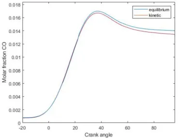
Thanks to the kinetic approach, a better prediction of the CO emission can be obtained. The difference with respect to quilibrium based approach is highlighted in figure 2.7: this gap enlarges as the engine regime increases.

Figure 2.7: Predicted in-cylinder CO molar fraction versus crank angle in a syngle cylinder SI engine. A/F: 13.0; regime: 10000 rpm

The approach explained so far is more complex to apply, thus a semi-empirical method has been developed in order to simplify the problem. The Baruah method states that the actual concentration of CO is lower than the max-imum value in the cylinder and higher than the equilibrium one. Starting from that, the following expression has been proposed:

CO = COeq+ fCO· (COmax− COeq) (2.2.4)

The term fCO is a calibration factor that varies from 0 to 1: if fCO = 0 the

CO emissions are equal to the equilibrium value; if fCO = 1 they are equal

2.3

Nitrogen oxides

2.3.1

Formation

Three main mechanisms cause the nitrogen oxides formation in thermal ma-chines:

• Thermal NOx: high temperature promotes the dissociation of N2 from

air, followed by its oxidation;

• Fuel NOx: nitrogen embedded into the fuel, bounded to other

com-pounds, dissociates and oxydates;

• Prompt NOx: in the flame region, nitrogen reacts directly with

hydro-carbon radicals.

All of these mechanisms are based on kinetics of reactions, since equilibrium condition cannot be assumed. The last two sources of NOx are negligible in

intenal combustion engines: nitrogen is not contained into the fuel exploited in such machines; the prompt mechanism is instead relevant just at low tem-perature, as the thermal dissociation is hindered.

To conclude, thermal dissociation and oxidation represent the main cause of NOx formation in IC engines.

The most widely accepted mechanism to describe NO formation in IC engines is the Zeldovich model:

N2 + O NO + N (2.3.1)

N + O2 NO + O (2.3.2)

The driving force of these reactions is the high temperature in the flame re-gion. If the temperature exceeds 2000 K, dissociation of nitrogen molecules occurs, thus activating Zeldovich mechanism reactions. Earlier burning ele-ments are those that reach the highest temperature, since they are further compressed by later burning ones: a NOx concentration gradient headed

to-wards the spark plug is formed inside the combustion chamber. The rate of reaction of NO is given by [16]:

d[N O] dt = + k

+

1[O][N2] + k2+[N ][O2] + k3+[N ][OH]

− k₁−[N O][N ] − k−₂[N O][O] − k₃−[N O][H]

(2.3.4)

A simplifying assumption adopted states that the change in atomic nitrogen concentration is a quasi-steady process:

d[N ] dt = 0

This assumption is true for most combustion cases, except in extremely fuel rich environment [20].

Thus, equation 2.3.4 can be reduced to: d[N O] dt = 2k + 1 [O][N2] (1 − k − 1k − 2[N O]2 k₁+k₂+[N2][O2]) (1 + k − 1[N O] k+₂k+₃[O2][OH]) (2.3.5)

The resulting equation highlights the two parameters influencing NO emis-sions: NO formation rate increases with oxygen concentration, as well as with temperature: beyond 2200 K, for every 90 K temperature increase, NO

production rate doubles [20]. In particular, temperature plays the most im-portant role, since below 1800-2000 K the reaction rate of N2 dissociation

becomes negligible.

Thus, the main engine specifics affecting NOx emissions are [1]:

• Air/Fuel ratio;

• Spark advance versus TDC;

• Exhaust Gases Recirculation (EGR); • Engine rotational speed and load; • Compression ratio and supercharging.

Focusing on the first item, the in-cylinder maximum NOx concentration

oc-curs for a slightly lean mixture, with equivalence ratio Φ = _αα

s= 0.9. Indeed,

despite the temperature peak is achieved with slightly rich mixture, with complete fuel consumption, oxygen availabilty is important to produce ni-trogen oxydes.

By increasing the spark advance, instead, the combustion process happens closer to TDC, with consequent higher pressure and temperature peak, thus higher NOx emissions.

Finally, a brief explaination of EGR influence on this pollutant is provided. At partial load, as EGR percentage increases up to 15-20%, we get two positive contributions: the mixture is cooled down, and oxygen availability decreases, thus NOx emissions are reduced.

2.3.2

Prediction Model

Zeldovich extended 6 reactions model

The Zeldovich extended 6 reactions model is the simplest NOx predictive

approach implemented in Gasdyn. The involved reactions are:

N2 + O NO + N (2.3.6) N + O2 NO + O (2.3.7) N + OH NO + H (2.3.8) N2O + O 2NO (2.3.9) N2O + O N2 + O2 (2.3.10) N2O + H N2 + OH (2.3.11)

The substantial difference with respect to the simpler three reactions Zel-dovich model is the presence of the intermediate N2O.

N2O rate of reaction can be expressed as:

d[N2O] dt = + k − 4[N O] 2 + k−₅[N2][O2] + k6−[N2][OH]

− k₄+[N2O][O] − k5+[N2O][O] − k6+[N2O][H]

(2.3.12)

Since the characteristic formation and destruction time scales of N2O are

lower than NO, quasi-steady state for N2O can be assumed [20]:

d[N2O]

Thus, N2O can be expressed as:

[N2O] =

k₄−[N O]2_{+ k}−

5[N2][O2] + k6−[N2][OH]

k₄+[O] + k+₅[O] + k₆+[H] (2.3.13) Finally, we can express the NO reaction rate in the 6 reactions model:

d[N O] dt = + k

+

1 [O][N2] + k2+[N ][O2] + k3+[N ][OH] − k −

1[N O][N ]

− k−₂[N O][O] − k₃−[N O][H] + k+₄[N2O][O] − k4−[N O] 2

(2.3.14)

where [N2O] can be computed from 2.3.13.

Zeldovich super-extended 67 reactions model

This approach includes a variety of additional species with respect to the default simulation model.

In particular, the following 22 species are considered: N2, O, N, O2, OH, H,

N2O, HO2, NO, NO2, O3, NO3, HNO, NH, H2, H2O, Ar, H2O2, NH3, NH2,

N2H3, N2H2.

It is experimentally observed that the production and destruction time scales for N, NH, NH3, NH2, N2O, HNO are lower than NO ones, but higher than

N2, O, O2 and OH. Therefore, a system of 7 reaction rate equations has to

be solved, in order to get [NO], as stated by [8].

The model intrinsic complexity limits its use to extreme conditions, such as to calibrate the simpler scheme.

2.4

Unburned hydrocarbons

2.4.1

Formation

The emission of unburned hydrocarbons is the result of an incomplete com-bustion. Several engine design parameters influence the HC level in the exhaust, such as [1]:

• Air/Fuel ratio;

• Spark advance with respect to TDC;

• Surface/Volume ratio and combustion chamber shape; • Amounts of deposit on the walls;

• Engine rotational speed and load; • Cooling system efficiency;

• Overlap angle;

• Pressure drop due to the exhaust system.

The first two parameters affecting HC emissions have a stronger influence than the others.

Focusing on Air/Fuel ratio, it has an important effect on the level of HC emissions, since it controls the oxygen availability. The minimum value, as we can see in figure 2.8, is reached for a slightly lean mixture. Rich mixtures result in lack of oxygen, while very lean ones in poor combustion quality.

Figure 2.8: [1] Pollutants concentration against relative Air/Fuel ratio coef-ficient

As for the spark advance, instead, it influences the amount of HC that can be post-oxidized. If the spark advance decreases, the combustion process is delayed and it continues during the expansion stroke. The HC that have escaped from the primary combustion are mixed with the burned gases and oxidized. Even if a small reduction of the spark advance may be beneficial in terms of HC emissions, it is detrimental for engine performance as well.

Picture 2.8 shows another important concept: HC emissions have to be reduced not only because they cause environmental pollution, but also to increase engine efficiency: the profile of Brake Specific Fuel Consumption (BSFC) has the same trend as HC one.

Several mechanisms bring to the formation of HC: in this section it is provided a brief explaination of the main causes, while in the next chapter the focus is entirely on scavenging.

• HC from scavenging

During the valve overlap period, as the scavenging of the combustion chamber takes place, part of the fresh mixture could directly flow from the intake to the exhaust valve, so that the embedded unburned fuel is emitted. This is the most important phenomenon that causes HC emissions.

• HC from crevices

Fuel mass stored inside cylinder crevices causes HC formation, since the flame cannot reach it. After the flame has passed, only part of the fuel is post-oxidized during the expansion stroke.

• HC from oil film

The oil film on the cylinder wall can absorb the fuel hydrocarbons when the HC partial pressure is high, then release them during expansion stroke, as pressure decreases.

• HC from quenching

Quenching is a term that describes the flame extinction close to the cylinder walls or on the piston crown. The temperature on these sur-faces is much lower than inside the combustion zone: when the flame approaches them, if the temperature is too low, the combustion may not occur. This phenomenon is particularly frequent after a cold start of the engine.

• HC from blow-by flux

A small portion of the cylinder mixture may flow through the rings and go into the engine basement. Then it is directly dispersed into the environment, causing HC emissions.

2.4.2

Prediction Model

In this section we are going to discuss the approaches to predict the HC emissions from crevices and oil film, while in the next chapter we will focus on the analysis of the scavenging model and the evaluation of HC due to short circuit, mixing and inlet backflow.

HC from crevices

Gasdyn code evaluates per each step the flame front radius and the distance between spark-plug and crevices: by comparing them, it can be understood whether the unburned fuel is going to be oxidized or not. The mass inside the crevices is evaluated by means of the following equation:

mc=

pVcM

RTp

(2.4.1)

where:

p: combustion chamber pressure [P a]; Vc: cervices volume [m3];

M : fresh mixture molar mass [g/mol]; R: universal gas constant [J/molK]; Tp: piston temperature [K].

The mass variation in time is: dmc dt = VcM RTp · dp dt (2.4.2)

The main assumptions are:

• mass temperature is equal to piston temperature (contact thermal boundary condition);

• the spark-plug is in the cylinder head, in the center;

• the flame front has a spherical shape with its center in the spark-plug.

HC from oil film

In order to evaluate the emission of unburned hydrocarbon from the oil film, since mass transfer is diffusion controlled, a 1D differential equation for mass conservation has to be solved:

∂YHC ∂t − D ∂2_Y HC ∂x2 = 0 (2.4.3) where:

YHC: fuel mass fraction in the oil film [kgf/kgo];

x: distance from cylinder wall [cm];

D: coefficient of diffusion in the solvent [cm2/s].

Cylinder 2D space has to be divided into a number of small elements in both radial and vertical direction. This approach allows the code to solve the equation and to evaluate the emission of HC.

Scavenging model

3.1

Introduction

In the previous chapter, pollutants emission modelling has been described. As for unburned hydrocarbons sources, three main phenomena have been mentioned: crevices, oil film and scavenging. The first two contributions have been properly analyzed so far, while scavenging is dealt with in this chapter.

Scavenging model is capable to capture the emissions of HC during the valve overlap period, mainly due to the following phenomena:

• short circuiting of the unburned mixture directly through the exhaust port;

• mixing between unburned and burned mixtures; • inlet backflow.

The main aim of this thesis is to highlight the magnitude of the scavenging process on the overall HC emissions of spark ignition engines. Indeed, the

original version of the Gasdyn code is not able to capture all the complex fluid dynamic phenomena contributing to HC emissions during the valve overlap period.

Thus, in the follow-up of this dissertation the focus will be on the model de-scription and implementation, as well as on the comparison of the calculated results with the experimental ones.

3.2

Cylinder scavenging process

As the crank angle varies, the mixture contained into the engine cylinders changes both its mass and its composition.

Figure 3.1: Four strokes engine gas exchange process [9]

At the exhaust valve opening (EVO) , typically 40◦- 60◦ before BDC depend-ing on the specific engine, the burned gases flow through the exhaust duct, decreasing the in-cylinder pressure and temperature. This process occurs during the last part of the expansion stroke and the whole exhaust stroke, since exhaust valve closing (EVC) happens at around 370-400 crank angle degrees, i.e. the beginning of intake stroke.

Nearly at the end of the exhaust stroke, around 10◦- 40◦ before TDC, the intake valve opens (IVO). The fresh charge from the environment is delivered to the cylinder, flowing through the intake port during the whole intake stroke and the beginning of the compression stroke. In-cylinder pressure increases, as long as the overall mass contained. Intake valve closing (IVC) typically takes place 40◦- 80◦ after BDC.

As shown in picture 3.2, valve overlap period may occur in common engines. During this crank angle interval, which can vary as function of the engine regime and load, intake and exhaust systems may interact:

• If the fluid inertia is strong enough, fresh charge may short circuit the cylinder, flowing directly through the exhaust port.

• Burned gases from exhaust ducts can backflow through the intake port, if pressure pulses are favourable: a sort of internal exhaust gases recir-culation (EGR) occurs, with positive consequence on NOx emissions,

as discussed in the previous chapter.

The short circuit does not have any impact on unburned hydrocarbons emis-sions in direct injection engines, such as Diesel and modern spark ignition (GDI) ones, since only air is lost. However, in indirect injection engines a relevant amount of HC is emitted during valve overlap period due to short circuit.

Figure 3.2: Circular diagram with opening and closing time of intake and exhaust valves [9]

3.2.1

Original cylinder model

The original model for the gas exchange process implemented in the Gasdyn code describes the engine cylinder by means of a single zone approach. There is no distinction between residuals and unburned, since perfect mixing is assumed: in this way both the inlet and the outlet fluxes contribute directly to the variation of the cylinder mass and composition. This model is quite well predictive of CO and NOx emissions, as well as HC from crevices and

oil film. Its weakest point concerns the HC emitted during the valve overlap period, since the short circuit of the fresh charge cannot be captured.

3.2.2

Scavenging submodels

Three different submodels can be adopted to properly describe the scavenging process:

1. perfect displacement; 2. homogeneous mixing; 3. pure short circuit;

Picture 3.3 shows their application on a two stroks engine, where the mag-nitude of scavenging is much higher.

Figure 3.3: Scavenging submodels [9]

All of these models will be discussed in the following, starting from the first, which represents an ideal process.

In order to describe scavenging process, three coeffiecients are introduced: • volumetric efficiency λv=_{displaced volume · ambient density}mass of air trapped per cycle =m_ma_t

• scavenging coefficient λs=mass of air delivered to the cylinder_{displaced volume·ambient density} =m_ms_t

where mt is the reference mass.

Despite the last two indexes are typically adopted in two strokes engines, they can be exploited also in four stokes to properly describe the phenomenon. Perfect displacement

Perfect displacement represents an ideal situation: fresh charge entering from the intake port would displace the combustion products without any mixing. If the incoming mass msdoes not exceed the reference one mt, the mass flux

leaving the cylinder through the exhaust port is entirely composed by burned gases: all the mass entering is trapped inside the cylinder for the combustion process. If instead the mass ms exceeds the reference value mt, the surplus

is discharged through the exhaust port, causing HC emissions. Picture 3.4 shows the trend of λv versus λs.

These concepts may be summarized as: λs ≤ 1 → λv = λs and λtr = 1 (3.2.1) λs > 1 → λv = 1 and λtr = 1 λs (3.2.2) Homogeneous mixing

According to [1], homogeneous mixing is ”a quite pessimistic model of the real behaviour”. In order to describe this assumption, the following terms are introduced:

• ma: fresh charge retained into the cylinder;

• mr: residual mass retained into the cylinder;

• mm: overall cylinder mixture mass;

• dms: scavenging mass element;

• dmm: outgoing mass element of mixture;

• dma,out: outgoing mass element of fresh charge.

In a generic time instant t, the overall cylinder mass mm is equal to the

summation of the first two terms:

mm = ma+ mr (3.2.3)

As gas exchange process goes on, the mixture mass mmvary both its quantity

and composition. Focusing on an infinitesimal interval dt, the mass of fresh charge retained in that time step in the cylinder can be expressed as:

Since homogeneous mixing is assumed, the composition of the mixture leav-ing the cylinder in the infinitesimal time step is the same as the overall control volume: dma,out dmm = ma mm (3.2.5)

Thus, combining (3.2.4) and (3.2.5) we get:

dma = dms−

ma

mm

dmm (3.2.6)

The model can be visualized in picture 3.5

At this point, two more assumptions are introduced:

1. the cylinder pressure variations during valve overlap period when scav-enging process occurs are so low that gas compressibility may be ne-glected;

2. the piston motion around BDC is small, so that the cylinder volume can be considered constant in time, equal to its mean value Vm,cyl.

Starting from this latter hypothesis, we can express Vm,cyl as:

Vm,cyl=

mm

ρm

Therefore, the volume of gas entering in interval dt equals the leaving one: dms ρs = dmm ρm Equation (3.2.4) becomes: dma = dms[1 − ( ρm ρs )(ma mm )] = dms[1 − ma ρs Vm,cyl ] (3.2.7)

The ordinary differential equation obtained can be solved by means of vari-ables separation. Finally we get to the following form:

ma = ρs Vm,cyl[1 − exp(−

ms

ρs Vm,cyl

)] (3.2.8)

contained into the cylinder undergoes and exponential increase, tending to the limiting value ρsVm,cyl. Therefore, this model represents the most

un-favourable situation to remove all the residuals from the cylinder, since a theoretical infinite mass of fresh charge would be required to accomplish the full scavenging of the combustion chamber. Moreover the incomplete scavenging causes a worsening of the combustion process, since part of the mixture partecipating to the new thermodynamic cycle has already been burned.

This situation can be represented by rearranging equation (3.2.8). In partic-ular, by dividing both sides by the reference mass mt=ρaV and expressing

ms as ms=λs mt, we get: ma mt = (ρs Vm,cyl ρaV )[1 − exp(−λs ρaV ρs Vm,cyl )] (3.2.9)

By introducing the non-dimensional coefficient Ψ = ρs Vm,cyl

ρaV , we get the

dimensionless form of the cylinder filling law: λv = Ψ[1 − exp(−

λs

Ψ)] (3.2.10)

Ψ is typically close to 1, according to [1]: in that special case, we can represent the trend of the function λv = 1 − exp(−λs) in figure 3.6:

Figure 3.6: Cylinder filling in homogeneous mixing scavenging model To complete the analysis, the trapping efficiency λtr can be expressed by

substituting equation (3.2.10) into λtr definition:

λtr = λv λs = (Ψ λs )[1 − exp(−λs Ψ)] (3.2.11)

In the end, we can identify the working area where real cases stay into, as shown in green in figure 3.7.

Figure 3.7: Volumetric and trapping efficiency versus scavenging coefficient Pure short circuit

Pure short circuit represents the worst situation of scavenging process. Fresh mixture, after displacing all the combustion products on its pathway, flows directly through the exhaust port, without any mixing with the burned gases. A schematic of this phenomenon is shown in figure 3.8.

There are two main consequences of this situation: 1. high emission of unburned HC;

2. low volumetric efficiency.

3.3

Scavenging model

3.3.1

Fundamental assumptions

In order to investigate the gas exchange process, a four zones model is adopted to describe the cylinder-ducts system: each control volume has vari-able mass and composition as function of the crank angle. As shown in picture 3.9, we can distinguish the following zones:

1. cylinder unburned zone; 2. cylinder burned zone; 3. inlet duct;

4. exhaust duct;

We can associate to each control volume its mass:

1. mASP, cumulative mass in the intake duct due to the inlet backflow;

2. mDIS, cumulative mass in the exhaust duct, due to the regular exhaust

port discharge;

3. mU, cylinder unburned region mass;

4. mB, cylinder burned region mass.

As for the fluid modelling, the simplest assumption is the perfect gas, with constant specific heats. However, each zone is considered as composed by an ideal mixture of ideal gases. This choice is dictated by the requirement of emission tracking in the exhaust system: in order to assess a crank angle dependent analysis of both concentration and mass flow rate of the species in the pipes, the transport of species has to be implemented. A further benefit of this assumption is that the specific heat at constant pressure is function of both temperature and composition, so that thermodynamic calculations are more precise.

14 species are tracked inside the pipes by the code:

• 11 reacting species: N2, O2, CO2, H2O, CO, H2, H, O, OH, NO and

FUEL. This latter can be arbitrary chosen as an input; • Argon as inert species;

• 2 unburned hydrocarbons species: C3H6, C3H8

Their concentration vary with the crank angle, according to gas exchange phenomena and combustion process.

Finally, a brief mention to the sign convention of flows through the cylinder ports is provided. For each angular step, the inlet and exhaust mass flow

rates are computed by proper functions already implemented in the code. In the following picture, their sign convention is shown.

We can identify four primary fluxes among the zones: 1. Intake → Unburned;

2. Burned → Exhaust;

3. Unburned → Burned: mixing flux; 4. Unburned → Exhaust: short circuit flux.

The first three fluxes happen between adjacent control volumes. Specifically, the first two link the cylinder volume with ducts, representing gas exchange through the valves, while the third one occurs entirely inside the cylinder. The short circuit flux, instead, accounts for the fresh mixture bypassing the cylinder volume, by flowing directly through the exhaust port.

Furthermore, two secondary fluxes can be modelled: 1. Intake → Burned;

2. Unburned → Exhaust.

The last contribution, despite being directed as the short circuit one, has a different meaning: it represents the mass flow rate discharged to the exhaust duct directly from the unburned zone when the burned mass is null.

Figure 3.11: Four zone model fluxes [11]

Picture 3.11 distinguish four kind of fluxes, represented by arrows: • Primary fluxes of fresh mixture are portrayed in blue;

• The only primary flux of burned gases is in orange; • The two secondary fluxes are represented in black; • The fuel injected is in green.

Focusing on the last item, even if fuel injection is indirect, the Gasdyn code models it as if it was direct. Indeed, fuel does not pass through the intake valve, but it is directly submitted to the cylinder. The difference with respect to direct injection consists in the timing: direct injection occurs when the exhaust ports are closed, while Gasdyn injection starts when the inlet air

3.3.2

Mass fluxes

The new model implemented in the Gasdyn code takes into account both mixing and short circuit of the fresh charge. Inside the cylinder, three macro species are modelled: air, fuel and residuals.

The starting point consists in assuming that, if the calculation angle α is lower than IVO, the cylinder mass is entirely made of residuals, located in the burned zone. Both fuel and air are not present inside the cylinder so far, since the combustion has taken place. Moreover, the mass of the unburned region is null.

As the calculation angle α exceeds IVO, the scavenging process is modelled. Firstly, all mass fluxes are computed, starting from primary ones; then mass balances are revised.

• Short circuit

Short circuit is represented as a flux from unburned to exhaust zone. In order to have this phenomenon, the following conditions have to be respected simultaneously:          dmIN > 0 dmOU T > 0 mU > 0

The first two statements highlight that the overall flux must be headed from the intake pipe to the exhaust one, without backflow effects; the last one, instead, means that no short circuit happens if only burned gases are present within the cylinder.

The short circuit mass flux in the time step is expressed as:

The through-flow mass flow rate is function of ports fluxes and a co-efficient depending on the flow turbulence intensity, whose calibration will be properly discussed in the next sections.

• Mixing

Mixing is represented as a flux from unburned to burned zone. It can be modelled as:

dmM IX = KM IX · (dmIN − dmSHC) (3.3.2)

The following conditions have to be respected:          dmIN > 0 mU > 0 mB > 0

In order to properly understand them, it has to be noticed that mixing is irreversible: dmM IX must be positive, so dmIN > 0. The last two

conditions are strictly related to the nature of this phenomenon: mU >

0 is required to provide fresh charge to the burned zone; mB has to be

positive, otherwise unburned mass would self-mix.

Equation 3.3.2 states that mixing flux is limited by short circuit one: being both KM IX and KSHC at most equal to unity, the following

inequality is verified at any time step, during valve overlap period: dmSHC + dmM IX ≤ dmIN (3.3.3)

Thus, the excess of mass entering with respect to the one leaving the unburned region contributes to increase mU.

Furthermore, for both mixing and short circuit, if one of the conditions is not satisfied, then the correspondent mass flow rate is set equal to zero. Short circuit and mixing fluxes are then partitioned among air, fuel and residuals, depending on the mass fractions in the unburned control volume:

dm(j)_SHC = m (j) U mU · dmSHC dm(j)_{M IX} = m (j) U mU · dmM IX

where apex j represents the j-th macro-specie.

To conclude the calculation of primary fluxes, the contributions at the ports have to be discussed.

• Inlet flux

In order to calculate inlet flux, different situations have to be examined. – Firstly, we consider the case when the incoming mass flow rate dmIN is negative, which represents backflow from the cylinder to

the intake pipe. Due to this phenomenon, the composition of the leaving stream is detemined by the unburned zone. Obviously, the flux is non null if the unburned mass is greater than zero. This case can be summarized as:

   dmIN < 0 mU > 0 dm(j)_U,IN = m (j) U mU · dmIN (3.3.4)

species: air, fuel or residual. In this case, also, the mass flow rate of injected fuel represented in figure 3.11 is null: dmF U EL = 0.

– When there is cumulative mass in the intake pipe, due to back-flow in previous time steps, it is preferentially sent to the cylinder, rather than environmental air. This means that, as the inlet mass flow rate becomes positive, the accumulate in the first zone de-creases until complete depletion. This assumption is reasonable, since the backflow volume behaves as a buffer. The composition of the incoming flux is dictated by the one of the intake zone. The following conditions summarize this situation:

   dmIN > 0 mASP > 0 dm(j)_U,IN = m (j) ASP mASP · dmIN (3.3.5)

Furthermore, as in the previous case, dmF U EL = 0: this statement

satisfies the requirement to keep the Air-Fuel Ratio constant to the fresh charge input value.

– The other possible situation concerning the intake flux to examine is consequential to the previous one: if the mass flows from inlet pipe to cylinder without any buffer to deplete, the composition is fixed by the intake system. In that case, the fuel is injected to satisfy the A/F requirement. These concepts can be expressed as:

  dm_IN > 0 →   dm_IN = dm_A,IN 1

• Outlet flux

The primary flux at the outlet port, named dmB,EX, occurs from burned

zone to exhaust one. Two possible situations may happen, with the following relation in common:

dmB,EX = dmOU T − dmSHC (3.3.6)

– If both the outlet mass flow rate and the overall mass inside the burned zone are positive, then the composition is dictated by the cylinder burned zone:

   dmOU T > 0 mB > 0 dm(j)_B,EX = m (j) B mB · (dmOU T − dmSHC) (3.3.7)

Thus, the model assumes that a portion of dmOU T is due to short

circuit, if present, while the rest is given by dmB,EX.

– If there is backf low, dmOU T is negative; the composition is fixed

by the exhaust duct, provided that an accumulate is available:    dmOU T < 0 mDIS > 0 dm(j)_B,EX = m (j) DIS mDIS · dmOU T (3.3.8)

As anticipated so far, two secondary fluxes are modelled to guarantee the closure of the balances in every cases: they are thought to represent quite unusual but possible situations.

• Inlet secondary flux

By considering inlet port, in case of backflow from cylinder to intake system, the mass flow rate of the j-th macro species has been computed in equation (3.3.4). However, if there is no mass in the unburned region, an alternative has to be proposed. In particular, provided that mB is

positive, which is trivial since either unburned or burned have to occupy the cylinder, the inlet secondary flux moves from burned to intake zone. Its composition depends on the burned region one:

         dmIN < 0 mU = 0 mB > 0 dm(j)_B,IN = m (j) B mB · dmIN (3.3.9)

• Outlet secondary flux

The secondary flux at the discharge port moves from unburned to ex-haust zone: its pathway is the same as short circuit one, but the back-ground is different. Indeed, this flow rate appears as an alternative to normal discharge dmB,EX. If there is no mass to discharge in the

burned region, as for example close to EVC, then the regular flow at the exhaust port is guaranteed by this unburned gas flux:

         dmOU T > 0 mB = 0 mU > 0 dm(j)_U,EX = m (j) U mU · (dmOU T − dmSHC) (3.3.10)

3.3.3

Mass balances

Once all the fluxes have been computed, mass balances are performed: dmIN = dmU,IN + dmB,IN Intake (3.3.11)

dmEX = dmB,EX + dmU,EX + dmSHC Exhaust (3.3.12)

dmU = dmU,IN+ dmU,B+ dmSHC+ dmU,EX U nburned (3.3.13)

dmB = dmU,B+ dmB,EX + dmB,IN Burned (3.3.14)

It has to be noticed that all the previous equations are in algebraic form, meaning that their terms may become negative.

Focusing on fuel macro species in the unburned region, a further contribution due to injection modelling, named dmF U EL, has to be accounted.

The four above mentioned balances are representative of the whole zones. In the code, however, the implementation is different, since equations 3.3.11 to 3.3.14 are applied to the macro species inside the zone. Considering the unburned zone:

m(t+dt)_AIR,U = m(t)_AIR,U + dm(AIR)_U,IN + dm(AIR)_U,B + dm(AIR)_SHC + dm(AIR)_U,EX m(t+dt)_RES,U = m(t)_RES,U+ dm(RES)_U,IN + dm(RES)_U,B + dm(RES)_SHC + dm(RES)_U,EX

Then, the three contributions are joined, to get the whole unburned zone mass:

m(t+dt)_U = m(t+dt)_{F U EL,U} + m(t+dt)_AIR,U+ m(t+dt)_RES,U The same procedure is carried out for other control volumes.

No mention to chemical species has been done so far. Since macro species and control volumes mass balances have been performed, the amount of each chemical species inside the cylinder can be obtained. It is important to notice that at this point no further distinction among unburned and burned region is done, since the aim is to calculate the overall mass of the j-th spcies inside the cylinder at the generic time step.

• Air is assumed to be composed by 79% nytrogen and 21% oxygen, on molar basis. Therefore, the correspondent percentage of the all m(t+dt)_AIR,U, on mass basis, is allocated on them.

• Residuals are divided among all the species according to the combustion chamber composition calculated at EVO.

• Fuel is entirely allocated on its correpondent species. As for example, is it shown the calculation of nytrogen mass:

m(t+dt)_N 2 = m (t+dt) AIR · 0.79 · M MN2 M MM IX · (1 − EGR%) + m (t+dt) RES ∗ yN2, RES