Autore:
Domenico A. Fittipaldi ____________________
Relatori:
Prof. Marco Luise ____________________
About the Use of Adaptive Antennas
in 60 GHz UWB-OFDM
Personal Area Network Transceivers
Anno 2008
UNIVERSITÀ DI PISA
Scuola di Dottorato in Ingegneria “Leonardo da Vinci”
Corso di Dottorato di Ricerca in Ingegneria dell’Informazione
Abstract
The recent opening of unlicensed spectrum around 60 GHz has raised the interest in designing gigabit Wireless Personal Area Networks (WPANs). Since at 60 GHz the signal attenuation is strong, this band is basically suitable for short range wireless communications. It is understood that directional antennas can be employed to compensate for the path loss and combat the waste of power due to the scatter phenomena characteristic of these high frequencies.
This thesis studies the use of adaptive array systems in 60 GHz Ultra Wide Band-Orthogonal Frequency Division Multiplexing (UWB-OFDM) personal area network transceivers. The study has been conducted by simulations and theoretical analysis. Two sensor arrangements have been considered, the Uniform Linear Arrays (ULA) and the Uniform Circular Arrays (UCA), in the simple case of the Line of Sight (LOS) transmission scenario.
On the one hand we have designed a IEEE 802.15.3c Medium Access Control (MAC) phased-array controller throughput using Direction of Arrival (DOA) estimation to perform beamsteering. We have simulated the MAC controller with the network simulator ns-2. The impact of the array controller performance onto the achievable throughput of the wireless links has been studied to draw the requirements about the standard deviation of the DOA estimator.
On the other hand, we have found the Cramér-Rao Bound (CRB) for DOA estimation of impinging 60 GHz OFDM sources. The requirements of the standard deviation of the DOA estimator are analysed against the CRB for DOA to validate the design of the directional 60 GHz UWB-OFDM transceivers.
The comparison reveals that directional 60 GHz UWB-OFDM transceivers can achieve high wireless throughput with a number of pilot subcarriers and for a Signal to Noise Ratio (SNR) operating range typical of next generation WPANs.
I
Summary
Chapter I. Introduction: Millimeter Wave PANs ... 1
1.1 The 60 GHz Challenge... 1
1.2 Smart Antennas Overview ... 3
1.3 Advantages of Directional Antennas for 60 GHz WPANs ... 4
1.4 Adaptive Arrays Controller... 6
1.5 Goal and Contributions ... 7
1.6 Outline ... 8
Chapter II. Antenna Arrays Fundamentals ... 11
2.1 Array Processing ... 11
2.3 Reference Antenna System ... 14
2.4 Narrow Band Antenna Model ... 16
2.5 Uniform Linear Array Model ... 16
2.5.1 Array Factor of ULA Systems ... 19
2.6 Uniform Circular Antenna Model... 25
2.6.1 Array Factor of UCA Systems ... 26
2.7 Antenna Directivity. ... 28
2.7.1 Directive Gain of ULA Systems... 29
2.7.2 Directive Gain of UCA Systems ... 29
2.8 Beamsteering... 30
2.8.1 Beamsteering of ULA Systems... 30
2.8.2 Beamsteering of UCA Systems ... 33
2.9 Half Power Beamwidth of ULA Systems ... 35
Chapter III. Simulation Analysis with IEEE 802.15.3c MAC ... 37
3.1 General Description of IEEE 802.15.3 ... 37
3.2 Adapting IEEE 802.15.3c MAC for the Use of Phased Array Antennas... 41
3.2.1 DOA Estimation on the PHY Preamble... 41
3.2.2 Frame Driven Beamsteering in IEEE 802.15.3c MAC... 43
3.3 Simulation Background... 46
II
3.5 Simulations Analysis with UCA Systems... 54
Chapter IV. CRB for DOA Estimation of Narrow Band Data Signals ... 57
4.1 CRB on DOA Estimation of Narrow Band Signals. ... 57
4.2 Derivation of the FIM from the Sufficient Statistic ... 60
4.3 CRB for DOA with ULA Systems ... 61
4.4 CRB for DOA with UCA Systems... 64
4.5 Extension of the Observation Time to more Symbol Intervals ... 66
4.6 Derivation of the FIM from the Continuous Time Observation Space... 67
4.7 MCRB: Estimation with Unknown Data Symbols... 67
Chapter V. CRB for DOA of OFDM Data Signals ... 71
5.1 CRB of Parameter Estimation with Waveforms having Orthogonal Derivatives ... 71
5.2 DOA Estimation of OFDM Signals over AWGN Channel ... 75
5.2.1 Numerical Example: IEEE802.15.3c OFDM ... 81
5.2.2 Comparison between OFDM Signals and Monocarrier Signals... 84
5.3 DOA Estimation of OFDM Signals over Frequency Selective Channel ... 87
5.4 Comparison of the CRB for DOA with the Simulation Analysis Results... 93
Conclusions and Developments ... 96
Appendix A: Analytic White Gaussian Noise... 99
Appendix B: FIM Computation ... 101
B.1 Derivation of the FIM from the sufficient statistic z of narrow band signals ... 101
B.2 Derivation of the FIM from the analytic signal y(t ) of narrow band signals... 106
B.3 Derivation of the FIM for OFDM Signals in the case of Frequency Selective Channels ... 111
1
Chapter I. Introduction: Millimeter Wave PANs
1.1 The 60 GHz Challenge
Wireless personal area network (WPANs) are used to convey information over relatively short distances among a relatively few participants through connections involving little or no infrastructure. This allows, small power efficient, inexpensive solutions to be implemented for a wide range of wireless devices. The millimeter-wave PANs will be the Gbps evolution of the wireless personal area network technology. The first WPAN standard is IEEE 802.15.1 which is commonly known with the name of Bluetooth, while the latest standard of this wireless family is IEEE 802.15.3a which operates in the 2.4 GHz Industrial Scientific and Medical (ISM) Band [1]. The recent opening of massive unlicensed spectrum around 60 GHz fosters the design of WPANS with a target date rate up 5 Gbps whilst the ones operating at 2.4 GHz reaches 55Mbps at most. The abundance of bandwidth available and the signal propagation phenomena typical of these frequencies make the 60GHz band appealing for the even growing market of the short range wideband applications when the other unlicensed bands are or are becoming crowded.
Two organizations that have driven the 60 GHz radios are the IEEE 802.15.3 standard body [2] and the WiMedia Alliance [3], an industrial association. The IEEE 802.15.3 Task Group 3c (IEEE 802.15.3c) is developing a mm-wave-based alternative physical layer to the existing 802.15.3 WPAN standard IEEE-Std-802.15.3-2003. The WiMedia Alliance is pushing a 60GHz WPAN industrial standard based on Orthogonal Frequency-Division Multiplexing (OFDM) [4]. Figure 1. 1 and Table 1. 1 show the worldwide availability of bandwidth around 60 GHz and the most recent regulatory results for this band.
2
Figure 1. 1- Spectra available around 60 Hz
57 58 59 60 61 62 63 64 65 66
59.4 62.9
Table 1. 1 - Emission power requirements
Region Output Power Other Considerations
Australia Canada and USA
10 mW into antenna 500 mW peak
150 W peak EIPR min. BW = 100MHz Japan 10 mW into antenna
+50, -70% power change OT and TTR 47 dBi max. ant. Gain
Europe + 55 dBm EIPR min. BW = 500 MHz
The core of the design of the millimeter WPANs lies at the physical layer (PHY) and the Medium Access Control (MAC) layer. At PHY the wireless channel reliability is the issue to face in order to make the high data rates of the millimetre WPANs realistically achievable. Probably, OFDM is the most suitable technique for high speed data transmission at 60 GHz. This technique partitions a high frequency selective wideband channel to a group of nonselective channel, which makes it robust against large delay spreads while preserving orthogonality in the frequency domain. Another property of OFDM that makes it very attractive for wideband applications is its easy scalability to different environment, bandwidth and bit rates. Our study assumes OFDM as the data modulation technique of the millimeter WPANs [2].
Another important feature of these frequencies is the strong attenuation that the signals undergo in free space propagation and trough materials. Directional antennas are the candidate PHY capability to compensate for the path loss. In Section 1.3 we review the Smart Antennas in general and in
3
Section 1.3 we discuss the potential benefits of the adaptive antennas in the specific case of the mm-wave WPANs by taking into account the features of the wireless channel at the frequencies of interest.
On the other hand, the use of directional antennas raises the problem of designing the beamforming intelligence that steers the main lobe of the antenna to point the right direction at the right time. The design usually involves PHY and MAC, although it could touch other network layers at the cost of more end-to-end delay in the case of data delivery failure and more compatibility problems among different standards. In Section 1.4 we discuss the guidelines of designing adaptive array controllers in more detail.
1.2 Smart Antennas Overview
Smart antennas are directional antennas that use signal processing both in space and time to sense the neighbour electromagnetic environment and to adjust their radiation patterns subsequently according to a given transmission\receive strategy. This mechanism through which the wireless devices become aware of the surrounding environment and react to it when transmitting\receiving constitutes the intelligence of the smart antennas. This intelligence is usually categorized into: Switched Beam Antennas and Adaptive Arrays [5].
• Switched Beam Antennas are designed with a fixed set of radiation patterns. This type of smart antennas can be created by using multiple directive elements each pointing towards different sectors. Basically, the outputs of the radiation patterns of the directive elements are continuously sampled, and the output statistics are composed by selecting (maximum signal) or combined (maximum ratio, equal gain) the output samples. Perfect match between the antenna beams and direction of arrival is realized only in a limited number of directions, those of the single antenna patterns. When plotting the received signal strength versus the Direction of Arrival (DOA), one notices that the plot
4
marks the antenna pattern with even nulls in the nulls of the antenna pattern. This roll-off behavior is known as scalloping.
• Adaptive Arrays are antenna systems where the signals at the input(output) of the antenna elements are multiplied by complex weights that are called weighting elements. These coefficients can be controlled both in amplitude and in phase by an array processor network. If the array processor is designed to control the phases of the signals at each array element but not their magnitudes, the adaptive array is specifically called Phased Array. Phased Arrays provide beamsteering only, that is, the main array beam is steerable in any direction. If the array processor control the amplitudes of the weighting elements as well, the adaptive array system is capable of performing beamforming which is beamsteering and null placing together. Nulls can be placed in the look angles of interfering sources.
Switched-beam antennas are cheaper than adaptive array antennas but the later outperform the former in co-channel interference spatial filtering and direction tracking. This difference is of great importance in mobile applications.
1.3 Advantages of Directional Antennas for 60 GHz WPANs
As for the matter of power, there two main points that is worth highlighting. Array antenna systems relax the requirements for power amplifiers and enlarge the operational coverage of the radio link with respect to isotropic antennas.
According to reports from BWRC, CMOS amplifier gain at 60 GHz is below 12 dB [6], which raises a concern about limited transmitted power. If each branch can emit a certain amount of power, an M-branch transmitter can emit roughly 20log10(M) more power compared to the case of a single
antenna transmitter [7].
On the other hand, the radio coverage increases because the random multipath reflections are suppressed and the power is focused in one
5
intended direction. This, on the one hand, reduces the delay spread with respect to omni antennas. On the other hand, a comparable spatial outage reduction would be highly power consuming in the 60GHz band if performed by omni antennas. In fact the free space path loss of the millimeter waves is (60/5)2 (21.6dB) times the one at 5 GHz and (60/2.4)2 or (27.96 dB) higher than that at 2.4 GHz. High gain directional antennas compensate for the high propagation loss with the antenna gain instead of increasing the power emission. This also limits the generation of co-channel interference. The attenuation of the millimeter waves is also strong trough materials. It is understood that walls of a building act like reliable cell boundaries and WPANs in the 60GHz band will be deployed as in-room, -corridor or -hall cells with hot spot communications.
Another advantage of having a set of antenna elements comes with the application of diversity techniques to resolve the dominant path(s) in a space-time domain for the purpose of improving the link quality/reliability. Diversity antenna schemes require low cross correlation among the diversity channels. In spatial diversity, the cross correlation of the signals received at the array elements is a function of the array element spacing and the power angle profile. Placing the array elements at the distance of many times the wavelength (λ=5mm at 60 GHz) creates low correlation among the channels of the antennas composing the array.
The replicas of the signal may be also uncorrelated in the case of a significant angle spread so that multiple antenna beams receive distinct paths. Angle diversity is expected to provide significant gain improvement in rich scatter environments. In [8] it has been shown that at 60 GHz the angular spread is quite rich for room and obstructed indoor propagation while for Line of Sight (LOS) applications the LOS component is 10 dB above the first order reflections if no strong reflectors are present. In this case Array Processing can be applied to acquire the LOS direction in order to establish directional communication by practicing beamsteering or more
6
in general beamforming. Beamforming increases the network throughput by reducing the interference generation/affection in unintended directions.
1.4 Adaptive Arrays Controller
The design of smart antennas controllers is considered as part of the overall design of the MAC protocols, and the realizable gains of smart antennas for a specific network depend on the control algorithms in use. Lots of work can be found in the literature about the basic mechanisms of employment of the smart antennas in WLANs and Mobile Ad Hoc Networks (MANETs) for the purpose of reducing the typical collision rates of many contention-based MAC access protocols like Aloha, CSMA, CSMA/CA and TDMA [9 - 19].
The advantages of the smart antennas come with the narrow beam signal transmission and/or reception. The main issue related to such narrow beams consists in the knowledge of the pointing direction and in the coordination of antenna steering at both ends prior to accomplishing data transfer among devices. Information about the steering direction toward the intended device is provided through neighbour discovery algorithms which are carried out before the link establishment. There are two basic categories of neighbour discovery techniques with smart antennas in ad-hoc self-configuring wireless networks. One category is composed of those algorithms that do not make use of omni receive operations at any stage. These algorithms are classified as scan-based algorithms, [15] [17]. When using this class of algorithms, devices in the network are synchronized and follow a predefined scan sequence to discover neighbours and point the right direction at the right time. On the other hand, the other class of neighbours discovery strategy is based on the capability provided by the array processing of estimating the angle of arrival of a radio source impinging on the array system. Direction of arrival information is subsequently exploited for space diversity access to the shared radio medium. A thorough characterization of the direction of arrival estimation capability is thus of paramount
7
importance to validate the use of array sensors as realistically viable. In [20] the authors raise the issue of the antenna controller accuracy with highly directive antenna systems. They study the throughput behaviour versus the steering error in a Time Division Multiple Access (TDMA) link and show that significant throughput degradation may be caused by a pointing error of a few degrees. Again the actual benefits of the smart antennas in a specific network depend on the antenna control system whose performance is directly bound to the one of the algorithms of DOA estimation in use.
1.5 Goal and Contributions
The goal of this thesis is to study the use of adaptive antennas in 60 GHz Ultra Wide Band (UWB)-OFDM wireless personal network transceivers. It has been conducted as follows.
We have studied the network throughput of the 60 GHz WPANs with an extended version of the IEEE 80215.3a MAC supporting the use of directional antennas. The antenna controller that we have developed for this purpose, makes use of DOA estimation capability to perform neighbour discovery. The antenna controller protocol has been implemented into the network simulator ns-2 [21]and software simulations have been run for the sake of assessing the impact of the antenna pointing error onto the network throughput performance for several configurations of antenna directivity. With the simulation analysis we have drawn the requirements regarding the pointing controller of the array system. To validate the use of the adaptive antennas in general, and of our MAC protocol in particular, we have compared these requirements against the Cramér-Rao Bound (CRB) for DOA estimation of OFDM wireless signals detected by array systems. The derivation of this CRB represents the second contribution of our work. The CRB on DOA estimation is well documented in the literature for narrowband signals and many typologies of array systems, but not much is done for wideband sources. Moreover, the available research for wideband applications is limited to the model of the zero mean stochastic Gaussian
8
wideband source with the analysis being conducted in the spectral domain [22 - 23]. Further research can be done in this direction to cover the gap of specific signal formats in lieu of the generic Gaussian source model. In our work we have focused on broadband OFDM sources with a carrier frequency around 60 GHz and a channel bandwidth is 1-5 Gbps. Thus, the hypothesis of the wideband Gaussian source has been dropped and the CRB on the DOA estimation of the OFDM incident signal has been approached according to the estimation model of the deterministic signals [24].
List of Publications:
[C3] Antonio Fittipaldi, Stan Skafidas, Marco Luise
IEEE 802.15.3c Medium Access Controller Throughput for Phased Array Systems
PIMRC 07, September 2007, Athens, Greece
[C2] Antonio Fittipaldi, Marco Luise
Game Theory-based Power control Criteria in CDMA Wireless Ad Hoc Network
Med-Hoc-Net 2006, June 2006, Lipari, Italy
[C1] Antonio Fittipaldi, Marco Luise
Power-Saving and Capacity-Maximizing Power control Criteria in CDMA Wireless Ad Hoc Networks
15th IST Mobile & Wireless Communications Summit, June 2006, Mykonos, Greece
1.6 Outline
This thesis is organized as follows. In Chapter II we review the topic Array Processing to fix the background needed to develop our analysis. Two models of antenna arrays have been considered throughout the thesis, the Uniform Linear Antenna (ULA) model and the uniform circular antenna (UCA) model. In Chapter III we first describe the MAC mechanism to control phased-antennas with IEEE 802.15.3 MAC and then discuss the simulation analysis of our phase array controller throughput which has been conducted with the network simulator ns-2. Chapters IV and V are
9
dedicated to the study of the CRB for DOA estimation. In Chapter IV we provide the mathematical formalism to develop the analysis and review the CRB inferior limit for narrow band signal sources. In Chapter V, we step into the domain of the OFDM wideband signals. The general results of this section are further analysed in the case of the UWB-OFDM signals of the 60 GHz PANs.
11
Chapter II.
Antenna Arrays Fundamentals
2.1 Array Processing
In this paragraph we introduce the topic Array Processing with the aim of understanding how our work covers the issues that are typical of the array processing theory. Moreover, this introduction serves to fix some basic assumptions of our analysis. Four main issues of interest related to the array processing that we briefly discuss are:
A Applications
B Spatial and temporal characteristics of the signal C Spatial and temporal characteristics of the interference D Array configuration
E Objective of the array processing
Array processing plays an important role in many application areas such as A1 Radar A2 Radio astronomy A3 Sonar A4 Communications A5 Direction-finding A6 Seismology
A7 Medical diagnosis and treatment
The problems treated in this work falls in the application areas A1, A4 and A5. The second issue is the spatial and temporal structure of the signal. In the temporal domain we can highlight the following categories
T1 Known signals
T2 Signals with unknown parameters
T3 Signals with known structure (e.g. QPSK) T4 Random signals
12 In the spatial domain, the cases of interest are
S1 Plane-wave signals from known directions S2 Plane-wave signals from unknown directions S3 Spatially spread signals
In this regard, this work covers the combinations T2-S2 and T3-S2.
The third issue is the spatial and temporal structure of the noise (or interference). We will always include “a sensor noise” component that consists of a white Gaussian noise disturbance that is statistically independent from sensor to sensor. A complete treatment of the noise would also include external sources of interference and provide for them a characterization both temporal that spatial. In this work we neglect this class of interference and limit our analysis to the noise having thermal origin only. Array configuration consists of two parts. The radiation pattern of the antenna array in the far field ( , )Eθ ϕ can be expressed as the product of two factors, the array factor AF( , )θ ϕ and the element factor ΕF( , )θ ϕ . The array factor depends on the amplitudes and phases of the signals feeding the array elements, and on the arrangement of the elements in the array. The element factor depends on the physical dimensions and electromagnetic characteristics of the radiating elements. The array geometries can be divided into three categories:
G1 Linear G2 Planar
G3 Volumetric (3-D)
and for each category other classes of sub-division are of interest U1 Uniform spacing
U2 Non-uniform spacing U3 Random spacing
In this work we focus on Uniform Linear Array (ULA) systems and Uniform Circular Array (UCA) systems. They belong to the classes G1-U1 and G2-U1, respectively.
13
As for the Element Factor, for the sake of argument, consider two of the mostly widely used antennas, namely the short dipole and a half-wave patch antenna. When positioned along the z-axis their element patterns are given by
(
)
(
)
(
( )
)
( )
2 cos 2 cos , , sinEF
θ ϕ
Eθ ϕ
π
θ
half wave dipoleθ
= =
and
(
,)
(
,)
cos Lsin( )
EF θ ϕ E θ ϕ π θ half wave patch
λ
= =
where L≈0.49
λ ε
r is the resonant length of a half-wave patch and εrindicate the dielectric constant [25].
In the following we restrict our analysis to the 2-D case and consider that the plane waves lie in the azimuth plane
(
π
2,φ
)
. Thus, the phase the radiation patterns becomes(
,)
1EF
θ ϕ
= half wave dipole (2.1)and
(
,)
cos 0.49r
EF
θ ϕ
π
half wave patchε
=
(2.2) From (2.1) and (2.2) one gets that under the assumption of identical and isotropic sensors, the element factors of the sensors are all equal to a constant, so that, without loss of generality, such a constant can be supposed to be unity and the sensors of the array can be supposed to be half-wave dipoles all, without loss of generality.
The fourth issue of interest is the objective of the array processing theory. A representative list of objectives is:
O1 Detect the presence of a signal in the presence of noise and interference
O2 Demodulate the signal and estimate the information waveform in the presence of noise and interference.
14
O3 Detect the information sequence of a digital communication arriving over multiple paths
O4 Estimate the Direction of Arrivals (DOAs) of multiple plane-wave signals in the presence of noise
O5 Direct the transmitted signal to a specific spatial location. In this work we will focus on O4 and O5.
In general, the terms that define the detection/estimation problems may vary significantly application to application and many combination of the aspects listed as above are possible. An example is the temporal model of the signal that is processed at the receiver. It may be strictly identified with the particular application area. As for the DOA estimation of a plane wave impinging on an array system, we may state that in telecommunications systems, area A4, the model of the received signal is usually the one of a known deterministic source that bears random parameters to estimate such as the DOA or the channel phase and amplitude. This is the modelling that we have adopted in our work. When instead we deal with physical phenomena, like in sonar or seismology, the signal source is usually considered as a random process whose description is given in terms of power spectral density that contains the parameters to estimate.
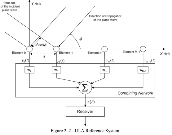
2.3 Reference Antenna System
The antenna array model is composed of M sensors placed at the positions ˆ ˆ ˆ, 0,..., -1
m=xm +ym +zm m= M
p x y z
The reference coordinate system we refer to is scratched in Figure 2. 1. The array sensors are assumes to be isotropic and identical to each other. Consider a narrow band plane wave that impinges on the array from the direction ( , )
θ ϕ
, where θ and ϕ indicate the azimuth and elevation angle, respectively. In the following the angle pair ( , )θ ϕ is called Angle of Arrival (AOA) or Direction of Arrival (DOA) of the plane wave. The assumption of a plane wave holds when the signal source is in the far field of the receive antenna which implies that the radius of the wave front is much bigger than15
Figure 2. 1 - Coordinate System
θ φ
x
yz
ˆβthe physical size of the antenna array. We indicate the phase propagation factor of a wave at the wavelength λ with β
(
)
2 2 ˆ
ˆ ˆ ˆ
cos sin sin sin cos
π φ θ φ θ θ π
λ λ
= − + + =
β x y z β
where ˆβ denotes a unity vector in the direction of propagation of the plane wave. As said our analysis is 2-D and the DOA of the plane wave lies in the azimuth plane
(
π
2,φ
)
. Thus, the phase propagation factor simplifies(
)
2 ˆ ˆ cos sin π φ φ λ = − + β x yThe appearance of the elevation angle θ in the formulas that follow is to be interpreted as an intended reminder that the concepts we come across are true in the volumetric space in general. The phase difference between the received signals at the m-th element of the array and the origin of the coordinate system (x= = = ) is y z 0
m m
ψ
∆ = − ⋅β p
with ⋅ that indicates inner product. Accordingly, the propagation time of the wave to propagate from the array element m to the origin of the coordinate system is ˆ m m c τ = −β p⋅
16 2.4 Narrow Band Antenna Model
In this work we are interested in studying the use of the antenna arrays in telecommunications systems. Thus, We point out the fundamentals of the array processing theory for digital communications applications. In the following we explain the narrow band antenna model in depth. It models the signal reception of narrow band digital information signals by antenna arrays. The reference quantity of the digital signal is the signalling interval which is to be compared with the propagation time that the wave front of the plane wave takes to propagate over the inter element spacing of the array system. If one can assume that the signalling interval of narrow band digital signal is much larger than the characteristic propagation time, thus, at any time epoch t all the sensors in the array system receive the same symbol time. Moreover, the signals captured by the array sensors have the same amplitude but different phases. These phases are the only quantities of the received signal that contain the information of the direction of arrival. Then, direction of arrival estimation can be carried out by manipulating the signal phases at the array sensors output. This concept is formulated in detail in the subsequent sections for the two spatial distributions of array sensors that we have study in this work, that is ULA and UCA.
2.5 Uniform Linear Array Model
The antenna elements of ULA systems are positioned along a linear direction, which is the axis x in our study, with a uniform element spacing
d, Figure 2. 2. The m-th element location is
ˆ ˆ 0,..., -1
m =xm =md m= M
p x x
We indicate with ( )r t the analytic narrow band impinging signal at the origin of the coordinate system. ( )r t is referred to as the reference signal impinging on the array system throughout this document. Its general expression is
17
Figure 2. 2 - ULA Reference System
Σ
( ) z t 0( ) y t y t1( ) y tm( ) yM−1( )t d cos d φ φ 2 ( ) ( ) j f tc r t =µ t e π (2.3)where f is the carrier frequency and ( )c µ t is a narrow band signal bearing the data modulation signal. The m-th array element produces the signal
2 ( ) (2 )
( ) ( ) ( ) j f tc m ( ) j f tc m
m m m m
r t ≜r t+
τ
=µ
t+τ
e π +τ =µ
t+τ
e π +∆ψwhere m represents the element index in the array m=0,...,M -1. In the remainder of this work, the range of m will be omitted.
If the impinging complex modulation signal µ( )t does not vary significantly over
{ }
( 1)max m d M
c
18
which is the propagation time from one sensor to the opposite end-sensor of a plane wave impinging from φ = ° or 0 φ =180° , the simplification
(t m) ( )t
µ +τ ≃µ
holds for all the array elements. For a data-modulated signal this means that
{ }
max
τ
m ≪Twhere T is the signal interval of a data symbol.
Under this condition, the signal captured by the antenna element m differs from the reference signal ( )r t by a phase offset only
(2 )
( ) ( ) j f tc m ( ) j m
m
r t ≃
µ
t e π +∆ψ =r t e ∆ψ (2.4)Indicating with ψo the phase of narrow band incident signal at the origin of the coordinate system, the signal phase at the output of the m-th array branch is 2 cos m o m o m o md o m π ψ ψ ψ ψ ψ φ ψ ψ λ = + ∆ = − ⋅β p = + = + ∆
The phase offset ∆ =ψ βdcosφ between the signals of two adjacent sensors is called the electrical angle and contains the DOA information. We define the vector of the received signals by the array elements as
0 1 2 1
( )t =[y t y t( ), ( ),...,ym( ),...,t yM− ( ),t yM− ( )]t T y
whose m-th entry can be expressed as
( ) ( ) j m ( ) ( ) jm ( )
m m m
y t =r t e− ⋅β r +n t =r t e ∆ψ +n t
( ) m
n t is the noise captured at the array element m and is a complex sample function from an analytic white Gaussian noise process with power spectral density 2N around 0 fc (see Appendix A). By introducing the steering vector or array manyfold of uniform linear arrays of isotropic sensors
( ) ULA φ a ( 1) ( ) [1, j ,..., j M ]T ULA e e ψ ψ
φ
= ∆ − ∆ a (2.5)and defining the noise vector ( )n t as
0 1 2 1
( )t =[n t n t( ), ( ),...,nM− ( ),t nM−( )]t T n
19
{
( ) ( )}
2 0 ( ) H E t u N δ t u = = − n R n n Ithe vector y( )t of the signals captured at the array sensors can be conveniently rearranged as
( )t =r t( ) ULA( )φ + ( )t
y a n
(2.6) The vector notation (2.6) will be used late when we will deal with the DOA estimation. From (2.6), one sees that the noiseless signal at the array output
( ) z t is 1 1 cos 0 0 ( ) ( ) ( ) ( ) ( , ) M M jm d m m m m m z t w y t r t w e β φ r t f θ φ − − = = =
∑
=∑
= (2.7)The factor f
(
θ φ
,)
is termed array factor. It represents the ratio of the received signal which is available at the array output, ( )z t , to the signal input ( )r t , measured at the reference element of the array, as a function of the DOA(
θ φ
,)
. f(
θ φ
,)
is lied to the steering vector aULA( , )θ φ as(
,)
T ULA( , )f θ φ =w ⋅a θ φ (2.8)
where w is the vector of the weighting coefficients
[
0,..., ,..., 1]
T m M w w w − = wFrom (2.8) it is evident that by adjusting the set of weights
{ }
wm it is possible to direct the maximum of the main beam of the antenna factor in any desired direction(
θ φ
0, 0)
. This is the basic mechanism on which to design antenna controllers that performs beamsteering by exploiting the estimates of the DOA of the received signal. This is the approach that we have followed in this work and that will be explained later with more details.2.5.1 Array Factor of ULA Systems
From the analysis of the array factor one can understand the directional properties of the antenna arrays. The parameters of interest are the number of antenna elements in the array M and the inter-element spacing d. We
20
rearrange the expression of the array factor given in (2.8) for the case of unity weighting coefficients as
(
)
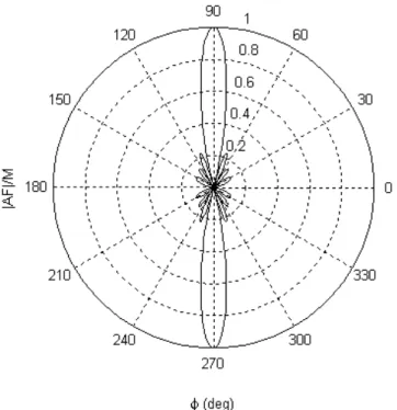
1 cos 2 cos sin 2 , cos sin 2 M j d M d f e d β φ β φ θ φ β φ − = (2.9)In Figure 2. 3a and 1.3b, we have plotted the amplitude of the array factor (2.9) normalised to M, for different values of M. It is evident that increasing M determines the following effects on the radiation patterns:
• The width of the main lobe of the radiation pattern reduces. This is crucial for applications where smart antennas are employed to track a mobile device with a single narrow beam. This point will be highlighted later when analysing the system requirements of the antenna controller.
• The number of sidelobes increases. At the same time, the level of the sidelobes decreases compared with the one of the main lobe. Sidelobes are important in wireless systems communication since they represent radiated or received power, in unwanted directions. • The number of nulls in the patter increases. In interference
cancellation applications, the directions of those nulls as well as the null depth has to be optimized.
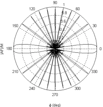
The inter element spacing d also has a significant impact on the shape of the radiation pattern. It is known that the directional properties of the antenna array depend on the array size. Increasing the array size by increasing the number of sensors M gets better characteristics of the radiation pattern as far as its shape and degrees of freedom. But, the array size can be increased also by increasing the inter-element separation d. By playing on d we can customize the design of antenna arrays. The main observation that we draw when analysing the normalized array factor versus d is the appearance of replicas of the main beam which are names gratings lobes. In Figures 2.4 we have plotted the array pattern of a 8-element antenna array for different
21
Figure 2. 3a - Radiation Pattern of ULA Systems with d=λ/2
-50 -40 -30 -20 -10 0 |A F | (d B ) 150 120 90 60 30 0 φ (deg) M=4 M=8
values of d. As is seen when d is
λ
4orλ
2, Figure 2. 4a and Figure 2. 4b respectively, the array pattern is composed of one main lobe at 90° and a few sidelobes. The main lobe of the array pattern is termed boresight. When d isλ, Figure 2. 4c, a grating lobe appears at 0°. When d becomes greater than λ more grating lobes appear as shown in Figure 2. 4d. To see this, consider that from (2.9), the maxima of the array factor are the solutions in the φ of the equationcos sin 0 2 d β φ = which gives cos d λ φ =
22
Figure 2. 4a - Polar Radiation Pattern of ULA Systems with d=λ/4 Figure 2.3b - Radiation Pattern of ULA Systems with d=λ/2
-50 -40 -30 -20 -10 0 | A F | (d B ) 150 120 90 60 30 0 φ (deg) M=12 M=16
23
Figure 2.4c - Polar Radiation Pattern of ULA Systems with d=λ Figure 2.4b - Polar Radiation Pattern of ULA Systems with d=λ/2
24
Figure 2.4d - Radiation Pattern of ULA Systems with d=5λ
Notice that the grating lobes differ from the sidelobes because they have the same magnitude of the gain as the main lobes. Thus in applications where we intend to apply transmit diversity to combat the fading effects we can intentionally use antenna arrays designed with d up to 10λ to exploit the angle spread of the fading. In applications where the aim is the array directivity only, grating lobes are very difficult to deal with since they produce a significant waste of power emitted in unintended directions and more interference captured than the sidelobes. As a general rule, in this class of applications, d is chosen to be less than λ but more than
λ
2 to limit the mutual coupling effects among the sensors. In practice,λ
2is the usual inter-element distance and an array having the elements spaced ofλ
2 is said standard array. In the following we will refer to standard arrays unless otherwise specified.25
Figure 2. 5 – 8-element UCA Reference System
x
R
2 M πy
d2.6 Uniform Circular Antenna Model
Uniform Circular Array systems are composed of sensors which are disposed along a ring with a uniform angle separation of 2
π
M , Figure 2. 5. The m-th sensor position isˆ ˆ
(cos sin )
m =R φm + φm
p x y
where R is the radius of the circle and φm is the azimuth angle of the m-th sensor 2 m m M π φ =
With d that indicates the inter element distance, the relationship between R, M and d is 2 2 1 cos d R M
π
= − (2.10)As with ULA systems, indicating with ( )r t the analytic narrow band incident signal at the origin of the coordinate system and with
ψ
oits phase, if it is possible to assume that( ) ( m)
r t ≃ r t−
τ
∀m26
{ }
2max m R
c
τ
=the noisy signal available at the output of the m-th array element can be written as ( ) ( ) j m ( ) m m y t =r t e− ⋅β r +n t whose phase is 2
(cos cos sin sin )
m o m o R m m
π
ψ
ψ
ψ
φ
φ
φ
φ
λ
= − ⋅β p = + +
The steering vector of UCA systems can be defined as
( ) ( ) 0 1 cos cos ( ) M j R UCA j R e e β φ φ β φ φ
φ
− − − = a ⋮ (2.11)and the vector ( )y t of the signals available at the array output can be expressed similarly to (2.6)
( )t =r t( ) UCA( )
φ
+ ( )ty a n
2.6.1 Array Factor of UCA Systems
The array factor of ULA systems with unity weighting coefficients is
( ) 1 cos 0 ( , ) m M j R m f
θ φ
e β φ φ − − = =∑
(2.12)The advantage of a circular array is that it creates only one man beam that can be swept fully around the circle. Similar to linear arrays, the number of elements in the array determines the width of the meanbeam and the element spacing determines the entity of the sidelobes. In ULA system the choice of keeping the element spacing lower than half a wavelength is dictated by the appearance of grating lobes. In UCA systems a similar choice is made in order to limit the pattern ripple [26], a possible criterion is to keep below 1 dB. The pattern ripple is measured by the ratio of the maximum array factor to the minimum array factor. The more the pattern ripple the more the array pattern deviates from the omnidirectional radiation when the sensors are fed
27
Figure 2. 6 - Polar Radiation Pattern of a 8 element UCA with kR=5.2
M kR Ripple dB
8 4.10469 0.4 12 6.0691 0.1262 16 8.05164 0.01861
Table 2. 1– Ripple values for the sensor arrangement d=λ 2
with equal phases and amplitudes as seen in Figure 2. 6 for a 8 element array with kR =5.2.
The pattern ripple of the array of Figure 2. 6 amounts to 2 1 10 log 8 0.4 dB ≃
In Table 2. 1 we have reported the calculated ripple by using (2.12) as resulting from the sensor arrangement d =
λ
2.28
As is seen the more M, the less the ripple. For M less than 8 instead, d has to be less than
λ
2. For instance with 4 elements, d =0.35λ gives 0.97 dB ripple.2.7 Antenna Directivity
.
The power density, having units of W/rad2, for a particular direction
(
θ φ
,)
is given by U( , )
θ φ
. It is of practical interest the relationship between the power density U( , )θ φ
and the array factor AF( , )θ φ
so as to derive the antenna directivity from the geometry of the array system. U( , )θ φ
as a function of the array factor AF( , )θ ϕ
is(
)
(
)
2, ,
U
θ φ
= AFθ φ
(2.13)The total power transmitted in all directions is
(
)
2 0 0 , sin rad P π π U d d φ= θ= θ ϕ θ θ φ =∫ ∫
The average power density, Uave, is(
)
2 0 0 1 , sin 4 4 t ave P U π π U d d φ θ θ ϕ θ θ φ π π = = = =∫ ∫
(2.14)When the antenna transmits power equally in all directions, the antenna is said to be isotropic. Isotopic antennas are often used as a reference case. Antenna arrays have the ability to concentrate the radiated power in a particular angular direction in space. This ability is measured by the directive gain defined as
(
,)
(
,)
ave U D U θ φ θ ϕ = (2.15)The directive gain in the direction of the maximum radiation density is referred to as the directivity, D , and is given
(
)
{
}
, max , ave U D U θ φθ φ
=29
(
,)
4(
,)
in U G Pπ
θ φ
θ ϕ
=where P is the total input power to the array. By defining the antenna in efficiency η, which accounts for losses, as
rad in P P
η
= it follows that(
,)
(
,)
Gθ φ
=η
Dθ φ
In our work, the antenna is assumed to be lossless and perfectly matched, so as we will interchangeably refer to the antenna gain or antenna directivity.
2.7.1 Directive Gain of ULA Systems
The directive gain of ULA systems can be found as follows. We first substitute (2.9) in (2.13) to write the power density. We then substitute (2.13) in (2.14) and (2.13)-(2.14) in (2.15). The final expression is
(
)
2 2
2 2 2
0 0
cos sin cos sin
4 sin sin
2 2
,
cos sin cos sin
sin sin sin
2 2 M d d D M d d d d π π
β
φ
θ
β
φ
θ
π
θ φ
β
φ
θ
β
φ
θ
θ θ φ
= ∫ ∫
(2.16) 2.7.2 Directive Gain of UCA SystemsThe derivation of the directive gain of UCA systems is similar to ULA systems with the only difference that (2.9) replaces (2.12). The directive gain is
(
)
( ) ( ) 2 1 sin cos 0 2 1 2 sin cos 0 0 0 4 , sin m m M j R m M j R m e D e d d β θ φ φ π π β θ φ φπ
θ φ
θ θ φ
− − = − − = =∑
∑
∫ ∫
(2.17)30 2.8 Beamsteering
Beamsteering is the simplest form of beamforming. It can be achieved by a delay-and-sum beamformer with all its weights equal in magnitude and the phases selected to steer the antenna boresight in any wanted direction
φ
0 known as the look direction. As an example, this goal can be achieved with these choices of weighting coefficients0 cos 1 j md m w e M β φ − = (2.18) and ( 0 ) cos 1 j R m m w e M β φ φ − − = (2.19)
for ULA and UCA systems respectively.
2.8.1 Beamsteering of ULA Systems
To see the effect of this operation we write the array factor or equivalently the directive gain of ULA systems by introducing the weighting coefficients (2.18) in (2.8). The resulting expression of the array factor is
(
)
( )(
)
(
)
0 0 1 cos cos 2 0 cos cos sin 2 , cos cos sin 2 M j d M d f e d β φ φβ
φ
φ
θ φ
β
φ
φ
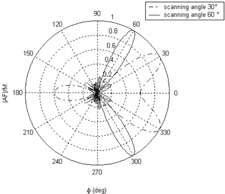
− − − = − (2.20)which is straightforwardly comparable with (2.9). In Figure 2. 7 we have plotted (2.20) for
φ
0 =30° andφ
0 =60° for an 8-element linear-phased standard array. In particular whenφ
0 = ° the array is said end-fire whereas 0 whenφ
0 =90° the array is said broadside. Figure 2. 8 depicts the directive gain of a standard linear-phased array with weighting elements (2.18) in the plane x-y andφ
ranging in [0°,180°), for M equal to 8 (9 dBi), 12 (10.79 dBi) and 16 (12 dBi) and for three values of the scanning angleφ
0, 0°, 45° and 90°, respectively. As said, increasing the number of elements determines a higher antenna directivity and a narrower mainlobe beamwidth. We point out that the reduction of the mainlobe beamwidth due31
to an increasing M has a different importance if analysed versus the pointing direction
φ
0. In fact in general, for a fixed M, the beamwidth of uniform linear antenna arrays is narrower if the array is broadside and becomes broader outwards with the maximum at end-fire. Such a variation is more noticeable with M that increases. It can be observed that an increase of M up to 16 leaves the beamwidth still large ifφ
0 = ° whereas it gives a sharp and 0 narrow mainlobe ifφ
0 =90° . The behaviour of the beamwidth for ULA systems is treated in more details in the next section.The steering process is similar to steering the array mechanically in the look direction, except that it is done electronically by adjusting the phases of the signals at the array elements outputs. This later is also referred to as electronic steering, and phase shifters are used to adjust the phases. The phase offset form one element to the next in ULA systems is
0
cos
π
φ
which amounts to 0° for broadside and to π for end-fire.
If
φ
0 is the AOA of the far field source, we want to point the antenna in the AOA of the impinging signal to receive the signal. Said aULA( )φ
0 the steering vector of the ULA system in the AOA of the impinging source, the weighting coefficients vector (2.18) is0 1 ( ) ULA M
φ
∗ = w aThe array with these weights has unity response in the look direction, that is, the mean output power of the processor due to a source in the look direction is the same as source power. Assume that the data modulation signal ( )
µ
t in (2.3) has mean power pµ, from (2.7) one gets the mean output power( ) H( ) ( ) P w =E z t ⋅z t = pµ
Thus, the mean output power of the beamformer steered in the look direction is equal to the power of the signal in the look direction. In the special case where the system is dominated by uncorrelated noise, 2
n
σ
=
n
R I ,
and no interference exists in the look direction, this beamformer provides maximum SNR. In fact, the noise output power is
32 16 14 12 10 8 6 4 2 0 S ta n d a rd U L A D ir e c ti v e G a in ( 9 0 °, φ ) 180 160 140 120 100 80 60 40 20 0 φ deg M=8 M=12 M=16
Figure 2. 8 - Standard ULA Directive Gain, φ0=0°, 45°, 90° Figure 2. 7 - Beamsteered 8-element standard ULA System
33 2 T n M
σ
= = n n P w R wThe processor with unity gain in the direction of the source has reduced the uncorrelated noise by a factor M, yielding an output SNR
2 out n p SNR M µ
σ
= when the input SNR is2 in n p SNR µ
σ
=This beamformer provides an array gain, which is defined as the ratio of the output SNR to the input SNR, equal to the number of elements in the array M.
This beamformer requires some prior knowledge about the look direction
φ
0 to be applied. In this work we study the CRB for DOA estimation and the impact of the accuracy of those estimates onto the goodput performance of phased array controllers that use DOA estimates for beamsteering.2.8.2 Beamsteering of UCA Systems
In this section we analyse the normalized array factor of UCA systems with the substitution of (2.19) in (2.12) for beamsteering with an inter element separation of half a wavelength. Figure 2. 9a refers to a 8-element array pointing two directions,
φ
0 =45° andφ
0 =22° , respectively. We have also plotted the case of a 12-element array to show the increase in directivity due to more elements in the array, Figure 2. 9b. For the 8 element array we note the presence of a relevant back lobe compared to the 8-element standard linear array of Figure 2. 7. As said UCA systems can scan all the azimuth circle with only one beam. However we note that the relative direction of the beam compared to the location of the sensors can cause a nonsymmetric pattern and the appearance of some relatively large sidelobe. For instance, in Figure 2. 9a one notices that the sidelobe at 150° of the array pattern when0 45
34
Figure 2. 9b - 12-element UCA System steered at 45° Figure 2. 9a - 8-element UCA System steered at 45°
35 50 40 30 20 10 H P B W ( d e g ) 2.0 1.5 1.0 0.5 d/λ M=4 M=8 M=12 M=16
Figure 2. 10a - Beamwidth of ULA systems as a function of d/λ
2.9 Half Power Beamwidth of ULA Systems
The half-power beamwidth (HPBW) or simply beamwidth is defined as: “In a plane containing the direction of the maximum of a beam, the angle between the two directions in which the radiation intensity is one-half the maximum value of the beam”. Thus the term beamwidth is implicitly reserved to indicate -3dB beamwidth. An important indication provided by the beamwidth if the resolution capacity of the antenna that is the capacity of the antenna to distinguish between to sources. Two sources separated by angular distances equal or greater than HPBW can be resolved [27].
A general formula for the beamwidth of a linear-phased array is [28]
1 1
cos cos o 0.443 cos cos o 0.443
HPBW Md Md
λ
λ
φ
φ
− − = − − + (2.21)which is valid for a wide range of scanning angles but not for end-fire. In Figures 2.10a and 2.10b we notice the same behaviour for the beamwidth when we increase d and M. Figure 2.10c demonstrates that the beamwidth of a linear-phased array of a given size is not constant but rather it depends on the scanning angle.
36 50 40 30 20 10 H P B W ( d e g ) 16 14 12 10 8 6 4 M d=0.25λ d=0.5λ d=0.75λ d=λ
Figure 2.10b - Beamwidth of ULA systems as a function of M
40 30 20 10 H P B W ( d e g ) 90 80 70 60 50 40 φ (deg) M=4 M=8 M=12 M=16
37
Chapter III. Simulation Analysis with IEEE
802.15.3c MAC
3.1 General Description of IEEE 802.15.3
In this section we provide a brief description of the IEEE 802.15.3 standard. In that, we have picked up those features of the standard that serve to set the background for the explanation of the design of the IEEE 802.13.3 phased array controller throughput, which is our aim in this chapter.
A piconet is a wireless ad hoc data communication system which allows a number of devices (DEVs) to communicate with each other. A piconet differs from other data networks in that communications are confined to a limited area around a person or an object. The target radio coverage of the mm-wave WPANs goes from desktop and body applications to the in-room like applications. A 802.15.3-based piconet consists of several components. The main are shown inFigure 3. 1. One DEV is required to assume the role of the coordinator of the piconet (PNC). It provides the basic timing for the piconet with the beacon. Additionally, the PNC manages the QoS requirements, power saving modes, and access control to the piconet. Because 802.15.3 networks form without pre-planning and only for as long as the piconet is needed, this type of operation is classified as an ad hoc network. 802.15.3 specifies allocation of a subsidiary piconet generally referred to as dependent piconet. In our work we have neglected allocation of dependent piconets.
Timing in the 802.15.3 piconet is based on the superframe, which is illustrated in Figure 3. 2. The superframe is composed of three parts:
• The beacon is used to set the time timing allocations and to communicate management information for the piconet.
38
Figure 3. 2 - Superframe composition Figure 3. 1 - Piconet components DEV DEV DEV DEV PNC/ DEV data data data data data beacon beacon bea con beacon
• The contention access period (CAP) is used to communicate commands and/or asynchronous data if it present in the superframe. • The channel allocation period (CTAP) is composed of channel time
allocations (CTAs), including management CTAs (MCTAs). CTAs are used for commands, isochronous streams and asynchronous data connections.
The CAP uses CSMA/CA for the medium access. The CTAP uses a standard TDMA protocol where the DEVs have specified time windows. MCTAs are either assigned to a specific source /destination pair and use TDMA for medium access or shared CTA that use slotted aloha protocol. In this work MCTAs are neglected.
39
There three methods for communicating data among DEVs in a piconet: 1) Sending asynchronous data in the CAP, if present. DEVs can send small
amounts of data without having to allocate channel time.
2) Allocating channel time for isochronous streams in the CTAP. This kind of communication is requested by a DEV that needs time allocation on a regular basis. If the resources are available the PNC reserves a CTA for the DEV. The isochronous CTAs can be either static or pseudo-static. If a DEV misses a beacon, the DEV cannot use the CTA in the next superframe if the CTA is of the first type. If the CTA request is of the second type, the device can still use the CTA in the subsequent superframe up to a mMaxLostBeacons of missed beacons.
3) Allocating asynchronous channel time in the CTAP. Unlike isochronous allocation, it corresponds to a request for a total amount of time needed to transfer a given bulk of data. The PNC schedules channel time for this communication according to the current channel time requests.
In this work, we have taken into consideration isochronous communications only, and pseudo-static CTAs only.
To verify the delivery of frame the standard specifies three types of ACKs to enable different applications.
1) The no-ACK policy is appropriate for frames that do not require guaranteed delivery where the retransmitted frame would arrive too late or where an upper layer protocol is handling a the ACK and the retransmission.
2) The Immediate-ACK (Imm-ACK) policy is an ACK process in which each frame is individually acknowledged after the reception of the frame. 3) With the Delayed-ACK (Del-ACK) frames are acknowledged in groups.
The ACK is sent when requested by the source DEV. This ACK policies decreases the overhead with respect to the Imm-ACK while ensuring t the source DEV the verification of a successful transmission.
40
Table 3. 1- MAC related System Attributes
As seen, the MAC mechanisms included in this standard make it sufficiently flexible to operate with a wide range of wireless applications having different QoS requirements, bandwidth demands and traffic types. Table 3. 1Errore. L'origine riferimento non è stata trovata. shows how this MAC standard fits the wireless applications that are envisaged to be operative in the 60 GHz band.
# Application MAC Related Systems Attributes 1
Uncompressed HDTV Video/Audio streaming [DVD players and other power-line operated
devices]
a) Isochronous
b) High throughput efficiency c) Point-to-Point
d) Support for high gain antennas for Data Transmission e) Device discovery
f) Moderate latency
g) Minimum reserved bandwidth 2
HDTV Video/Audio streaming [video camera/mobile devices
and other battery operated devices]
a) Isochronous
b) High throughput efficiency
c) Maintain link throughput while in motion jitter d) Point-to-Point
e) Support for moderate gain antennas for Data Transmission f) Automatic device discovery
g) Moderate latency
h) Minimum reserved bandwidth i) Multiple nearby data transmissions 3
Internet bulky music and video downloading [computing devices]
a) Asynchronous
b) High throughput efficiency c) Point-to-Point
d) Support for moderate gain antennas for Data Transmission e) Device discovery (Automatic preferred)
4
Internet bulky music and video downloading
[mobile devices]
a) Asynchronous
b) High throughput efficiency c) Point-to-Point
d) Support for moderate gain antennas for Data Transmission e) Device discovery (Automatic preferred)
f) Multiple nearby data transmissions g) Power saving mode
5
Internet small size file transfer (email, web,
chat)
a) Asynchronous b) Point-to-Point
c) Support for moderate gain antennas for Data Transmission d) Device discovery (Automatic preferred)
e) Multiple nearby data transmissions f) Power saving mode
g) Fast connect 6
Local file transfer for printing, document and
small size file
a) Asynchronous b) Point-to-Point
c) Support for moderate gain antennas for Data Transmission d) Device discovery (Automatic preferred)
e) Multiple nearby data transmissions f) Power saving mode
41 7 Local file transfer for
bulky music and video, point-to-point connection
(photo/video camera and photo/video handy phone, mp3 player)
a) Asynchronous b) Point-to-Point
c) Support for moderate gain antennas for Data Transmission d) Device discovery (Automatic preferred)
e) Multiple nearby data transmissions f) Power saving mode
8
Wireless docking station
a) Isochronous
b) High throughput efficiency
c) Maintain link throughput while in motion jitter d) Point-to-Point
e) Support for moderate gain antennas for Data Transmission f) Device discovery (Automatic preferred)
g) Moderate latency
h) Minimum reserved bandwidth i) Multiple nearby data transmissions 9
Video supply, Environment bus, train,
airplane
a) Isochronous
b) High throughput efficiency
c) Broadcast, multicast and unicast capable d) Minimum reserved bandwidth e) QoS support
f) Low delay jitter (<100 ms) g) Moderate latency (< 100 ms)
h) Support of asymmetric data rates and gaming
i) Cumulative acknowledgements and unacknowledged streaming j) Infrastructure mode (non ad-hoc)
k) Secondary (fallback) PHY for 100% coverage and uplink
3.2 Adapting IEEE 802.15.3c MAC for the Use of Phased Array Antennas In this section we describe the extension of the IEEE 802.15.3 MAC for the use of phased array antennas. The array system does include the omni directional operating mode. Omni operations are directly involved into this directional protocol and ensure compatibility with devices that are not equipped with array antennas. For this reason, our protocol can be thought as an extension to the PHY-MAC functionalities of IEEE 802.15.3c when directional antennas are used. In the following we first explain the basic mechanism of our neighbour discovery protocol which is based on DOA estimation of the incoming frames. We then illustrate how this mechanism is employed to establish both PNC-DEV and DEV-DEV wireless links.
3.2.1 DOA Estimation on the PHY Preamble
In this section we show a revisited modelling approach first proposed in [29] for directional antenna adaptation. Figure 3. 3 shows the timeline of a
42
Figure 3. 3 - Data frame exploitation for antenna adaptation
received frame. It composes of a PHY part and a MAC part. DOA estimation can be carried out on the preamble of the PHY of the received frame. The physical preamble is assumed to be a known OFDM long training sequence added to aid receiver algorithms of synchronization, carrier-offset recovery and channel equalization. In particular, as far as the DOA estimation is concerned, we simplify the modelling of a training sequences as one OFDM symbol having both the number and the positions of the pilot subcarriers known. DOA estimation is accomplished in the PHY preamble time Tpp and the DOA estimate is used to point the main beam in
the direction of arrival of the frame during the remainder of the frame receive time Tframe - Tpp. If frame reception is successful, the DOA estimate
is cached and the DEV switches to the narrow beam communication. The DEV can use the DOA just acquired either to reply to the sending DEV directionally or as the expected DOA of the next frame from the same source. In this second case then, the next frame is received with a receive antenna already beam steered to the DOA of the frame.
It should be noted that:
1) DOA estimation with no DOA information cached occurs during the Tpp.
of the first frame of a wireless communication or after a protocol reset, for instance due to the loss of the direction toward the intended DEV. With reference to Figure 2. 2, DOA estimation in these conditions is actually performed on the signals vector y at the output of the array sensors, before the multiplication by the weighting elements w.
2) DOA estimation performed with a receive antenna already pointed benefits from a maximum SNR as explained in Section 1.9.1. In this
43
case the signals vector used for estimation is z at the output of the array sensors after the multiplication by the weighting elements w.
3) DOA estimation could be carried out, let us say refreshed or refined, during the symbol times composing Tframe - Tpp. Concentrating the
estimation in Tpp can be thought as representative of the performance
estimation achievable on whatever number of symbols in the interval Tframe.
3.2.2 Frame Driven Beamsteering in IEEE 802.15.3c MAC
In a piconet there are two kinds of wireless links. One is the PNC-DEV link, The other id the DEV-DEV link.
• Antenna steering on beacon time. All the DEVs set their local timing information upon receiving the beacon. Beacon reception serves as a time reference for clock synchronization in the network. Beacon transmission is intrinsically broadcast to keep the differences of the instants at which the beacon is received at the DEVs within the guard intervals fixed by the standard and avoid time differences due to the protocol. The wireless link PNC-DEVs as far as the beacon transmission is concern is omni at the PNC and can be directional at the DEVs. That is, the PNC-DEVs links antenna gain is exploited at the receiver only. To overcome the link gain asymmetry, the MAC beacons are transmitted at a lower rate. The lower rate transmission rate results in a lower SNR requirement that with less antenna gain in the link should end up with the same probability of correct frame reception. This mechanism represents a form of MAC-PHY cross-layer optimization that can be implemented with the addition of a few PHY-SAP (Service Access Point) primitives. For instance consider the current IEEE 802.15.3 PHY specification. To achieve FER ≤8%with a transmission rate of 55 Mb/s and 64-QAM-TCM, we need