The AGN-Star Formation Connection: Future Prospects with JWST

2021-02-08T15:18:42Z

Acceptance in OA@INAF

The AGN-Star Formation Connection: Future Prospects with JWST

Title

Kirkpatrick, Allison; Alberts, Stacey; Pope, Alexandra; Barro, Guillermo; BONATO,

MATTEO; et al.

Authors

10.3847/1538-4357/aa911d

DOI

http://hdl.handle.net/20.500.12386/30243

Handle

THE ASTROPHYSICAL JOURNAL

Journal

849

The AGN

–Star Formation Connection: Future Prospects with JWST

Allison Kirkpatrick1 , Stacey Alberts2, Alexandra Pope3 , Guillermo Barro4 , Matteo Bonato5, Dale D. Kocevski6, Pablo Pérez-González7, George H. Rieke2 , Lucia Rodríguez-Muñoz8 , Anna Sajina9 , Norman A. Grogin10 ,

Kameswara Bharadwaj Mantha11, Viraj Pandya12 , Janine Pforr13, Mara Salvato14 , and Paola Santini15

1

Yale Center for Astronomy & Astrophysics, Physics Department, P.O. Box 208120, New Haven, CT 06520, USA;allison.kirkpatrick@yale.edu

2

Steward Observatory, University of Arizona, 933 North Cherry Avenue, Tucson, AZ 85721, USA

3

Department of Astronomy, University of Massachusetts, Amherst, MA 01002, USA

4_{University of California, 501 Campbell Hall, Berkeley, CA 94720 Santa Cruz, USA} 5

INAF—Osservatorio di Radioastronomia, Via Piero Gobetti 101, I-40129 Bologna, Italy

6

Department of Physics and Astronomy, Colby College, Waterville, ME 04901, USA

7

Departamento de Astrofísica y CC. de la Atmósfera, Universidad Complutense de Madrid, E-28040 Madrid, Spain

8

Dipartimento di Fisica e Astronomia, Università di Padova, vicolo dellOsservatorio 2, I-35122 Padova, Italy

9

Department of Physics & Astronomy, Tufts University, Medford, MA 02155, USA

10

Space Telescope Science Institute, 3700 San Martin Drive, Baltimore, MD 21218, USA

11_{Department of Physics and Astronomy, University of Missouri–Kansas City, 5110 Rockhill Road, Kansas City, MO 64110, USA} 12

UCO/Lick Observatory, Department of Astronomy and Astrophysics, University of California, Santa Cruz, CA 95064, USA

13_{ESA/ESTEC, Keplerlaan 1, 2201 AZ Noordwijk, The Netherlands} 14

Max Planck Institut für Extraterrestrische Physik, Giessenbachstraße, D-85748 Garching, Germany

15_{INAF—Osservatorio Astronomico di Roma, via di Frascati 33, I-00078 Monte Porzio Catone, Italy}

Received 2017 June 26; revised 2017 September 14; accepted 2017 September 28; published 2017 November 7 Abstract

The bulk of the stellar growth over cosmic time is dominated by IR-luminous galaxies at cosmic noon( = –z 1 2),

many of which harbor a hidden active galactic nucleus(AGN). We use state-of-the-art infrared color diagnostics, combining Spitzer and Herschel observations, to separate dust-obscured AGNs from dusty star-forming galaxies (SFGs) in the CANDELS and COSMOS surveys. We calculate 24 μm counts of SFGs, AGN/star-forming “Composites,” and AGNs. AGNs and Composites dominate the counts above 0.8 mJy at 24 μm, and Composites form at least 25% of an IR sample even to faint detection limits. We develop methods to use the Mid-Infrared Instrument (MIRI) on JWST to identify dust-obscured AGNs and Composite galaxies from ~ –z 1 2. With the sensitivity and spacing of MIRIfilters, we will detect >4 times as many AGN hosts as with Spitzer/IRAC criteria. Any star formation rates based on the 7.7μm PAH feature (likely to be applied to MIRI photometry) must be corrected for the contribution of the AGN, or the star formation rate will be overestimated by ∼35% for cases where the AGN provides half the IR luminosity and ∼50% when the AGN accounts for 90% of the luminosity. Finally, we demonstrate that our MIRI color technique can select AGNs with an Eddington ratio of lEdd~ 0.01 and will identify AGN hosts with a higher specific star formation rate than X-ray techniques alone. JWST/MIRI will enable critical steps forward in identifying and understanding dust-obscured AGNs and the link to their host galaxies.

Key words: galaxies: active – galaxies: photometry – galaxies: star formation 1. Introduction

The galaxies most actively contributing to the buildup of stellar mass at cosmic noon( ~ –z 1 2) contain large amounts of

dust(e.g., Murphy et al.2011; Madau & Dickinson2014, and references therein). This dust obscures the majority of star formation, making it necessary to study these galaxies through their dust emission at infrared wavelengths (Madau & Dickinson 2014). Additionally, the majority of supermassive

black hole growth at these redshifts is also heavily dust obscured (e.g., Hickox & Markevitch 2007). Many of the

massive dusty galaxies contain a true mix of star formation and obscured black hole growth, the obscured signatures of which can be seen in their infrared spectral energy distribution(SED). These galaxies are then ideal laboratories for understanding the physical link between star formation and active galactic nuclei (AGNs). The AGN–star formation connection is an open question, particularly whether AGN feedback is a key component of star formation quenching, and whether all galaxies have a distinct star formation phase followed by an AGN phase before ultimately quenching (e.g., Sanders et al.

1998; Hopkins et al. 2006). The nature of AGNs within

strongly star-forming galaxies(SFGs) (what we term “Compo-sites”) is even more uncertain. Do these objects represent a unique phase between SFGs and AGNs? Unfortunately, due to limitations of previous space telescopes, detailed studies of the energetics of these objects were severely restricted, but the James Webb Space Telescope (JWST) will reveal their true nature.

Prior to JWST, the most reliable method for identifying Composites and disentangling AGN emission from star formation was with mid-IR spectroscopy, particularly from the IRS instrument on board the Spitzer Space Telescope. The low-resolution spectra can be modeled as a combination of star formation features (most notably the polycyclic aromatic hydrocarbons [PAHs] that exist in photodissociation regions and in stellar/HII regions) and hot continuum emission primarily arising from a dusty torus surrounding the accreting black hole(Pope et al. 2008; Coppin et al. 2010; Kirkpatrick et al. 2012; Sajina & Yan et al. 2012; Hernán-Caballero et al.2015; Kirkpatrick et al.2015). In this way, the division of

IR luminosity between star formation and an AGN can be quantified. The medium-resolution spectrometer (Wells

et al. 2015), which is part of the Mid-Infrared Instrument

(MIRI) on JWST, will enable separation of PAH emission from continuum in the same manner, but with higher resolution and on smaller spatial scales within host galaxies. It will also enable detection of high-ionization gas lines excited by the AGN (Bonato et al.2017), further improving our ability to detect and

measure the physical properties (such as accretion rates and Eddington ratios) of dust-obscured black holes.

As there are only a few hundred Spitzer IRS spectra available for distant galaxies (Kirkpatrick et al.2015), color techniques

were also developed to identify large samples of luminous dust-obscured AGNs. The most popular color selection techniques are with Spitzer IRAC photometry (Lacy et al. 2004; Stern et al. 2005; Alonso-Herrero et al. 2006; Donley et al. 2012),

which separates AGNs using different combinations of the 3.6, 4.5, 5.8, and 8.0μm filters. The original techniques presented in Lacy et al.(2004) and Stern et al. (2005) were limited to the

most luminous AGNs and become increasingly contaminated with galaxies when deeper IR data are used (Mendez et al. 2013). Moreover, with increasing redshift, the rest

wavelengths of these bands decrease, causing contamination of the AGN signatures by SFGs to become significant such that the original IRAC-based criteria cannot be applied. Donley et al. (2012) propose more conservative IRAC criteria that, at

cosmic noon, essentially separate galaxies that exhibit a so-called stellar bump(emission from stars that peaks at ∼1.6 μm and then declines to a minimum around∼5 μm) from those that do not, where the torus radiation is strong enough tofill in the dip in the star-forming spectrum around 3–5 μm, producing power-law emission such as is typical of unobscured AGNs (e.g., Elvis et al. 1994). The Donley et al. (2012) criteria

increase the reliability of AGN color selection, although they are less complete owing to excluding Composites, where the IR emission of the AGN does not dominate over the star formation.

For the purposes of probing the AGN–star formation connection, the limitation of IRAC techniques is that AGNs within strongly SFGs can have different levels of host contamination. Then, many galaxies containing AGN signa-tures at longer wavelengths will also include a stellar bump and therefore be missed(Kirkpatrick et al.2013,2015). To alleviate

host contamination, Messias et al.(2012) propose combining K

band with IRAC and 24μm to separate AGNs from host galaxies all the way out toz~7. Going further, including mid-IR and far-mid-IR (Fmid-IR) colors can greatly improve the selection of Composite galaxies, since this will trace the contribution of warmer AGN-heated dust compared with cold dust from the diffuse interstellar medium in the host galaxy (Kirkpatrick et al. 2015). However, this requires observations from the

Herschel Space Observatory, which have a large beam size and do not reach the same depths as Spitzer observations. Perhaps the most reliable method is fitting a full suite of photometry from the UV to the FIR. This is an emergent technique that can also be used to quantify the fraction of bolometric luminosity due to an AGN (e.g., Calistro Rivera et al. 2016). MIRI

photometry can be combined with NIRcam and Hubble Space Telescope photometry to simultaneously quantify the stellar population, dust obscuration, and AGN energetics. The draw-back to this technique is that it requires a careful merger of photometry from different instruments and measured in different ways. It also is more sensitive to degeneracy in the

solution and assumes a good understanding of the templates used in thefit.

MIRI will greatly improve color selection techniques owing to the increased sensitivity and the number of transmission filters covering the mid-infrared (Bouchet et al.2015; Glasse et al.2015). Now, we will be able to separate AGNs from SFGs

by comparing PAH emission with the minimum emission from stars that occurs around 5μm; in AGNs, the stellar minimum is not visible owing to strong torus emission, and Composites will lie in between strong AGNs and pure SFGs in color space.

In this paper, we build on the Herschel and Spitzer color selection techniques initially presented in Kirkpatrick et al. (2013) to identify Composite galaxies at ~ –z 1 2 using the CANDELS(0.24 deg2) and the entire COSMOS (2 deg2) fields. We present galaxy counts of 24μm sources classified as SFGs, AGNs, or Composites based on their IR colors, making this the first identified statistical sample of Composites at cosmic noon. We use this sample to predict black hole and star formation properties of samples that JWST/MIRI will identify. We also present color diagnostics for identifying both AGNs and Composites using JWST/MIRI filters in three redshift bins. Throughout this paper, we assume a standard cosmology with

= -

-H0 70 km s 1Mpc 1, WM = 0.3, and W =L 0.7. 2. CANDELS and COSMOS Catalogs

To calculate galaxy counts, we use Spitzer and Herschel photometry from the COSMOS, EGS, GOODS-S, and UDS fields from the Cosmic Assembly Near-IR Deep Extragalactic Survey(CANDELS, P.I. S. Faber and H. Ferguson; GOODS-Herschel, P.I. D. Elbaz; CANDELS-GOODS-Herschel, P.I. M. Dick-inson). We do not include GOODS-N, as, at the time of the writing of this paper, the IR catalog does not have uniquely identified optical counterparts. We also use photometric redshifts(z ;phot Dahlen et al.2013; Stefanon et al. 2017) and M_* (Santini et al. 2015; Stefanon et al. 2017). The stellar

masses are derived by fitting the CANDELS UV/Optical photometry in 10 different ways, eachfit using a different code, priors, grid sampling, and star formation histories(SFHs). The final M_*is the median from the different fits, and it is stable against the choice of SFH and the range of metallicity, extinction, and age parameter grid sampling. The CANDELS

zphotsare the median redshift determined throughfive separate codes that fit templates to the UV/optical/near-IR data (the technique is fully described in Dahlen et al.2013). Comparison

of zphotswith spectroscopic redshifts for a limited sample gives

s = 0.03, where σ is the rms of(zphot-zspec) (1 +zspec). As we sort sources into redshift bins of D =z 0.5, we do not expect the uncertainty on the photometric redshifts to be a dominant source of uncertainty in our results. We will be using the zphots to help classify sources as AGNs, SFGs, or Composites.

MIPS 24μm and Herschel PACS and SPIRE catalogs were built following the prior-based point-spread function (PSF) fitting method described in Pérez-González et al. (2005, MIPS photometry) and Pérez-González et al. (2010, merged MIPS plus Herschel photometry). For additional details on the methods used for Herschel catalog building, see Rawle et al. (2016). Briefly, the algorithm uses IRAC and MIPS data to

extract photometry for sources in longer-wavelength data using positional priors. Deblending is not possible when sources lie closer than 75% of the FWHM of the PSF in each band, making this value a minimum separation required to perform

deblending. Thefinal product of the cataloging method is a list of IRAC sources with possible counterparts in all longer-wavelength data. In this sense, several IRAC sources might be identified with the same MIPS or Herschel source. This is what we call multiplicity. The multiplicity for MIPS and PACS is in more than 95% of the cases equal to 1 (i.e., only one IRAC source is identified with a single MIPS and PACS source), but it is higher for SPIRE(on average, six IRAC sources are found within the FWHM of the SPIRE 250μm PSF). In order to identify the“right” IRAC counterpart for each FIR source, we follow the method described in L. Rodríguez-Muñóz et al. (2017, in preparation). In practice, we choose the MIPS most probable counterpart as the brightest IRAC candidate. Then, we shift this methodology to longer-wavelength bands. We identify the most likely PACS counterpart as the brightest source in MIPS 24μm among the different candidates. When MIPS is not available, we use the reddest IRAC band in which the source is detected. We note that using IRAC as a tracer of PACS emitters can lead to spurious identifications. For this reason, these cases are flagged to evaluate the possible impact in the results. Finally, we use the fluxes in PACS or MIPS (if PACS is not available) to find the counterparts of the SPIRE sources. The flux of each FIR source is assigned to a single IRAC counterpart. The FWHM of the PACS PSF is roughly the same as for MIPS, so the most serious concern in this work is matching to the SPIRE 250μm sources. We are primarily using the IR photometric catalogs to calculate galaxy counts. As a check, we remove all classifications of galaxies (as SFGs, AGNs, and Composites) that were done with SPIRE data (described in the following section). Our main result, the galaxy counts at cosmic noon, are unchanged, giving confidence that any misidentification of a SPIRE source with an MIPS and IRAC counterpart is not biasing our results.

We have also added sources from the COSMOS survey (Scoville2007), which are necessary to boost the bright end of

the galaxy counts, due to the small survey area of CANDELS (0.22 deg2_{). We use the public COSMOS2015 catalog in Laigle} et al.(2016), which presents multiwavelength data, as well as

stellar masses and photometric redshifts. The Spitzer IRAC data in this catalog originally come from SPLASH COSMOS and S-COSMOS(Sanders et al.2007), while the MIPS 24 μm

observations are described in Le Floc’h et al. (2009). The

catalog also contains Herschel observations from the PEP guaranteed time program(Lutz et al.2011) and the HERMES

consortium(Oliver et al.2012). The counterpart identification

and procedures for measuring stellar masses and photometric redshifts are fully described in Laigle et al. (2016).

The difficulty in matching MIPS, PACS, and SPIRE sources with their IRAC counterparts underscores the improvements that will be made by using MIRI color selection to identify AGN host galaxies, since the much smaller PSF (< 1 for all filters) and smaller spectral range used will obviate the need for counterpart identification for robust color diagnostics.

3. IR Identification of AGNs and Composites To identify SFGs, composites, and AGNs, we build on the color techniques in Kirkpatrick et al.(2013,2015) that sample

the full IR SED. At z~ –1 2, the color S8 S3.6 separates sources with a strong stellar bump, present in SFGs, from those with hot torus emission, found in AGNs. Composites span a range in this color, depending on the ratio of relative strengths of the AGN and host galaxy emission and the amount of

obscuration of the AGN due to dust.16 S100and S250trace the peak of the IR SED, which is generally dominated by the cold dust in the diffuse interstellar medium (ISM). S24 traces the PAH emission in SFGs or the warm dust emission heated by the AGN. Then, the color S250 S24or S100 S24will measure the relative amounts of cold emission to warm dust or PAH emission, and this ratio is markedly higher in SFGs. However, significant scatter is introduced into color selection by redshift, since S24 will move over different PAH features and silicate absorption at 9.7μm, changing where SFGs lie in color space. We can more robustly identify SFGs, AGNs, and Composites if we introduce a redshift criterion.

The color diagnostics(S250 S24 versus S8 S3.6and S100 S24 versus S8 S3.6) were calibrated with a sample of 343 galaxies with Spitzer IRS spectroscopy andS24>0.1 mJy spanning the range z~0.5 4 and– M_{* >}1010M. This sample is fully described in Kirkpatrick et al.(2012,2015) and Sajina & Yan

et al. (2012). We identified SFGs, Composites, and AGNs

through spectral decomposition, where we fit the mid-IR spectrum(5–18 μm rest frame) with a model consisting of PAH features for star formation, a power-law continuum for the AGN, and extinction. We then quantified the AGN emission,

( )

f AGN MIR, as the fraction of mid-IR luminosity (5–15 μm) due to the power-law continuum. We define three classes of galaxies based on f AGN( )MIR, and we also report the fraction of MIR luminosity solely due to emission from the PAH features in the 5–15 μm range: (1) SFGs are dominated by PAH emission (f AGN( )MIR<0.2, LPAH LMIR>0.6); (2) AGNs have negligible PAH emission (f AGN( )MIR>0.8,

<

LPAH LMIR 0.15); (3) Composites have a mix of PAH and continuum emission (f AGN( )MIR=0.2 0.8– ,

= –

LPAH LMIR 0.15 0.6). We note that below we will redefine these thresholds for color selection. We relate the mid-IR classification to the full IR SED by creating empirical templates using data from Spitzer and Herschel. We sort sources into subsamples based on f AGN( )MIR and, after normalization, determine the median Lν in differential bin sizes of λ (Kirkpatrick et al. 2012,2015). The Kirkpatrick et al. (2015)

SEDs are thefirst comprehensive public library of IR templates specifically designed for high-redshift galaxies that account for AGN emission.

We create a redshift-dependent color diagnostic through use of the empirical MIR-based template library from Kirkpatrick et al.(2015). We use a template library because our

spectro-scopic sample of 343 sources is not large enough to separate sources into multiple z bins. The MIR-based library contains 11 templates created from our spectroscopic sources that demon-strate the change in IR spectral shape as the contribution of the AGN to the mid-IR luminosity increases, in steps of Df AGN( )MIR=0.1. There are many AGN and SFG templates in the literature. However, due to the exceptional multi-wavelength data and large sample size, the Kirkpatrick et al. (2015) library is the most robust empirical set of templates at

cosmic noon for dusty galaxies. In the 1–20 μm (rest wavelength) range critical for most of our color sorting the AGN templates agree well (Lyu & Rieke 2017). At

wavelengths longer than 20μm, there is considerable

16

In fact, heavily obscured AGNs such as NGC 1068, the Circinus galaxy, and IRAS 08572+3915 have SEDs that drop rapidly from 10 μm toward shorter wavelengths and will show the near-IR stellar spectral peak characteristic of SFGs. Hereafter, we refer to“AGNs” with the understanding that the samples discussed may suffer from incompleteness of sources like these. This issue is discussed further in Section4.1.

divergence; fortunately for our goals, the star-forming output is so dominant by 100 and 250μm that the range of possibilities for AGN output has little effect on our results. As for SFGs, at solar metallicity, the PAH features are remarkably uniform (Spoon et al. 2007; Petric et al. 2011; Battisti et al. 2015; Shipley et al. 2016). This template library does not show a

large variation in silicate absorption, which can cause us to miss some heavily obscured sources at z~1.5, where the 9.7μm absorption feature falls into the 24 μm band. However, this will not be a concern in the following section when we discuss MIRI color selection, as we stay blueward of this feature.

We randomly redshift each template 500 times, uniformly sampling a redshift distribution in the rangez=0.75 2.25. We– convolve each redshifted template with the observed frame IRAC, MIPS, PACS, and SPIRE transmission filters to create photometry, and then we resample the photometry within the template uncertainties at that particular wavelength, following a Gaussian distribution. We now have a catalog of 5500 synthetic galaxies, where we know the intrinsic AGN contribution, that represent the scatter in color space of real galaxies.

Next, we create color diagrams in redshift bins of

= –

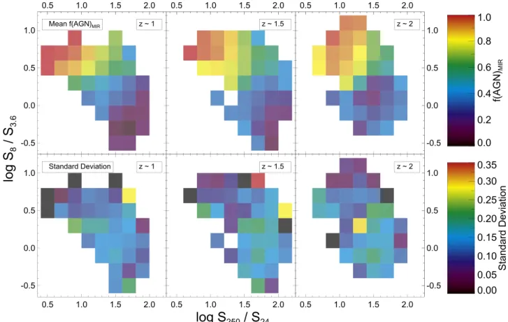
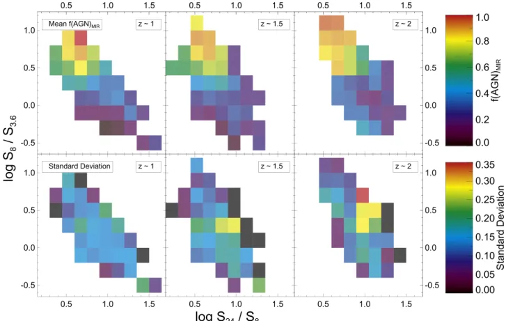
z 0.75 1.25, z=1.25 1.75, and– z=1.75 2.25. Beyond– this redshift, it becomes too difficult to reliably separate Composites from SFGs with these colors. Because only a fraction of CANDELS and COSMOS sources have a SPIRE or PACS detection, we also create a color diagnostic using the colors S24 S8 versus S8 S3.6, although this is slightly less accurate. In each redshift bin, we divide the color space into regions of0.2´0.2 dex and calculate the average f AGN( )MIR and standard deviation, sAGN, of all the synthetic galaxies that lie in that region. In the Appendix, we show our three diagnostics: S250 S24versusS S8 3.6 (used when a galaxy has the appropriate photometry, as it is the most complete at selecting Composite galaxies), S100 S24 versusS S8 3.6 (used when a galaxy does not have a 250μm detection), and S24 S8 versusS S8 3.6 (used for all galaxies without a longer-wavelength detection).

Our color diagnostics assign sources an f AGN( )MIRin bins of Df AGN( )MIR=0.1, but the sAGN of each region is often larger than this(see theAppendixfor a visual representation). Therefore, it is more accurate to broadly group sources as SFGs, Composites, and AGNs. We determine how to group sources by comparing the f AGN( )MIR assigned to each synthetic galaxy by the three different color diagnostics. There is a one-to-one correlation between f AGN( )MIR (250 μm), f AGN( )MIR(100 μm), and f AGN( )MIR(24 μm), with a scatter of s = 0.15. Accordingly, we classify as SFGs sources with f AGN( )MIR <0.30, while the AGNs have

>

( )

f AGNMIR 0.70 and Composites are everything in between.

We assess the completeness and reliability of our color technique by determining how many of our synthetic galaxies are correctly identified as SFGs, Composites, and AGNs in each diagnostic, and we list the completeness and reliability in Table1. In the following definitions, we use Ninputto represent the total number of intrinsic objects(so NAGN,inputis the number of synthetic galaxies that are intrinsically AGNs) and nsel to represent the number of objects recovered by our color criteria (so nAGN,sel is the number of intrinsic AGNs that our color selection identifies as AGNs). Completeness is defined as the

fraction of AGNs (for example) selected: nAGN,sel NAGN,input. Reliability is the fraction of all the sources selected by the diagnostic as AGNs (for example) that actually are, intrinsi-cally, AGNs: nAGN,sel nall,sel. The lower completeness and reliability of the Composites and SFGs are due to these sources being more easily confused with each other when relying on the limited SED coverage(particularly of the mid-IR) provided by 8.0, 24, 100, and 250μm. By adding more bands, MIRI will allow for a more nuanced measurement of the strength of the PAH emission compared with continuum and stellar bump emission. It is also important to note that we are missing AGNs with extreme obscuration, whose IR colors could mimic those of SFGs. We discuss this issue more fully in Section4.1.

We assign each CANDELS or COSMOS source with

= –

z 0.75 2.25 an f AGN( )MIR and associated uncertainty (sAGN) and then broadly group sources into SFGs, Composites, and AGNs. Overall, from CANDELS(COSMOS), 534 (6426) sources have been classified with S250 S24versus S8 S3.6, 864 (175) with S100 S24versus S8 S3.6, and 871 (5360) with

S24 S8versus S8 S3.6. From CANDELS, we also fit an additional 111 sources, which lie slightly beyond the regions (within 0.2 dex) in our color classification scheme, with the Kirkpatrick et al. (2015) template library to determine the

classification. We were unable to classify 3% of sources because they lay outside the regions of our color classification scheme and were not well fit with our template library. This small percentage verifies that our template library is a robust choice and captures the intrinsic variation of dusty galaxies at cosmic noon.

3.1. Galaxy and AGN Counts

Now, we determine how traditional 24μm number counts break down into the SFG, Composite, and AGN categories. We only consider sources with S24>80 Jym , which is the 80% completeness limit(Pérez-González et al.2005). We measure

directly the EGS, COSMOS, GOODS-S, and UDSfield sizes covered by our sources. We show the total CANDELS +COSMOS 24 μm number counts as the open gray stars in

Table 1

Completeness(Reliability) of Redshift-dependent Color Selection

Region _{z~1 z~1.5 z~2} S250 S24versus S8 S3.6 AGN 93(85)% 92(89)% 97(86)% Composite 67(67)% 81(63)% 56(66)% SFG 66(77)% 41(75)% 64(64)% S100 S24versus S8 S3.6 AGN 97(89)% 94(89)% 98(81)% Composite 69(71)% 76(64)% 42(59)% SFG 67(75)% 46(69)% 62(57)% S24 S8versus S8 S3.6 AGN 93(85)% 90(88)% 97(83)% Composite 69(65)% 67(66)% 48(82)% SFG 60(77)% 61(65)% 87(68)%

Note.Completeness is defined as the percentage of sources of a given intrinsic classification that are also selected by the color diagnostic. Reliability (shown in parentheses) is the percentage of all sources classified in a given category where the intrinsic classification agrees.

Figure 1, and these counts are in agreement with the counts from Papovich et al.(2004). In the full COSMOS field, we take

care not to double-count sources in both CANDELS and COSMOS. We plot the 24μm counts at cosmic noon ( =z 0.75 2.25) as the filled black stars. There is a disagree-– ment with the full counts that arises from applying the redshift cut, and this chiefly affects the bright end (S24>1 mJy), which is where AGNs will dominate the counts (Kirkpatrick et al.2013). The lack of bright sources is a result of the small

field sizes of CANDELS (0.22 deg2_{) and COSMOS (2 deg}2_). We show how the cosmic noon counts break down into SFGs (blue), Composites (purple), and AGNs (orange). We have calculated uncertainties on the counts using a Monte Carlo technique, where we vary the f AGN( )MIR for each source within its associated uncertainty and recount sources. We follow this procedure 1000 times. The counts in Figure 1

represent the mean from the Monte Carlo simulations, and the error bars are standard deviations from the Monte Carlo trials and the standard Poisson errors, summed in quadrature.

Below 0.8 mJy, SFGs dominate the counts, but AGNs become more prevalent with increasing brightness. In the bottom panel of Figure 1, we show the percentage of sources above a given flux threshold. We find that AGNs contribute ∼10% at 0.3 mJy and increase to ∼80% at 2 mJy, in good agreement with measurements in Brand et al. (2006) in the

Boötesfield. Although AGNs are frequently assumed not to be abundant in fainter IR samples, the presence of AGN hosts at

m

<

S24 100 Jy was also seen in a small Spitzer/IRS

spectroscopic sample of lensed galaxies at z~2, where the authors found that 30% of the sample had IR AGN signatures and 40% had X-ray AGN signatures(Rigby et al.2008). The

Composites >25% of a sample down to the faintest flux threshold at 63% completeness, which we determined by applying the completeness estimates listed in Table 1 to the number of sources classified with each method. Then, at least 25% of a JWST/MIRI sample will be Composite galaxies, providing a rich data set for probing the AGN/star formation connection at cosmic noon.

4.JWST Color Selection

Color selection is a powerful technique for identifying likely AGNs, Composites, and SFGs. We have done an exhaustive search to identify the best MIRI filter combinations for separating galaxies into these three classes at cosmic noon by creating synthetic photometry in the JWST/MIRI filters from the Kirkpatrick et al.(2015) MIR-based library following the

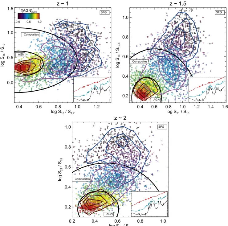
Monte Carlo technique outlined in Section3. As many JWST/ MIRI observations will be carried out infields with available photometric redshifts, or in parallel with NIRcam and NIRspec observations, we include redshift information in our color diagnostics to improve reliability and completeness. We identify three diagnostics covering the ranges z~1 ( =z 0.75 1.25),– z~1.5 ( =z 1.25 1.75), and– z~2 ( =z 1.75 2.25). These three diagnostics, shown in Figure– 2, are different combinations of the S21,S18,S15,S12.8,S10,and S7.7 filters, which cover the 6.2 and 7.7 μm PAH complexes and the 3–5 μm stellar minimum at these redshifts.

We present two methods for separating SFGs, Composites, and AGNs. First, we have determined the optimal AGN, Composite, and SFG regions, labeled in Figure 2. The boundaries of each region are circles, with AGNs lying inside the inner circle, SFGs lying outside the outer circle, and Composites lying in between.

Thez~1 boundaries are

- + - = - + - = ⎛ ⎝ ⎜ ⎞_⎠⎟ ⎛_⎝⎜ ⎞_⎠⎟ ⎛ ⎝ ⎜ ⎞_⎠⎟ ⎛_⎝⎜ ⎞_⎠⎟ ( ) S S S S S S S S

inner: log 0.40 log 0.38 0.25

outer: log 0.35 log 0.45 0.65 .

1 15 7.7 2 18 10 2 2 15 7.7 2 18 10 2 2

Thez~1.5 boundaries are

- + - = - + - = ⎛ ⎝ ⎜ ⎞_⎠⎟ ⎛_⎝⎜ ⎞_⎠⎟ ⎛ ⎝ ⎜ ⎞ ⎠ ⎟ ⎛ ⎝ ⎜ ⎞ ⎠ ⎟ ( ) S S S S S S S S

inner: log 0.49 log 0.18 0.21

outer: log 0.60 log 0.03 0.65 .

2 21 10 2 18 12.8 2 2 21 10 2 18 12.8 2 2

Thez~2 boundaries are

- + - = - + - = ⎛ ⎝ ⎜ ⎞_⎠⎟ ⎛_⎝⎜ ⎞_⎠⎟ ⎛ ⎝ ⎜ ⎞ ⎠ ⎟ ⎛ ⎝ ⎜ ⎞ ⎠ ⎟ ( ) S S S S S S S S

inner: log 0.43 log 0.18 0.18

outer: log 0.50 log 0.12 0.52 .

3 18 10 2 21 15 2 2 18 10 2 21 15 2 2 Figure 1.Top panel: cumulative 24μm number counts for the CANDELS and

COSMOSfields. The open gray stars show the number counts of all 24 μm detected sources, and these agree with the published number counts(Papovich et al. 2004; pink solid line). The filled stars show the 24 μm counts from

= –

z 0.75 2.25. At the bright end, the lack of sources is due to the relatively smallfield sizes. We then show the contribution of SFGs (f AGN( )MIR<0.3; blue circles), Composites (0.3f(AGN)MIR<0.7; purple squares), and AGNs(f AGN( )MIR0.7;orange triangles) to the ~ –z 1 2 number counts. Bottom panel: percentage of each subsample above a givenflux threshold. At

>

S24 0.8 mJy, Composites and AGNs dominate samples. Even at fainter fluxes, JWST/MIRI samples will contain >25% Composites.

These regions are useful for broadly classifying large numbers of sources or identifying targets for follow-up observations. We use these regions to assess the reliability

and completeness of our color diagnostic, where again we classify all synthetic sources as SFGs when f AGN( )MIR <0.3, Composites when0.3f(AGN)MIR<0.7, and AGNs when

 (f )

0.7 AGNMIR. Table 2 lists these values for all three redshift regimes. Comparison with Table1shows an improve-ment over what we were able to reliably classify with the Herschel and Spitzer diagnostics, particularly for separating Composites from SFGs. The spacing of the MIRIfilters allows us to sensitively trace the strength of the PAH features relative to the stellar minimum, where the proportionate amount of PAH emission will be lower for Composite galaxies as the Figure 2.Optimal MIRI color combination for separating Composites, AGNs, and SFGs fromz=0.75 1.25– (top left), =z 1.25 1.75– (top right), and =z 1.75 2.25– (bottom). We show the synthetic galaxies (shaded according to (f AGN)MIR) created from the Kirkpatrick et al. (2015) library used to determine the best AGN and

Composite selection regions(black lines), based on completeness and reliability. We also overplot the contours of all the synthetic galaxies classified as SFGs (blue lines), Composites (purple lines), and AGNs (maroon lines) to allow easier viewing of where each category predominantly lies. In the bottom right corner of each diagram, we demonstrate where the photometryfilters fall on an SFG (black), Composite (blue), and AGN (red) template at =z 1, 1.5, 2.

Table 2

Completeness(Reliability) of MIRI Color Selection

Region _{z~1 z~1.5 z~2}

AGN 87(90)% 87(89)% 87(80)%

Composite 77(72)% 79(74)% 71(71)%

power-law emission from the AGN begins to outshine the stellar minimum(see the insets in Figure2for a visual guide). Perhaps, instead of broad classifications, the reader would rather have an estimate of f AGN( )MIR. Without mid-IR spectroscopy, robust decomposition into an AGN and star-forming component still is not feasible, even with six photometry filters. However, we have determined how to linearly combine the colors in each redshift regime in order to estimate f AGN( )MIR, and we also measure the standard deviation(sAGN) of the residuals when each equation is applied to our synthetic sources so that the reader has a measure of the uncertainty. Atz~1, = - ´ -´ + ⎛ ⎝ ⎜ ⎞_⎠⎟ ⎛ ⎝ ⎜ ⎞_⎠⎟ ( ) ( ) f S S S S AGN 0.97 log 0.10 log 1.29 4 MIR 15 7.7 18 10 and sAGN= 0.15. Atz~1.5, = - ´ -´ + ⎛ ⎝ ⎜ ⎞_⎠⎟ ⎛ ⎝ ⎜ ⎞_⎠⎟ ( ) ( ) f S S S S AGN 0.56 log 0.85 log 1.29 5 MIR 21 10 18 12.8 and sAGN= 0.13. Atz~2, = - ´ -´ + ⎛ ⎝ ⎜ ⎞_⎠⎟ ⎛ ⎝ ⎜ ⎞_⎠⎟ ( ) ( ) f S S S S AGN 0.55 log 1.01 log 1.25 6 MIR 18 10 21 15 and sAGN= 0.16.

4.1. AGN Contributions in Individual Bands

If we have a good understanding of the typical full IR SED of high-redshift galaxies, as well as the scatter in the population, then a single photometric point can be used in conjunction with representative templates to estimate LIR and star formation rates (SFRs). Since PAH molecules are illuminated by the UV/optical photons from young stars, they are a natural SFR indicator and have been extensively used in the literature to probe SFR and LIR (Peeters et al.2004; Brandl et al. 2006; Pope et al. 2008; Battisti et al. 2015; Shipley et al.2016).

Given the coverage of the MIRIfilters, we will now examine how an AGN can affect the 7.7μm PAH feature for the Kirkpatrick et al. (2015) templates used in this work, as any

AGN contribution will need to be corrected for before converting a PAH luminosity to an SFR. We remind the reader that for these templates, the AGN component is represented as a power law with a slope of Fnµl1.5. We

measure the intrinsic L7.7 of each template using PAHFIT (Smith et al. 2007). Then, we measure LMIRI, which is the photometry of the template through the following MIRI filters

at the given redshifts:

m m m m m = = = = = ( ) z z z z z 0, 7.7 m 0.95, 15.0 m 1.34, 18.0 m 1.73, 21.0 m 2.31, 25.5 m. 7

The redshifts mark where the rest-frame central wavelength of eachfilter is 7.7 μm.

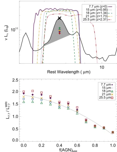
In the top panel of Figure 3, we demonstrate how much of the 7.7μm feature each filter covers at the above listed redshifts. In the bottom panel, we show the relationship

L7.7 LMIRI as a function of f AGN( )MIR for each filter at the listed redshifts. The decreasing fractions with increasing

( )

f AGN MIRare due to the increased contribution of the warm dust continuum to the measured photometry. Wefit a quadratic Figure 3. Top panel: we demonstrate, using the MIR0.0 template from Kirkpatrick et al.(2015), how much of the 7.7 μm feature each MIRI filter

covers at the redshifts where the central wavelength of eachfilter is 7.7 μm (listed in the legend). The gray shaded region indicates which part of the spectrum is integrated to calculate L7.7(black cross), while the filled stars show

the photometry(in units of nLn) measured through each of the MIRI filters. The photometry is lower because it includes more of the spectrum at lower luminosity. Bottom panel: ratio of the MIRI photometry(LMIRI) measured

through different MIRIfilters depending on redshift to the intrinsic L7.7of the

PAH feature. The lower fractions with increasing f AGN( )MIRare due to an

increased warm dust continuum due to heating by an AGN. If L7.7is going to

be used to calculate SFRs, corrections need to be made for an AGN contribution. The black line is the empirical relationship between L7.7 LMIRI

relationship to all the points and measure = -  ´ -  ´ +  ( ) ( ) ( ) ( ) ( ) ( ) L L f f 1.09 0.20 AGN 0.50 0.21 AGN 1.86 0.04 . 8 7.7 MIRI MIR 2 MIR

This equation, in conjunction with estimating f AGN( )MIR from MIRI colors, can be used forfirst-order corrections to L7.7 before converting to an SFR. Similarly, in Kirkpatrick et al. (2015) we demonstrated that there is a quadratic relationship

between f AGN( )MIRand the total contribution of an AGN to

LIR that can be used to correct LIR for AGN emission:

= ´ - ´

( ) ( ) ( )

( )

f AGN 0.66 f AGN 0.035 f AGN ,

9

IR MIR2 MIR

where f AGN( )IR is the fraction of LIR( –8 1000 mm ) due to AGN heating. Then, the portion of LIRdue to star formation is

= ´( - ( ) )

LIRSF LIR 1 f AGN IR . Once the AGN contribution is accounted for, LIR can be converted to an SFR using standard equations (e.g., Murphy et al. 2011). For a strong AGN

(f AGN( )MIR0.9), at least 50% of LIR needs to be removed before converting to an SFR, and the same is true if using

m

7.7 m to calculate SFR. Then, the strongest AGN will have SFRs that are overestimated by at least a factor of 2 if not properly accounted for. Of more concern is Composites, which are routinely misidentified as SFGs. For a Composite with

=

( )

f AGNMIR 0.5, an LIR-based SFR will be overestimated by ∼15%. But, if one uses L7.7, then the resulting SFR will be overestimated by∼35%.

5. Additional Mid-IR Considerations 5.1. Metallicity and Obscuration

At cosmic noon, the bulk of the star formation is occurring in massive, dusty galaxies with M_{* >}1010M (e.g., Murphy et al. 2011; Madau & Dickinson 2014; Pannella et al. 2015),

which is the type of galaxy that our MIRI diagnostics were created from (Kirkpatrick et al. 2012, 2015; Sajina & Yan et al.2012). For studying the AGN–star formation connection,

we expect these types of galaxies to form the most appealing targets. Nevertheless, the sensitivity of JWST/MIRI will enable studies of lower-mass galaxies, which tend to have lower metallicities(Ma et al.2016, and references therein). Decreas-ing gas phase metallicities have been linked with decreasDecreas-ing PAH strengths (e.g., Engelbracht et al. 2008; Sandstrom et al.2012; Shivaei et al.2017), which is a source of concern

since we are effectively detecting AGN hosts based on the strength of PAH features compared with the stellar minimum at 3–5 μm. Shipley et al. (2016) find that below <Z 0.7ZPAH emission no longer scales linearly with LIR, which, based on the mass–metallicity relation, could be a source of concern for contamination of our Composite regions atM_{* <}3´109M, up to z~2.3 (Erb et al. 2006; Zahid et al. 2013; Sanders et al. 2015). Recently, using the MOSDEF optical

spectro-scopic survey, Shivaei et al. (2017) found that at z~2

L7.7 LIR is lower for galaxies with M_{* <}1010M with a behavior similar to that seen for local galaxies (Engelbracht et al.2008; Shipley et al.2016).

Atz~2, a main-sequence galaxy withM_{* =} 1010M will have an SFR of ~45Myr−1(Rosario et al. 2013). At ~z 2, 21μm is tracing the 7.7 μm PAH feature, so applying Equation (11) from Shipley et al. (2016) for this SFR gives

m

»

S21 30 Jy, which is achievable in 7 minutes for a 10σ detection. An hour of integration time at 21μm will produce 10σ detections of galaxies at roughly 8 μJy, corresponding to

* ~ ´ 

M 3 109M _{, which is well below the threshold where}

we expect that low-metallicity galaxies might contaminate the Composite regime. As such, our color diagnostics may require recalibration for low-metallicity galaxies when using observa-tions belowS2130μJy.

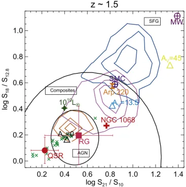
As a visual check, we demonstrate in Figure4where SFGs with different PAH strengths will lie in ourz~1.5 diagnostic. To accomplish this, we use the Small Magellanic Cloud(SMC) dust model (PAH fraction qPAH=0.10%) and a Milky Way dust model with qPAH=0.47% from Draine & Li (2007), which is included to show where a galaxy with a low SFR will Figure 4.We use ourz~1.5 MIRI diagnostic to explore where sources with different luminosities, metallicities, and obscurations from the Kirkpatrick et al. (2015) library will lie in color space; we show the distribution of our synthetic

SFGs(blue), Composites (purple), and AGNs (orange), as well as the black lines marking the AGN, Composite, and SFG regions. We use the Draine & Li (2007) library to calculate where an SMC galaxy (dark purple circle with cross)

and the Milky Way with a lower PAH fraction(purple circle with cross) will lie. The SMC galaxy lies in the Composite region, as well as a galaxy with

= 

LIR 1010L (dark green star) from the Rieke et al. (2009) library. Our diagnostics were calibrated using galaxies with LIR>1011L and

* > 

M 1010M _{, so they should be applied with caution to mass,} lower-luminosity objects. We also look at what effect obscuration may have on our ability to detect AGNs using local obscured ultraluminous infrared galaxy (ULIRG) Arp 220 (orange bowtie) and Compton-thick AGN NGC 1068 (red cross), both of which lie in the Composite region. We use the IRS spectra of optically selected AGNs at z>0.3 (green crosses) from Hernán-Caballero et al.(2015) to show that a range of AGNs lie in our defined region and to the

lower left. Additionally, the empirical quasar template(red circle) and radio galaxy template(pink square) from Leipski et al. (2010) also lie in or below our

AGN region. Finally, we use the AGN template library (triangles) of Siebenmorgen et al.(2015) to show how obscuration in the torus (measured in

AV) combined with a large viewing angle (in this case, 67°) and high cloud filling factor will push AGNs into the Composite and SFG region.

lie. The Draine & Li(2007) models are also parameterized in

terms of the strength of the radiationfield, Umin and Umax. We set these values to Umin=1 andUmax=1 5e , although these parameters have little effect on thefinal colors. Also, we note that we add in a stellar blackbody with T=5000 K to complete the near-IR portion of the spectrum. Even with a low PAH fraction, the Milky Way template still lies in our SFG region, while the SMC template lies directly on the Composite/ SFG border. Haro 11, another well-studied low-metallicity galaxy( =Z 1 3Z; James et al.2013) in the nearby universe, has nearly identical MIRI colors to our plotted SMC data point, further confirming that low-metallicity galaxies will likely lie around the Composite/SFG border. The reason is that even though low-metallicity galaxies have diminished PAH features, they still have a deep and broad stellar minimum at 3 5 m– m (Lyu et al. 2016), unlike Composites, which begin to exhibit

the warmer dust characteristic of the AGN torus. We also plot the template from Rieke et al.(2009), which corresponds to an

=

LIR 1010LIR, as this is an order of magnitude less luminous than the Kirkpatrick et al. (2015) library. A galaxy of this

luminosity also lies in the Composite region, although it is away from the locus of our Composite galaxies (purple distribution).

We caution the reader to be prudent when classifying galaxies as Composites, particularly low-mass sources that lie near the Composite and SFG border. If stellar masses of MIRI samples are known (possibly through NIRcam observations), low-mass galaxies that lie in our Composite regions provide excellent targets for follow-up spectroscopy observations, to distinguish between AGNs and metallicity as the underlying cause of the diminished PAH emission.

The other prominent concern in a mid-IR diagnostic is how obscuration can affect the detection of AGNs. Our template library was built assuming that the AGN can be represented as a power law, and we empirically measure the power-law component to have an average slope ofFn µl1.5, but individual

sources will show a range of slopes and a range of dust obscurations. The AGN templates in the Kirkpatrick et al. (2015) library are derived from AGNs where 75% of the

sample are also detected in the X-ray, implying that they are largely unobscured. Of the Composite sources in Kirkpatrick et al.(2015), only 35% are X-ray detected, indicating that they

contain more heavily obscured AGNs. We now explore the effects of dust obscuration by examining where different galaxies will lie in the z~1.5 color space(Figure4).

Arp 220 (orange bowtie) is a local ULIRG that is heavily dust obscured and may host an AGN (Veilleux et al. 2009; Teng et al.2015). Its position near the SMC and at the edge of

the Composite region indicates another possible ambiguity, that the aromatic bands tend to be suppressed in the most luminous and compact infrared galaxies. How many such objects exist at cosmic noon is not well quantified, as most galaxies of the same luminosity as local ULIRGs (LIR>1012L) have extended ISMs (Papovich et al. 2009; Younger et al. 2009; Finkelstein et al. 2011; Rujopakarn et al. 2011; Ivison et al.2012; Rujopakarn et al.2016). NGC 1068 (red cross) is

an archetypal local Compton-thick Seyfert II AGN. Despite its extreme obscuration, it lies securely in our Composite region, close to the AGN boundary.

The AGNs that our templates were composed of all have remarkable similar mid-IR spectral slopes. To more fully

explore the JWST colors expected of AGNs, we include two literature samples. First, Hernán-Caballero et al.(2015) have

Spitzer/IRS spectra for 189 low-redshift optically selected AGNs. Of these, 24 have z>0.3, so the IRS spectrum covers the appropriate wavelength range for our MIRI diagnostic. These galaxies are shown as the green crosses in Figure 4. They all lie either in our AGN region (with the exception of one galaxy) or to the lower left. Next, we look at the quasar and radio galaxy templates from Leipski et al. (2010). These templates were created from 11 quasars and 9

radio galaxies, respectively, at 1.0< <z 1.4. The radio galaxies are dust obscured with an average t9.7 mm =1.1. In

fact, the radio galaxy template has the same shape as the quasar template viewed through a dust screen with AV=20. The radio galaxy template (pink square) lies in our AGN region, although the s1 dispersion of the sources used to create the template indicates a range of colors that bleeds into our Composite region. The quasar template(red circle) lies to the lower left, and the 1s dispersion is relatively small. Indeed, both the quasar template and some of the IRS AGN spectra lie in a region not occupied by any of our synthetic galaxies(represented by the contours). Sources that lie to the lower left of our AGN regions in any of our diagrams are then most probably bright AGNs.

We also use the AGN library of Siebenmorgen et al.(2015) to

examine what extinction conditions would push an AGN into our SFG region. These AGN templates are calculated assuming that the AGN IR emission arises from a two-phase dust region consisting of a torus and disk, torus radius(R), viewing angle, cloudfilling factor (V_c), optical depth of clouds in the torus (A_V), and optical depth of the disk midplane(A_d). Viewing angle alone can push an AGN into our SFG region, if the angle is greater than 80°. For viewing angles greater than 60°, a high cloud optical depth(AV 13.5) and high filling factor ( >Vc 38%) can also

push pure AGNs into the Composite and SFG regions. We demonstrate how a pure AGN, with no stellar component, can mimic the colors of Composites and SFGs with increasing cloud Figure 5.L2 10 keV– LIRAGNas a function of LIRAGN(all quantities are in erg s−1)

for the four CANDELSfields. We empirically measure the relationship (solid line) using only the GOODS-S data (red circles), since this is the field where the Chandra observations are complete down toL2 10 keV– =1042erg s−1out

to z=2. We show the approximate conversions derived in Mullaney et al. (2011; dotted line), using a local sample of AGNs with L2 10 keV– ~1043

erg s−1, and derived in Elvis et al.(1994; dashed line) from quasars with >

–

optical depth (blue and yellow triangles) for a viewing angle of 67° and Vc=77.7% (we use the model with

= ´ =

R 1545 10 cm15 and Ad 300; changes in these para-meters are not responsible for causing the AGN to lie in the SFG region). Detecting such an obscured AGN at other wavelengths would also be extremely challenging, and identifying complete samples of true Type II obscured AGNs remains an unsolved problem. Del Moro et al. (2016) find that 30% of

mid-IR-luminous quasars at z~ –1 3 in the GOODS-S field are not detected in the Chandra 6 Ms data. Of those that are detected, >65% are Compton thick. Beyond these estimates, it is difficult to say how many heavily obscured AGNs there are that would not be selected as such in the X-ray or the mid-IR. Identifying

these very obscured AGNs will require detailed SED modeling using a full suite of NIRcam+MIRI observations, which is beyond the scope of this paper.

5.2. The 3.3 μm PAH Feature

Atz= –1 2, the PAH 3.3μm feature will fall into the 7.7 and 10μm bandpasses, so it is worth considering whether this feature might also be used as an AGN discriminator. As this is a narrow feature, its effect on a photometric measurement will be much less than the broad 7.7μm complex. For example, Lee et al.(2012) measure the 3.3 μm feature using AKARI near-IR

spectra of local(U)LIRGs, and the largest equivalent width the authors measure is 0.18μm. By comparison, MIRI F770W has

m

D =l 2.2 m. Then, in the most optimistic scenario, the 3.3μm feature will span <10% of the broadband photometry filter. Still, if the PAH emission is particularly strong, it may have a measurable effect on the photometry, and an excess may be observed. However, we note that this PAH feature lies adjacent to water absorption at the 3.1μm, which will also fall in a broadbandfilter and diminish any excess.

Of more concern is the fact that the 3.3μm feature is not uniformly observed, in contrast to the 6.2 and 7.7μm complexes. Sajina et al. (2009) looked for 3.3 μm emission

in 11z~2 galaxies and detect it in only four sources. Lee et al.(2012) do not detect the feature in 11 out of 36 local (U)

LIRGs. Moreover, in both of those samples, the 3.3μm feature fails to exhibit a strong anticorrelation with AGN strength. This is because, at this wavelength range, the emission from the torus is beginning to decrease, but the emission from the accretion disk (which can dominate UV/ optical light) is also weak (e.g., Calistro Rivera et al. 2016, and references therein). Then, any particularly strong dust features from l~0.8 3.5 m are still visible. In fact, in– m Sajina et al.(2009), three of the four spectra that exhibit the

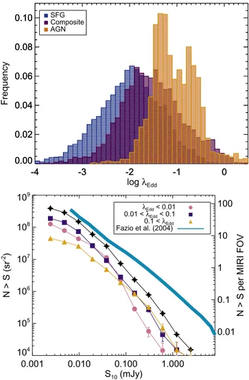
3.3μm emission are all AGNs with f AGN( )MIR >0.7. Of Figure 6.Top panel: we calculate lEddfor CANDELS+COSMOS-identified

SFGs(blue), Composites (purple), and AGNs (orange) by applying standard scaling relations to M*, f AGN( )MIR, and LIR. We have normalized the

distributions to show the relative frequencies in each category. Each category spans an overlapping range, illustrating the current limitations in understanding how observed IR dust emission relates to the accretion on a galaxy’s central black hole. Bottom panel: we predict the MIRI 10μm number counts at

= –

z 0.75 2.25 and then break them into bins of lEdd. We have scaled the

24μm emission of the CANDELS and COSMOS galaxies shown in Figure1

using the appropriate template for SFGs, Composites, and AGNs. Our 10μm counts agree with the measured 8μm counts in Fazio et al. (2004; blue line). The discrepancies between the 10 and 8μm counts can be attributed to the redshift cut. In one MIRI FOV, we will detect nearly 100 galaxies down to 2μJy, and many of these will be AGN hosts.

Figure 7.We show the host galaxy property sSFR=SFR *M of CANDELS galaxies identified as likely AGNs according to a hard X-ray cut (red histogram; L2-10 keV1043 erg s−1) and MIRI color selection (blue histogram). We have normalized each distribution to allow easier comparison, although the MIRI distribution has 20× more sources. The MIRI selection is sensitive to host galaxies with higher sSFRs. We illustrate which of the MIRI-selected AGN hosts would also be MIRI-selected with the Donley et al.(2012) IRAC

selection criteria. Due to the sensitivity and coverage of the MIRIfilters, we will be able to select larger samples of AGN hosts than was possible with IRAC selection.

the 26 sources Lee et al. (2012) detect 3.3 μm emission in,

the authors classify 11 as AGNs based on various near-IR spectral features. Taken together, these points argue against the utility of 3.3μm emission as a color-based discriminator.

6. Discussion: Physical Properties of an MIRI Sample We now return to our CANDELS+COSMOS sample to investigate the physical properties of galaxies that MIRI color selection will identify as being AGN hosts. f AGN( )MIR is strictly a measure of the dust heated by an AGN relative to that heated by star formation, so now we examine a more physically motivated quantity, the Eddington ratio. The Eddington ratio is defined as lEdd= Lbol LEdd, where Lbol is the bolometric luminosity of the AGN and LEdd is the Eddington luminosity. In this way, lEddis a measure of how efficiently a black hole is accreting material. Lbol is commonly estimated from the hard X-ray luminosity, L2 10 keV– . Due to obscuration and varying depths of the Chandra catalogs in the CANDELS fields, we do not have L2 10 keV– for all of our IR identified AGNs and Composites. As afirst step toward calculating Lbol, we estimate

–

L2 10 keVfrom LIR

AGN_{for all sources. We empirically determine} the scaling between these luminosities to be

=  -  ´ -⎛ ⎝ ⎜ ⎞ ⎠ ⎟ ( ) ( ) [ ] ( ) L L L log 31.698 3.535 0.734 0.082 log erg s 10 2 10 keV IR AGN IR AGN 1

measured directly using Chandra observations of the GOODS-S field, which is the only field where the Chandra data are complete down to L2 10 keV– =1042 erg s−1out to z=2 (Xue et al.2011; Hsu et al.2014). Note thatL2 10 keV– is the observed luminosity, as in most cases we do not have high enough counts to make a meaningful obscuration measurement. Figure 5 shows this empirically derived relationship, along with the approximate conversion factors derived in Mullaney et al. (2011), using a local sample of AGNs with

~ –

L2 10 keV 1043 erg s−1, and derived in Elvis et al. (1994) from quasars withL2 10 keV– >1045 erg s−1. Our conversion is in line with the literature results for the brighter AGNs.

We then apply Equation(10) to all sources in the CANDELS

and COSMOS fields. Next, we convert L2 10 keV– to Lbol using Equation (2) in Hopkins et al. (2007). This equation

results in L2 10 keV– Lbol~0.06 0.01– , in agreement with direct measurements in the literature (Vignali et al. 2003; Steffen et al. 2006; Vasudevan & Fabian 2007). Finally,

we calculate LEdd[erg s-1]=1.3´1038´MBH[M], where *

=

MBH 0.002M following the convention in Marconi & Hunt

(2003) and Aird et al. (2012).

With the techniques outlined in Section4, we will be able to calculate lEddfor samples with M*or MBH measurements. The relationship between lEdd and f AGN( )MIR is not linear, since lEdd depends not only on f AGN( )MIR but also on LIR and M_*. Then, each f AGN( )MIR can have a range of lEdd depending on the host galaxy properties. We show in the top panel of Figure 6 the distribution of lEdd for each galaxy category.

In the bottom panel of Figure 6, we illustrate the predicted number counts at cosmic noon with the MIRI 10μm filter,

which is chosen for its sensitivity(~0.6 Jy at 10σ in <3 hr;m Glasse et al. 2015) and because we use it in all three color

diagnostics. We calculate the 10μm flux for all CANDELS +COSMOS galaxies at =z 0.75 2.25 and with– M_{* >}108M by scaling the appropriate Kirkpatrick et al. (2015) template

(based on the source’s (f AGN)MIR determined through color classification) to the available IR photometry and convolving with the 10μm transmission filter. By template fitting, we are also able to calculate LIR and f AGN( )IR. The total 10μm counts are plotted as the black stars in the bottom panel of Figure6. By including lower-mass galaxies, we push below the 80% completeness in Figure 1 and down to the 20% completeness limit(corresponding to~40 Jy at 24 μm). Form reference, the 80% completeness limit (measured at 24 μm) corresponds to S10~10 Jym . Our counts are in good agree-ment at the faint end with the published 8μm galaxy counts in Fazio et al. (2004). At the bright end, we have fewer sources

owing to the redshift cut we imposed and the smallfield sizes, similar to our 24μm number counts in Figure1.

We also break our 10μm number counts into bins of lEdd. Comparison with the top panel demonstrates that the

lEdd< 0.01curve(pink circles) is dominated by SFGs, while the lEdd> 0.1 curve (yellow) has accretion rates typical of sources identified as AGNs at IR and X-ray wavelengths. The majority of the counts are lEdd=0.01 0.1– (purple squares), and these are objects that could be classified as AGNs, SFGs, or Composites.

The MIRI field of view (FOV) is ¢ ´ ¢1. 2 1. 9, so we also illustrate the counts in a MIRI FOV on the right axis of Figure6. We expect nearly 100 objects per MIRI FOV down to 2μJy at 10 μm, achievable at a signal-to-noise ratio of 10(5) in roughly 15 minutes (3.6 minutes). Of these objects, >50% may be AGN hosts where we can detect and measure the black hole accretion. Below S10=10mJy, the counts become dominated by sources with M_{* <}109M. Of the galaxies with lEdd> 0.01, 30% have M_{* <} 109M and compose a prime population for follow-up studies to more concretely pin down the AGN fraction in low-mass galaxies atz~ –1 2.

The above analysis was done assuming spatially unresolved galaxies, but the resolution of MIRI may allow for the detection of AGNs in even lower-lEdd galaxies. For example, at z=1, our color diagnostic requires F1500W, which has a spatial resolution of 0 48. This resolution corresponds to physical scales of 3.8 kpc. Now, at cosmic noon, MBH is more closely tied to M_*rather than bulge mass(e.g., Sun et al.2015), and

very roughly speaking, half of the stellar mass will be contained in the central 3.8 kpc (see size measurements in Rujopakarn et al. 2016). Our color selection can then be

applied to just the central resolution element, which is where all of the AGN emission will emanate from. Then, we will be able to detect galaxies with lEdd that is half of what we have predicted in Figure6.

The use of the lEdd parameter highlights an area where MIRI will enable great strides forward, namely, under-standing how the observable properties of AGN hosts correlate to their physical properties. The broad distributions of lEdd in the top panel of Figure 6 demonstrate the limitations of either broadly grouping sources into AGNs, Composites, and SFGs based on observables or using scaling relations to calculate physical properties, or very likely a combination of the two. But with the high-resolution

spectroscopy on MIRI and the increased number of photo-metric filters, we will be able to classify galaxies on the relative strengths of PAH features, estimate f AGN( )MIR, and combine with M_*(attainable with NIRcam) to measure lEdd, providing clearer insight into the relationship between galaxy dust emission and black hole accretion.

Finally, we demonstrate the host galaxy properties of CANDELS AGNs and Composites selected with different techniques at z~ –1 2 in Figure 7. We calculate SFR for all galaxies byfitting templates from the Kirkpatrick et al. (2015)

library, based on classification as an SFG, Composite, or AGN, and then removing the AGN contribution to LIR before converting to an SFR using Equation(3) in Kennicutt (1998).

We combine SFR with M_* (Santini et al. 2015; Stefanon et al.2017) to measuresSFR=SFR M_*, a common probe of galaxy evolution, as this ratio will be lower in galaxies that are quenching (e.g., Pandya et al. 2017, and references therein). In red, we plot the distribution of specific SFR (sSFR) for those galaxies identified as AGNs in the hard X-ray band (L2 10 kev– 1043 erg s−1). Then, we plot the distribution of sSFR in blue for those galaxies that will be selected as either AGNs or Composites by our MIRI color diagnostics, based on our estimation of their JWST colors through templatefitting. For easier comparison, we normalize both distributions to have a peak at 1, although the MIRI distribution actually has 20×more galaxies than the X-ray distribution. In practice, the relative numbers of X-ray and MIRI AGNs will depend on the depth of the observations and the area covered, but the sensitivity of MIRI and our ability to select Composite sources will enable larger samples than X-ray selection alone. Crucially, our cosmic noon CANDELS AGN hosts have higher sSFR than the X-ray-selected CANDELS galaxies (Azadi et al. 2015; Mullaney et al.

2015). Combining MIRI and X-ray samples will increase our

dynamic range in sSFR, allowing us to explore how black hole accretion varies with star formation and main-sequence location (Mullaney et al. 2012; Rosario et al. 2013; Stanley et al.2015).

Prior to JWST, the most popular way of identifying large samples of IR AGNs is with IRAC color techniques (Lacy et al.2004; Stern et al.2005; Donley et al.2012). The Donley

et al. (2012) IRAC diagnostic is the most reliable, since it

eliminates host galaxy contamination, but it is only sensitive to the most actively accreting AGN as it is based on a power-law selection criterion. Hence, it is likely to be significantly incomplete for Compton-thick and other obscured AGNs. Of the CANDELS sources selected by our MIRI diagnostics, we show in green the sources that are also selected as AGNs by the Donley et al. (2012) criteria.

Clearly, due to the sensitivity and spacing of the MIRIfilters, we will be able to detect >4 times as many AGN hosts as would be identified with IRAC alone. MIRI color selection will enable identification of statistical samples of AGN hosts in their star-forming prime(as measured by sSFR), allowing astronomers to trace the star formation–AGN connection at the peak period of stellar and black hole growth in the universe.

7. Conclusions

We identify SFGs, AGN, and Composites in four CAN-DELSfields and in the full COSMOS field using three different

redshift-dependent color identification techniques. We present the first 24 μm counts of star-forming+AGN Composite galaxies at z~ –1 2. We find that IR AGNs and Composites dominate 24μm samples atS24>0.8mJy. Any 24μm selected sample contains >25% of Composites.

We use a library of SFG, AGN, and Composite templates to create synthetic galaxies, and we use these synthetic galaxies to create JWST/MIRI color selection techniques for three redshift bins,z~1,z~1.5, andz~2. Our techniques can safely be applied to galaxies with M_{* >} 1010M. However, below this regime, metallicity may effect the strength of the PAH features, causing contamination of our Composite regime. MIRI can achieve 10σ detections of * <M 1010Mgalaxies out toz~2 in a matter of minutes, so future JWST observations will prove crucial in separating differences in mid-IR emission due to metallicity rather than AGNs in low-mass galaxies.

At these redshifts, our color selection techniques cover the 6.2 and 7.7μm PAH features and the 3–5 μm stellar minimum, which are robust tracers of star formation. We demonstrate how to correct L7.7for AGN contamination before converting to an SFR, a crucial step or SFRs based on 7.7μm PAH emission will be overestimated by >50% for AGNs and 35% for Composites.

Finally, we predict the Eddington ratios(lEdd), a measure of black hole accretion efficiencies, that we will observe with MIRI imaging. Our MIRI color selection diagnostic can identify samples of AGNs and Composite galaxies with

lEdd> 0.01that are four times larger than samples of AGNs selected by Spitzer/IRAC techniques. We also use our new 24μm number counts to predict the number counts at 10 μm in different bins of lEdd. With MIRI color identification, we will be able to probe the star formation–AGN connection in dusty galaxies at cosmic noon.

A.K. thanks Sandy Faber and Belinda Wilkes for helpful conversations. A.K. gratefully acknowledges support from the YCAA Prize Postdoctoral Fellowship. A.P. and A.S. acknowl-edge NASA ADAP13-0054 and NSF AAG grants AST-1312418 and AST-1313206.

Appendix

In this appendix we show our redshift-dependent color diagnostic tofind SFGs, Composites, and AGNs using Spitzer and Herschel photometry. We create a catalog of 5500 synthetic galaxies from 11 templates where we know the intrinsic AGN contribution. We resample each photometric point within the uncertainties of the template from which it was created, so that we can represent the scatter in color space of real galaxies, which is an improvement on using so-called redshift tracks alone to explore where SFGs, Composites, and AGNs lie in color space.

We create color diagrams in redshift bins ofz=0.75 1.25,–

= –

z 1.25 1.75, and z=1.75 2.25. In each redshift bin, we– divide the color space into regions of 0.2´0.2 dex and calculate the average f AGN( )MIR and standard deviation

sAGN of all the synthetic galaxies that lie in that region. In Figures 8–10 below, we show our three diagnostics:

S250 S24 versusS S8 3.6, S100 S24 versusS S8 3.6, and S24 S8 versusS S8 3.6.

Figure 8. S250 S24 vs. S8 S3.6in three redshift bins. The top panels are shaded according to the averagef AGN( )MIRmeasured in each bin, and the bottom panels

show the standard deviation of f AGN( )MIRfor the sources in each bin.

Figure 9. S100 S24 vs.S8 S3.6in three redshift bins. The top panels are shaded according to the averagef AGN( )MIRmeasured in each bin, and the bottom panels