Studio della fascia costiera e dei mari italiani mediante l'analisi integrata di dati da satellite e in situ

(1)

U

n

i

v

e

r

s

i

t

à

d

i

B

o

l

o

g

n

a

DOTTORATO DI RICERCA IN

Scienze Ambientali:

Tutela E Gestione Delle Risorse Naturali

Ciclo XXIII

Settore Concorsuale 04/A4 - GEOFISICA

Settore scientifico-disciplinare di afferenza: GEO/12

“Studio della fascia costiera e dei mari italiani

mediante l'analisi integrata di dati da satellite e

in situ”

"Satellite and in situ data integrated analysis to

study the upper ocean an coastal environment

of the Italian seas "

Presentata da:

Eleonora Rinaldi

Coordinatore Dottorato

Relatore

Enrico Dinelli

Nadia Pinardi

Co-relatore

Rosalia Santoleri

(2)

2

Acknowledgment

I am very thankful to Dr. Bruno Buongiorno Nardelli, Dr. Simone Colella and Dr. Gianluca Volpe for their patience and scientific guidance in these years.

A special thank you goes to Dr. Rosalia Santoleri for her help, assistance and scientific support.

I thank all the Group for Satellite Oceanography at CNR for making the workplace a friendly place, as well as for their willingness to share experiences and knowledge.

I thank Dr Nadia Pinardi for her insightful scientific discussions. Thank you to my family for having always believed in me.

This thesis is dedicated to Andrea, Fabrizio and Lucrezia who will be born soon. They make my life happy.

(3)

3

Index

Introduction ... 6

Chapter 1 ... 10

Italian seas and coasts ... 10

1.1 The Mediterranean Sea ... 10

1.2 The Tyrrhenian Sea ... 12

1.3 The Sicily Channel... 15

1.4 Ocean Colour Chlorophyll trends along the Italian coasts... 18

Chapter 2 ... 20

Satellite Oceanography ... 20

2.1 Principles of oceanography satellite ... 20

2.1.1 Ocean Colour ... 21

2.1.2 Sea Surface Temperature ... 23

2.1.3 Sea Surface Height... 25

2.2 Use of satellite data to infer information on the upper ocean circulation and dynamics ... 27

Chapter 3 ... 30

Lagrangian and Eulerian observations of the surface circulation in the Tyrrhenian Sea ... 30

3.1 Data ... 31

3.1.1 Drifting buoy data-set ... 31

3.1.2 Wind data ... 34

3.1.3 Altimeter data-set... 35

3.2 Analysis of the surface circulation ... 36

3.2.1 Surface circulation revealed by drifters trajectories ... 36

3.2.2 Pseudo-Eulerian analysis of drifter data ... 39

3.2.3 Overview of the surface circulation as described by the altimeter data ... 41

3.3 Joint pseudo-Eulerian analysis of altimeter and drifter data ... 43

3.4 Seasonal variability ... 46

3.5 Conclusions ... 49

Chapter 4 ... 51

Phytoplankton distribution and variability in the Sicily Channel as seen by remote sensing data ... 51

4.1 The Data ... 52

4.1.1 Chlorophyll data ... 52

4.1.2 SST ... 52

(4)

4

4.2 Methods ... 53

4.3 Results ... 56

4.3.1 Climatological coupling between Chl, and SST and KE ... 56

4.3.2 EOF analysis ... 58

4.3.2.1 The role of Modified Atlantic water over the CHL seasonal variability (1st CHL mode) ... 58

4.3.2.2 Role of the stratification process on the CHL variability at annual scale (2nd CHL mode) ... 61

4.3.2.3 Response to high frequency atmospheric events (3rd CHL mode) ... 63

4.3.2.4 Response to Coastal upwelling (4th CHL mode) ... 64

Chapter 5 ... 68

Ocean Colour Chlorophyll trends along the Italian coasts ... 68

5.1 Data ... 68

5.1.1 In situ dataset ... 68

5.1.2 Ocean Colour dataset ... 69

5.1.2.1 OC Mediterranean re-analysis product ... 70

5.1.2.2 Merged Case 1- Case 2 chlorophyll product ... 70

5.2 Methods ... 71

5.2.1 Ordinary Least Square regression ... 71

5.2.2 Mann-Kendall test... 72

5.2.3 Seasonal Kendall test ... 73

5.2.4 Sen’s Method ... 73

5.2.5 Spearman partial rank correlation test ... 73

5.3 Results ... 74

5.3.1 Comparison between in situ and OC data ... 74

5.3.1.1 Results in the test area ... 74

5.3.1.2 Results along the Italian coasts ... 81

5.3.2 Chlorophyll trend along the Italian coastal and shelf region ... 84

Chapter 6 ... 89

Conclusion ... 89

Appendix A ... 93

(5)

5

Abstract

The thesis objectives are to develop new methodologies for study of the space and time variability of Italian upper ocean ecosystem through the combined use of multi-sensors satellite data and in situ observations and to identify the capability and limits of remote sensing observations to monitor the marine state at short and long time scales. Three oceanographic basins have been selected and subjected to different types of analyses.

The first region is the Tyrrhenian Sea where a comparative analysis of altimetry and lagrangian measurements was carried out to study the surface circulation. The results allowed to deepen the knowledge of the Tyrrhenian Sea surface dynamics and its variability and to defined the limitations of satellite altimetry measurements to detect small scale marine circulation features. Channel of Sicily study aimed to identify the spatial-temporal variability of phytoplankton biomass and to understand the impact of the upper ocean circulation on the marine ecosystem. An combined analysis of the satellite of long term time series of chlorophyll, Sea Surface Temperature and Sea Level field data was applied. The results allowed to identify the key role of the Atlantic water inflow in modulating the seasonal variability of the phytoplankton biomass in the region. Finally, Italian coastal marine system was studied with the objective to explore the potential capability of Ocean Color data in detecting chlorophyll trend in coastal areas. The most appropriated methodology to detect long term environmental changes was defined through intercomparison of chlorophyll trends detected by in situ and satellite. Then, Italian coastal areas subject to eutrophication problems were identified. This work has demonstrated that satellites data constitute an unique opportunity to define the features and forcing influencing the upper ocean ecosystems dynamics and can be used also to monitor environmental variables capable of influencing phytoplankton productivity.

(6)

Introduction

6

Introduction

The oceans cover over 70% of Earth's surface and representing over 95% of the biosphere they contribute to the mitigation of climate change. The oceans are the main reserve and distributor of heat and salts, they affect the weather, modulate evaporation, precipitation and vapour in the atmosphere. The intensification of human activities in coastal areas, in combination with climate changes that are occurring on a global scale, is dramatically altering the biodiversity of marine environments. The forecast of global change include both direct and indirect effects on the structure and functioning of the oceans, including the alteration of the circulation of water masses (Shaffer et al.,2000) and changes in the composition of living communities.

In recent decades the planet’s temperature is increasing (IPCC, 2007), this increment of the temperature is caused by the progressive increase of anthropogenic CO2 (a greenhouse gas)

concentration in the atmosphere (Cox et al., 2000; IPCC, 2001; Sarmiento et al., 2004). The oceans play a fundamental role in the carbon cycle as the concentration of CO2 is in dynamic

equilibrium with that in the atmosphere: an increase in the atmospheric concentration of CO2

enhances the ocean absorbing capacity. The exchange of CO2 between atmosphere-ocean

occurs through the so-called biological pump. Its refers to the sinking of organic matter from the surface productive layers to deep waters in the oceans.

The efficiency of the biological pump is linked to the photosynthesis process that in the marine environment is performed by phytoplankton (i.e., the unicellular microscopic algae living in the upper layer of all water bodies across the world). The phytoplankton through photosynthesis, allows the transformation of inorganic carbon into organic carbon and its storage in biomass. The speed with which this biomass is created and made available to the successive trophic levels is called primary production. Quantifying the carbon flux into the ocean through the marine primary productivity, and understanding the mechanisms that might control it, are of crucial importance for defining the planet’s carbon budget and its link to climate change.

In recent years the science has intensively concerned to understand what are the processes that regulate the global carbon cycle and how the CO2 fluxes between the atmosphere and other

compartments of the planet vary over time. Moreover a lot of effort has been made to understand the physical processes affecting the spatial distribution and temporal development

(7)

7

of phytoplankton biomass. The growth-limiting factor of phytoplankton is the availability of light and nutrients (Parsons et al., 1983). Those depend in turn on physical processes such as general ocean circulation, deep water formation, mixed-layer dynamics, upwelling and the solar cycle (Behrenfeld et al., 2006). It is so obvious the importance of study and understand the phenomena that determine the nutrient enrichment in the surface layers of water as the Sea Surface Temperature and the marine circulation. This later other than have influence on nutrient budget are able to condition the dynamics of the biomass of some pelagic fish species (Cutitta et al.,2003, Garcia Lafuente et al.,2003). A detailed knowledge of the marine circulation is therefore of crucial importance for the correct management of fisheries activities and more generally for the study of the pollution dispersion and transport.

Satellite data represent an essential observational tool which offers an unique perspective on the natural environment. Thanks to the synoptic view and the high sampling frequency and high spatial resolution, remotely sensed data have been successfully used to provide unique and important information on surface phytoplankton distribution, Sea Surface Temperature and sea surface currents. However, the satellites investigate only the first layer of the sea, furthermore, the presence of clouds over the area of acquisition affects the availability of satellite data in the visible and infrared bands. The integration between in situ measurements and satellite observations permits to overcome the inherent limitations of both methods of data collection. Indeed, the in situ measurements, are able to sample the entire water column and to be operational even when the satellite due to cloud cover, is not able to give information about the sea area investigated. Nevertheless, due to the fact that they are point data, the coverage of a large portion of the sea requires long operation times.

The two main objectives of this work are:

1) to develop new methodologies for studying the space and time variability of Italian upper ocean ecosystem through the combined use of multi-sensors satellite data and in situ observations;

2) to identify the capability and limits of the of remote sensing observations to monitor the marine state at short and long time scales.

Three different oceanographic basins have been selected and subjected to different types of analysis.

The first region examined is the Tyrrhenian Sea. This basin has been chosen because all the previous studies indicate that the Tyrrhenian basin is an extremely active region of the Mediterranean Sea, characterized by a rich mesoscale dynamics. Moreover, even if the Tyrrhenian Sea is a basin of transition for the water masses that through it reach the north

(8)

Introduction

8

western regions of the Mediterranean Sea, all the previous study result do not allow an adequate evaluation on the role of this basin plays in the general Mediterranean Sea circulation. The peculiarity of the study done in this thesis is a comparative analysis of altimetry and lagrangian measurements. This method allows to complement and compare the information provided by two datasets separately and aiming to quantify the impact of the different sampling strategy of the two instruments. The purpose of this analysis was to deepen the knowledge of the Tyrrhenian Sea surface dynamics and its variability.

The channel of Sicily was chosen because it plays a key role for the exchange of water masses and their physical-biochemical properties between the Eastern and the Western Mediterranean. Thus, it represents a crucial area for both understanding the basin scale variability and for the important fishery activities carried out by the countries bordering the Channel. The study on this region aims to identify the spatial-temporal variability of phytoplankton biomass and to understand the impact of the upper ocean circulation on the marine ecosystem. To achieve this objectives an combined analysis of the satellite of long term time series of chlorophyll ( the most widely used proxy for the study of the distribution of phytoplankton biomass), Sea Surface Temperature and Sea Level field data was applied. The last region examined is the Italian coastal marine system. Despite the ecologically and socio-economically importance of this area there is a strong scientific consensus that coastal marine ecosystems, along with the goods and services they provide, are threatened by anthropogenic and global climate change. This thesis explores the potential capability of Ocean Color data in detecting chlorophyll trend in coastal areas, indeed remotely-sensed data provides a method to examine trends in the coastal environment without the necessity of in situ sampling observations. It should be noted that, despite the fact that the Sea-viewing Wide Field-of-view Sensor (SeaWiFS) provides ten years of nearly continuous, consistent and reliably-calibrated record of remotely-sensed chlorophyll, in coastal waters remotely-sensed data are less accurate than in the open ocean due to increased turbidity in coastal waters and possible the bottom reflectance problems. For this reason, before to determine the trend of chlorophyll through the satellite data a comparison between them and in situ data was made. The thesis is organized as follows: chapter 1 presents and overview of the Mediterranean Sea circulation and reviews the present main knowledge physical and biological oceanography of the three study areas. In Chapter 2, the basic physical principles of ocean remote sensing are described. Moreover a short state of the art of satellite oceanography is presented. Chapter 3 presents the comparison between langrangian and altimeter data in the Tyrrhenian Sea and the surface circulation as revealed by both dataset is descripted. Chapter 4 shows the

(9)

9

phytoplankton biomass space-time variability in the Sicily Channel and its dependence from physical forcing as Sea Surface Temperature and surface geostrophic circulation. In Chapter 5 the analyses to detect chlorophyll trends along the Italian coasts from Ocean Colour data is investigated. Moreover the phytoplankton trends along the Italian coast was discussed. Finally, Chapter 6 draws the main conclusions of this thesis.

(10)

Italian seas and coasts

10

Chapter 1

Italian seas and coasts

This chapter overviews the state of the art of the Italian Sea oceanography and of the study regarding the chlorophyll trend along the Italian coasts.

First an overview of the Mediterranean sea oceanography is presented, then the state of the art of each geographic area examined in this thesis is discussed.

1.1 The Mediterranean Sea

The Mediterranean Sea (MED) is a semi-enclosed basin connected to the Atlantic Ocean through the Gibraltar Strait. It is divided into two main sub-basins, the Eastern (EMED) and Western (WMED) Mediterranean by the strait of Sicily. Its circulation is schematically decrypted as a three-layer system: the surface layer, that is 50-200 m thick, the intermediate layer, that occupies a thickness between 200 and 600 m and the deep layer (Lacombe and Tchernia, 1972; Lacombe et al., 1981).

The Atlantic Water (AW) enters through the Strait of Gibraltar at the surface, this “sweet” water east of the Strait due to evaporation and mixing increases its salinity migrating to the Levantine Basin (Fig 1.1 a). The temporal scales of this thermohaline circulation is approximately 100 years (Roether and Schlitzer,1991). During winter, when strong winds intensify evaporation producing a process of vertical convection, in correspondence of the Rhodes cyclonic gyre the MAW sinks give origin to the Levantine Intermediate Water (LIW) ( Malanotte-Rizzoli e Hecht,1988; Lascaratos et al., 1993) (Fig 1.1 b).

Different processes of transformation of surface water in deep water characterize the EMED and WMED, however in both basin these process have a sub basin scale and they are characterized by cyclonic circulation (Fig 1.1 c). (Gascard, 1978; Anati, 1981).

In particular, in the EMED the increase in density, which determines the sinking of surface waters, is due to the increase of salinity resulting from the evaporation. An exception is represented by the Adriatic Sea, in which the deep water is originating by a cooling process due to the Bora, a particularly cold and dry wind that blows with extraordinary intensity. This dense water flows along the Italian coast and it mixes with LIW in the Ionian, giving rise to one of the main sources Mediterranean abyssal water. Another site of formation of

(11)

11

intermediate and deep water in EMED is located in the northern Aegean in correspondence to the vortex in the south of Rhodes, as written previously.

In the WMED the deep water is formed by heat loss and subsequent sinking of the waters due to the presence of cold winds. This phenomenon occurs in the Gulf of Lion due to the Mistral wind (Benzohora e Millot,1995; Millot,1999;Rhein et al.,1999), and in the Thyrrhenian Sea (Hopkins,1985).

Figure.1 Schemes of the Mediterranean Sea surface layer(a), intermediate layer (b) and deep layer (c) (from Millot, Taupier, 2004).

(12)

12

1.2 The Tyrrhenian Sea

Although the main characteristics of the Mediterranean Sea are well known, our knowledge of the processes taking place in one of its sub-basins, the Tyrrhenian Sea, is not yet fully exhaustive.

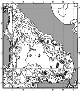
The Tyrrhenian Sea is one of the major sub-basins of the Mediterranean. It has a triangular shape and a very complex bathymetry and is connected to the outer Mediterranean Sea with the Corsica Channel (north) and a broad opening to the south-west, between Sardinia and Sicily (Fig 1.2). This basin plays an important role in the transformation of the main Mediterranean intermediate and deep waters (Astraldi and Gasparini, 1994, Gasparini et al., 1999, Sparnocchia et al., 1999) occasionally resulting in the formation of Tyrrhenian dense water (Astraldi and Gasparini, 1994).

Figure 1.2 Bottom topography of Tyrrhenian Sea.

Even though the first investigations on the Tyrrhenian date from hundred years ago (Nielsen, 1912) and the basin was the object of a thorough investigation carried out in the framework of the International Geophysical Year (Aliverti et al.,1968), direct measurements of velocities and transports in the Tyrrhenian Sea are still very sparse. Available information are mainly based, on one hand, on the in-situ measurements collected in the north part of the basin during “TEMPO” surveys in the late ‘80s/early ‘90s (Astraldi and Gasparini, 1994, and Marullo et al., 1994) and by the limited data collected at its southern entrance by Sparnocchia et al.(1999).

(13)

13

These data allowed a satisfactory hydrological characterization of the Tyrrhenian Sea, even though the mechanisms of observed long term changes still have to be fully understood. On the other hand, the informations on the circulation in the basin, especially at the surface, are much less accurate. The traditional concept (Millot, 1987 and 1999) of a cyclonic circulation at all levels appears to be far too schematic: recent Eulerian (for the deep layer, P. Falco, personal communication on unpublished data) and Lagrangian studies (we refer in particular to the MedArgo data regarding the intermediate water circulation, Poulain et al., 2007) show a remarkable and unexpected complexity. northern portion of the basin where TEMPO data were available, whereas the southern part has not been practically explored.

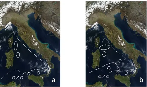
In the past, efforts have been concentrated on some elements of the surface dynamics of the the northwest Tyrrhenian is dominated by the presence of an important feature, the North Tyrrhenian Cyclone (NTC, see Marullo et al., 1994), induced by strong north-westerly winds channelled by the Strait of Bonifacio, presenting a strong seasonal variability and affecting the coastal currents flowing along the north-eastern flank of the basin. Past observations show that this northern gyre, whose dimensions are of the order of 100 km, displays a strong seasonal dependence in size and position. During winter it is stretched along the meridional direction in the western part of the basin, while in summer it is zonally oriented (Artale et al.,1994, Astraldi e Gasparini, 1994) capturing a weak flow along the Italian Peninsula (Fig 1.3 a,b)

Figure 1.3 Reconstruction of the surface circulation of Tyrrhenian Sea during winter-spring (a) and in summer-autumn (b)

(14)

14

n summer, both cyclonic and anticyclonic eddies with characteristic length scales of 30-40 km are nested within the larger gyre (Artale et al.,1994). Marullo et al (1994), on the basis of AVHRR thermal images analysis, suggested that the NTC in summer consists of a cold water filament originating from the Strait of Bonifacio and extending eastward, rather than being a well organized cyclonic structure. Despite this different interpretation of the NTC structure past studies agree that the change of NTC orientation (zonal/meridional in summer/winter) is due to the strengthening of the current that drives the circulation through the Corsica Channel. South of the NTC, an anticyclonic gyre (NTA, North Tyrrhenian Anticyclone) is present. The generation and evolution of these gyres is also controlled by the strong wind events affecting the Strait of Bonifacio, and specifically by the wind stress curl associated with the easterly winds, and its associated Ekman pumping (Crepon et al., 1989; Artale et al. 1994).

The seasonal variability of the northern Tyrrhenian is also mirrored in the water exchange between the Tyrrhenian and the Ligurian Sea, mainly driven by steric effects, which dominate in the winter season (Astraldi and Gasparini, 1994; Marullo et al., 1994; Vignudelli et al., 1999; 2000), with an interannual variability possibly linked with regional teleconnection phenomena, namely the North Atlantic Oscillation (Vignudelli et al., 1999).

In the southern part of the basin, the dynamics are conditioned by the exchanges through the straits of Sicily and Sardinia. Surface water of Atlantic origin (AW) enters the Tyrrhenian Sea off the northern Sicilian coast. (see, e.g., Krivosheya and Ovchinnikov, 1973). It is believed to flow eastwards along the northern coast of Sicily, following an overall cyclonic pattern, proceeding along the western coast of Italy and then entering the Ligurian Sea through the Corsica Channel (Aliverti et al. 1968; Elliot et al., 1978; Tait, 1984). Using Lagrangian data collected in the Straits of Sicily in the 1990s, Poulain and Zambianchi (2007) recently showed that waters coming from the Algerian Current indeed flow north-eastwards into the Tyrrhenian, along the Sicilian coast. Their analyses clearly indicated that this flow returns southbound on the western side of the Sardinian Channel and forms a rather stable cyclonic gyre.

(15)

15

1.3 The Sicily Channel

The Sicily Channel divides the Mediterranean Sea into two sub-basins, the eastern and the western, thus representing a crucial area for both understanding the basin scale variability (Astraldi et al., 1999), and for the important fishery activities carried out by the countries bordering the Channel. The main characteristics of the Channel of Sicily circulation are well known, while the biological processes taking place in the channel and the spatial and temporal distribution and variability of the chlorophyll field still need investigations.

The average depth of the Sicily Channel is less than 300 m, with maximum values not exceeding 1500 m (Figure 4).

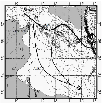
Figure 1.4 Reconstruction of the Sicily Channel surface circulation

From a dynamical point of view, the Sicily Channel can be schematically considered as a two-layer system: a surface (up to ~200 m depth) and fresher water mass (relative to the Mediterranean resident water masse) of Atlantic origin (Modified Atlantic Water, MAW) flowing eastwards, and the saltier Levantine Intermediate Water (LIW) flowing westwards. Once the MAW enters the Channel, near Cap Bon (Figure 4), it splits into two veins, the Atlantic Tunisian Current (ATC) that circulates close to the Tunisian coasts (Beranger et al., 2004, Pierini and Rubino, 2001) and the Atlantic Ionian Stream (AIS, Robinson et al., 1999), that flows into the central and northern region of the Channel (Poulain and Zambianchi, 2007) describing a cyclonic gyre around the Adventure Bank named ABV (Robinson et al., 1999).

(16)

16

South of Pantelleria Island, the AIS often bifurcates: a principal vein flows north-north-eastward, while a weaker stream directly flows along the Tunisian shelf (Lermusiaux et al., 2001). In summer the first veins of the AIS above descript is constrained in the centre of the channel by the up-welling front originating in the southern coasts of Sicily due to with local wind (Buongiorno Nardelli et al., 1999, Marullo et al., 1999a,b Le Vourch et al., 1992; Kostianoy, 1996; Piccioni et al., 1988, Sorgente et al , 00 ranger et al., 2004). On the contrary down welling processes are founded along the eastern coast of Tunisia on the opposite side of the Strait (Agostini and Bakun, 2002). The up-welling front is characterized by jets and filaments that are usually observed off-shore of Mazzara del Vallo and Capo Passero, see Figure 1.5 (Buongiorno Nardelli et al., 1999). During winter, the AIS extends in a wider region because in this season the up-welling is restricted both spatially and temporally.

Figure 1.5 AVHRR images on 9 September 1995 in which are visible the coastal upwelling in the northern part of the channel and two filaments near Mazara del Vallo at 37.3°N, 13.5°E. ( From Buongiorno Nardelli et al., 1999)

Off shore Cape Passero the AIS follows a cyclonic vortex called Ionian Shelf Break Vortex (IBV), (Lermusiaux,1999; Robinson et al., 1999; Lermusiaux and Robinson, 2001). Another cyclonic vortex called Messina Rise Vortex, MRV, is found south of Messina. At the eastern boundary of these latter two vortices the Ionian slope fronts, ISFs, are present and active at different locations and depths (Lermusiaux, 1999 and Lermusiaux and Robinson (2001).

(17)

17

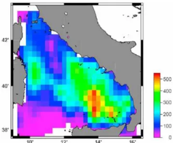
From the biogeochemical point of view the eastern and the western regions of the Mediterranean Sea have already been shown to have an order of magnitude difference in the surface chlorophyll concentration (Santoleri et al., 2008,Volpe et al., 2011) along with different seasonal cycles: the eastern basin presents a seasonal cycle similar to that of the sub-tropical gyres, whereas the western basin phytoplankton dynamics can be associated with that of the north Atlantic with a pronounced spring bloom (D'Ortenzio and Ribera d'Alcalà, 2009). Based on SeaWiFS data, the entire Sicily Channel is characterized by phytoplankton biomass values ranging between 0.04 and 0.5 mg CHL m-3 at sub-basin scale (the entire sub-basin can be considered as a mesotrophic area), with a spatial variability on a daily basis encompassing 3 orders of magnitude (roughly between 0.01 and 10 mg CHL m-3) on a daily basis. In general, maximum (minimum) values recur during winter-spring (summer) in correspondence of periods of low (high) water column stratification. From the visualization of daily SeaWiFS data, higher and nearly invariant values throughout the year are found in coastal areas, whereas off-shore region exhibit a more pronounced variability. Moreover, specific oceanographic features, such as wind-induced coastal upwelling, frontal meanders and instabilities significantly modulate the local distribution of phytoplankton biomass. In fact, the most productive area of the Channel has been generally associated with the up-welling that occurs along the south-eastern coasts of Sicily, at Cape Passero as demostrated by the value of fluorescence found in this area by Lafuente et al (2002) see fig 1.6.

Figure 1.6 Depth of the maximum of fuorescence (meters, labelled contours) and numerical value of this maximum during the period 24 June-14 July 1998 ( from Lafuente et al 2002)

(18)

18

1.4 Ocean Colour Chlorophyll trends along the Italian

coasts

The achievement of a good ecological status in European waters by 2015 is the intent of the Water Framework Directive (WFD) 2000/60. Since the publication of the WFD the European States need an effective monitoring system of the coastal waters. The problem of protection and of a compatible development of coasts necessarily requires a physical and bio-ecological definition of this term, indeed, the coastal areas can be placed in a wide range of definitions so a definition universally valid is difficult to found. The different definitions of coastal take into account separately geomorphological criteria, hydrographic criteria, the economic dynamics or criteria for the distribution of vegetation. For example, the simplest definition refers to the area between the high and low tide, while biologically the bound of the coastal areas is made to coincide approximately with the depth range of 50 m (euphotic zone), in other words how far the Posidonia can survive.

From the Ocean Colour (OC) point of view the waters are usually divided into two categories: case 1 waters, that are those waters in which the optical properties are dependent on the phytoplankton and on the degradation products their associated and case 2 waters in which other substances, such as resuspended sediments, terrigenous particles, yellow substance or anthropogenic materials, range independently from the concentration of phytoplankton and they determine the optical properties of the body of water. Case 1 waters are associated with the open sea waters while case 2 waters are associated with shelf and coastal waters.

The coastal waters represent only a small fraction of natural waters on the planet. However they play a role of great importance from the ecological, social and economic point of view. Indeed about 60% of the world population lives in coastal areas and about 90% of the catch comes from coastal areas. The strong anthropization, the irrational exploitation of resources and the changes in climate, are causing a strong modification of the coastal areas and they represent a continuo threat to the biodiversity of these areas. The eutrophization is the principal risk for the coastal water, it was defined by Nixon (1995) as an increase in the rate of supply of organic matter to an ecosystem’ The degenerative process is caused by the enrichment of water by salts, primarily nitrogen and phosphorus, leading to increased algal productivity and the production of a quantity of biomass greater than that can be used by

(19)

19

herbivorous organisms, this can lead to a reduction of dissolved oxygen when the organic matter decomposes.

For these reasons monitoring of coastal chlorophyll-a (Chl-a) concentration, considered as a proxy of phytoplankton biomass, can be an efficient tool to evaluate the Italian environmental policy taken to reduce the release of nitrogen and phosphate on the coastal water.

The Mediterranean Sea is characterized by a general decreasing trend in Chl concentration (Behrenfeld and al, 2006 Doney 2006and Greget et al., 2003). Behrenfeld et al. (2006) have linked the decreasing trend in ocean primary production to the climatic changes that determine a surface warming, resulting in an increase in the density contrast between the surface layer and underlying nutrient-rich waters. This in turn leads to enhanced stratification, which suppresses nutrient exchange through vertical mixing. Barale et al., (2008) have attributed the negative trend to the increased nutrient-limitation, resulting from reduced vertical mixing due to a more stable stratification of the basin, in line with the general warming trend of the Mediterranean Sea. However they found positive trend of Chl in some coastal area, they have associated this hotspots continental runoff and to a growing “biological dynamism” at these sites

Actually the studies regarding the Chl-a trend along the Italian coast are principally concentrated in the north of the Adriatic Sea. Obviously this is due to the presence of the outflows of Po, which affects the amount of nutrients in this region. A recent study based on satellite data demonstrate that in the last decade there is a decrement of the Chl-a surface concentrations specially in the western area of the basin that is generally more eutrophic respect to the centre and the eastern coast in which the negative trend is less marked (Mozetič et al., 2010). This negative trend is justified by the reductions observed in the outflows of the Po (Zanchettin et al. 2008) and Isonzo (Comici and Bussani 2007) rivers and by the fact that phosphorus being banned by Italian law in the mid-1980s and this , could have had a strong influence on nutrient concentrations in the coastal area (de Wit and Bendoricchio 2001). On the contrary increasing trend of productivity were found in the Middle and Southern Adriatic (Marasoviæ, et al., 1995). More recently, Matarrese et al (2009) analyzing Chl-a Modis data in the Soutern Adriatic Sea found a positive trend in Taranto Gulf and along the Margherita di Savoia coasts. These trend are mostly due to the meteorological forcing, which influenced oceanographic phenomena like water stratification, upwelling, stronger inflows of Mediterranean water into the Adriatic (Morovic et al., 2004).

(20)

Satellite Oceanography

20

Chapter 2

Satellite Oceanography

This thesis analyzes chlorophyll, sea surface temperature and sea level height products derived by satelllite data acquired by both passive and active sensors. These satellite data are produced by specialized processing chains which use specific algorithm for the parameter retrievals. Even if the retrieval of the parameters is out the scope of the thesis, this chapter introduces the basic physical principles of ocean remote sensing. This preliminary step is particularly useful and important to recognize the complexity of the measurement techniques and data processing used to retrieve the geophysical products used in this thesis and to understand some problems encountered in the analysis of the satellite data products. Then potential use of satellite data to infer the upper ocean dynamics and to study the seasonal and interannual variability of the ocean field is review in order to show state of the art of satellite oceanography.

2.1 Principles of oceanography satellite

The first artificial satellite was launched in 1957 by the Soviet Union, and in 1964 there was a first conference in which the possibility of conducting oceanographic observations from space is discussed. To observe the oceans from space allows the synoptic view in two dimensions with high spatial resolution and it makes possible to measure large areas also isolated of ocean for long periods.

The remote sensing sensors measure the electromagnetic radiation emitted or reflected by the area observed at frequencies established (Fig 2.1). The satellite sensors can be of two types: active and passive. The active sensors produce the radiation that are reflected from the surface and then analyzed by the same sensor. Differently, the passive sensors measure the reflection (or emission) of natural radiation on the Earth surface to certain wavelengths.

(21)

21

Figure 2.1 Spectrum bands used for remote sensing (Robinson 2004)

2.1.1 Ocean Colour

The relevant parameters for the OC are the Irradiance, the Radiance, the Reflectance and the Transmittance.

The Irradiance, E, is defined as the amount of radiant energy intercepted by a surface area element. It denotes the light arriving on a surface area and has units of W m-2.

The Radiance, L, is the measure of the light leaving a surface per unit solid angle in a given direction. The radiance has units of W sr-1 m-2.

The Remote Sensing Reflectance of a water body, Rrs, is defined as the Radiance to Irradiance ratio, that is the amount of light leaving the surface vertically upwards weighted by the amount of light entering the surface from all directions. The spectral shape of Rrs defines the so-called ocean colour.

The Transmittance ,T, is the fraction of radiation that passes through a medium which absorbs uniformly.

Only a small percentage of the signal received from the sensor comes from the ocean. Indeed the 80-90% of the signal is due to the interaction of the electromagnetic waves with the constituents of the atmosphere as molecules (Rayleigh) and particles (Austin, 1974 ; Hooker et al., 1992).

Figure 2.2 shows the radiance that reaches the sensor at the top of the atmosphere and it is made of various contributions as proposed by Gordon (1978, 1981) T’LW is the

(22)

water-Satellite Oceanography

22

leaving radiance inside the Instantaneous Field Of View (IFOV) plus the radiance that arise the sensors from the external water of the IFOV but that is captured as a result of scattering of the atmosphere. LR and LA are the radiances due to the molecular scattering (Rayleigh) and

aerosol scattering respectively.

Figure 2.2 Optical pathways to an ocean colour sensor

Defining LS as the total radiance received to the sensor, we can write:

LS = LA+ LR+ T LW 1.1

LR can be estimated with sufficient accuracy for remote sensing applications using the theory

of Rayleigh (Gordon et al., 1988a) while the estimate of LA presents greater difficulties due to

the fact that the concentration and distribution of aerosols in the atmosphere are very variable in space and time.

One of the possible techniques for determining LA is include one or more bands in the near

infrared in the spectrum. Indeed at this wavelength LW is considered to be negligibly smalland

it is possible to calculate LA using the models of radiative transfer which evaluate the aerosol

properties spectral dependence. The contribution of LA in the visible band channel is

computed with a 5% uncertainty (Gordon and Wang, 1994). Therefore the water-leaving radiances can be evaluated and used to measure the ocean chlorophyll concentration through the ocean colour algorithms. These relate the surface chlorophyll concentration to the blue-to-green reflectance ratio (see Morel and Maritorena, 2001; O'Reilly et al., 1998; 2000), in general, the higher the chlorophyll concentration the lower is the B/G ratio. In this thesis I used data in which the chlorophyll values were obtained with MedOC4 (Volpe et al., 2007) ocean colour algorithm. Volpe et al. (2007) have shown that MedOC4, compared with other global algorithms, produces more realistic values in the Mediterranean differing from in situ

(23)

23

measurements by about 35% and therefore within the 35% SeaWiFS mission uncertainty target.

The OC data analyzed in this thesis are the L3 data acquired and processed by the Group for Satellite Oceanography (GOS) at the Istituto di Scienze dell’Atmosfera e del Clima of the Italian National Research Council, Rome. The L3 data contain chlorophyll data remapped on the area of interest.

2.1.2 Sea Surface Temperature

At the base of infrared remote sensing is the concept that all bodies having a temperature above 0° K emit spontaneously electromagnetic radiation due to thermal agitation of their atoms or molecules. It is possible to measure the Emittance, M(λ,T), definted as the radiant flux emitted by the surface of a body per second per unit area, through Planck's Law:

M(λ,T) /λ /λT

Where λ is the wavelength in meters, T is the temperature in degrees Kelvin, and C1 and C are two constants with values equal to 3.74x10-16 Wm2 and 1.44x10-2 mK respectively. With this formula we obtain the emittance of a black body, ie a perfect emitter of thermal radiation, in Wm2 µm-1

The spectral emissivity, denoted by ε (λ) is the fraction of energy radiated by a body respect to the energy radiated by a black body which is at the same temperature. The Wien's law determines the the position of the peak of the emittance:

The temperature of radiance is definite as the thermometric temperature that the body would have if it were a black body (with absorption equal to one) and located close to the measuring instrument. The peak of emission of the sea surface temperature is between 9 and 11 µm, moreover the radiance changes rapidly as a function of temperature, this makes the thermal infrared an excellent region for the monitoring of sea surface temperature. The radiance temperature of the SST is usually lower than the real because of the components of the atmosphere. In the range of infrared wavelengths of interest for remote sensing, the components of the atmosphere absorb and re-emit radiation as a function of their

(24)

24

concentration and according to the temperature of the atmosphere, generally this is less than that of the sea and it causes a shift of the peak emission to greater wavelengths.

The maximum transparency of the atmosphere occurs in two windows of infrared between 3.5 - 4.1 and 10-1 5 μm To measure the SST is mainly used the last window, this is due to the fact that the sea surface has the maximum emission in this wavelength. Moreover the reflected solar component is negligible and the reflectance of the sea surface is lower than that to 3.7 μm, making the atmospheric component reflected irrelevant For this reason the use of 7 μm window, is limited to nighttime hours.

The peak emissivity in the infrared wavelength is between 0.98 and 0.99 (Masuda et al., 1988), but it is sensitive to the view angle and to the wind speed, moreover it varies if an organic film is present on the surface. Assuming that the surface emits radiation as a black body, the mistakes are in the order of 0.1-0.2 ° K and they can be corrected inside the algorithm for atmospheric correction.

One of the atmospheric correction algorithms used is based on the method of split-window and it is finalized at the correction of the absorption due to atmospheric water vapor. The principle behind the split-window technique is the proportionality between the atmospheric attenuation and the difference between two radiance measurements made in adjacent thermal channels each subject to different absorption (Tbi, Tbj).

The thermometric temperature Ts is obtained by a linear relation from a measured brightness temperatures in channels 4 and 5

The coefficients used in the formula depend on the channels used, on the atmospheric absorption and on the surface emissivity. They are calculated depending on the specific region and on weather conditions of the day examined (McMillin and Crosby, 1984).

Moreover, the daily data are strongly influenced by the presence of cloud cover. To prevent that data being contaminated by clouds a threshold of brightness temperature is established, below it the pixel is assumed to be affected by clouds. This is possible becouse the temperature of the clouds is much lower than that expected for SST in a given geographical area. The comparison with the climatology of the SST in the region of study for that time of year is done with a brightness temperature in the band of 1 μm, if the difference exceeds the threshold, the pixel is classified as cloudy. Once the pixel is classified as cloudy, it is assigned a value which corresponds to claim that the data does not contain useful information for the

(25)

25

study. The cloud free data arrays are processed by multichannel algorithm to obtain SST estimation for each location.

The SST dataset used in this thesis is the optimally interpolated (OISST) re-analysis product based on Pathfinder SST time series (Marullo et al. 2007). These are multisensors SST data and they represent the foundation temperature that is “the temperature measured or estimated at the base of the diurnal thermocline” (Robinson 004) Marullo et al ( 007) estimated the mean bias error of OISST product equal to 0.04°C and the standard deviation 0.66°C .

Moreover, they evaluated the sensitivity of OISST accuracy to seasonal factors lower than 0.3°C and they did not evidence significant sensor drifts, shifts or responses to anomalous atmospheric events

2.1.3 Sea Surface Height

The altimeters measure the distance from the surface to the satellite from the time of return of the signal emitted, knowing the parameters of the orbit of the satellite is possible to estimate the height of the sea. This depend on the total amount of mass along the entire water column and by the volume that it occupies. So the sea level variations measured by altimeter include both baroclinic terms and barotropic components, even when the tides and the inverse barometer effect have been filtered.

The sensor measure the effective level of the sea mediated on the area illuminated by the antenna. However the estimate is affected by the contamination of the electromagnetic signal transmitted/reflected from the atmosphere (but also the roughness of the surface). So despite the choice of frequencies in which the atmosphere is essentially transparent, there is a reduction in the speed at which the signal travels, that results in an overestimation of the range (h). The error on the range estimate is

h n dz

h





( 1) 0 Where n is refractive index of the medium.

The refractive index of the earth's atmosphere varies as a function of temperature and density of gases present in the troposphere. Assuming valid the hydrostatic equilibrium and the ideal gas law, the vertically integrated delay on the signal can be considered only function of the atmospheric pressure to the ground. Generally this data is obtained from meteorological

(26)

26

models. Moreover, also the water vapor affects the speed of propagation of light in the atmosphere. The correction is obtained either from measurements of emission on characteristic frequencies of the water vapor or from models.

Addictionally, the height of the sea surface is measured respect to the ellipsoid that does not coincide with the geoid (the earth's equipotential surface) but it may deviate several meters over distances of a few kilometres. Obviously this can be a source of error. Unfortunately, the components of the geoid for the oceans are know on lengths of waves of thousands of kilometers, and there is no measure of the geoid with the spatial resolution needed for the study of marine circulation. For many application of altimeter data, for example to estimate the geostrophic speeds from the horizontal gradients of elevations, it is necessary to remove the geoid from the data.

To do this the mean level over the time of the sea is assumed as an equipotential surface. This is calculated through the repeat track analysis method that consists in to calculate on a regular grid the the average of measurements obtained from different cycles of the satellite on a given number of years, this mean is then subtracted from the single pass.

An additional source of error derives from the shape of the sea waves. Indeed the wave crest reflects less than the cable. This results is a general lowering of the mean surface estimated. A further contribution to the height of sea came from the tidal. The satellites periods of repetition are chosen to not sample the sea surface on multiple frequencies of the tidal signal. Finally, the sea level responds isostatically to changes in atmospheric pressure, so an increase in pressure of 1 hPa determines a lower of the surface of about one centimeter. The formula gives the corrections to apply to the data

Inv_bar = - 9.948 (Patm - 1013.25)

This hypothesis is not valid for phenomena that occur on time scales comparable to that of isostatic adjustment.

The altimeter dataset analyzed here are Mediterranean Absolute Dynamic Topography and absolute geostrophic velocities distributed by AVISO (Archiving Validation and Interpretation of Satellite Oceanographic Data). The MADT is the addition of a mean dynamic topography (MDT) to the sea level anomalies (SLA), as detailed in Rio et al. (2007), the accuracy (RMS error) for the MADT is of the order of 3 cm. For a more complete description of the dataset used in this thesis see sections 3.1.3 and 4.1.3.

(27)

27

2.2 Use of satellite data to infer information on the upper

ocean circulation and dynamics

The Advanced Very High Resolution Radiometers (AVHRR) on board the National Oceanic and Atmospheric Administration (NOAA) have provided the most reliable global ocean measurements of SST whit high spatial and radiometric resolution, regular sampling and synoptic perspective over two decades (Barton, 1995, Kidwell, 1998; Goodrum et al., 2000). A technique widely used in physical oceanography to analyze satellite SST data is the EOF analysis. This technique has been largely used to obtain the dominant patterns of residual variance in AVHRR images time series (Kelly, 1985, 1988; Laggerloef and Berstein, 1988; Fang and Hsieh, 1993; Gallaudet and Simpson, 1994). In 1999 Marullo et al., using EOF have analyzed ten-year of AVHRR-SST in the Eastern Mediterranean Sea to quantify the interannual variabilities in its different sub-basin. More recently (2011) the same author et al. has applied EOF to study the SST multidecadal variability in the Mediterranean Sea and to explore possible connections with other regions of the global ocean.

Satellite altimetry provides a great opportunity to study the dynamics of the sea due to the fact that altimeter data extend over the past 15 or more years. This have been widely used in the study of ocean circulation and to understand its variability (Kelly and Gille, 1990; Le Traon and De Mey, 1994; Challenor et al., 1996, Strub et al., 2000, Korotaev 2003, Birol et al., 2010).

The first study of circulation using TOPEX/POSEIDON sea level variability (SLV) in the Mediterranean Sea was done by Larnicol et al. (1995) who identified the main areas of high variability and they have concluded that T/P is able to measure the main features of the large-scale surface circulation. Ayoub et al. (1998) have improved considerably the resolution over the Mediterranean merging ERS 1 and T/P data giving a more complete description of the Mediterranean variable surface circulation. Moreover, the global mapping techniques, developed by Le Traon et al. (1998) and Ducet et al. (2000) and follow to create data by SSALTO/DUACS, have allowed basin-wide studies of the circulation variability (Larnicol et al. 2002, Pujol and Larnicol 2005). In addition, the contemporary availability of up to five altimeters (T/P, ERS-2, EnviSat RA, Jason-1 and GFO) has enhanced the capability of multimission altimeter datasets to capture the mesoscale structures. Pascual et al. (2007) have demonstrated that to detect the mesoscale circulation at least three altimeters are needed.

(28)

28

Moreover they show that a four-altimeter configuration permits a mapping of sea level and velocity with a relative accuracy of 6% and 23 %, respectively, and increase the average eddy kinetic energy over the basin by 15% with respect to a two configuration.

Over the last few years many scientists have used the altimeter data combined with in situ data or ocean circulation model to study the circulation in the Mediterranean Sea ( Rio et al., 2007, Bouffard et al., 2008, Jordi et al., 2009, Ruiz et al.,2009, Bouffard et al., 2010). Vignudelli et al. (2000) have examined water transport anomalies from a currentmeter and altimeter-derived sea level differences in the Corsica Channel to study the variability of the flow between the Tyrrhenian and Ligurian Seas. Few studies have specifically applied the altimeter data in the Tyrrhenian Sea, Vignudelli and coautors (2003) have examined its circulation analyzing the results from XBT and alimeter data of single sensor T/P while more recently Budillon et al., (2009) have analyzed altimetric data with two hydrographic cruises to monitor hydrographic conditions of the Tyrrhenian Sea. Altimeter data have also been widely used as input for the EOF technique see for example Toole and Siegel 2001,Cazenave, et al., 2002, Volkov and Denis L., 2005, Alvera-Azca´rate, et al.,2009.While, more recently, Ioannone et al.,(2010) have investigated the variability of the sea surface structure of the northern Ionian Sea analyzing, through EOF, altimeter remotely-sensed Sea Level Anomaly (SLA) maps.

Since October 1978, when the Coastal Zone Color Scanner radiometer (CZCS) was launched, ocean colour satellite data have provided unprecedented high space-time resolution information on the surface distribution of phytoplankton biomass in the ocean. The results obtained with the CZCS have encouraged the use of satellite data and driven several space agency to approve different missions. Among all sensors that have provided data on OC (The Ocean Color and Temperature Sensor (OCTS), SeaviewingWide Field-of-view Sensor (SeaWiFS), Moderate Resolution Imaging Spectroradiometer (MODIS), Global Imager (GLI), and Medium Resolution Imaging Spectrometer (MERIS) ), the SeaWiFS has provided the longest time series of data. Moreover due to its frequent global coverage its data are the data used in most published results.

Ocean color data have become an important tool to study the primary production and the phytoplankton distribution (Toole and Siegel 2001, Yoder & Kennelly 2003, Wilson and Coles 2005, Garcia and Garcia 2008,Iida 2007). The spatial and temporal distribution of phytoplankton is nowadays quite well-understood on a climatological basis, resulting in a well-defined zonation of the world oceans, the so-called bio-provinces (Longhurst, 1998). The temporal evolution of the phytoplankton spatial patterns has recently been investigated by

(29)

29

Henson et al. (2009). They found a good correlation in the position and spatial extension of the transition zone between the subpolar and subtropical regions with an extensively used climatic index, the North Atlantic Oscillation Index (NAO).

In addition, the biology of the oceans is dependent on physical properties as temperature, salinity, light, and on dynamics as mixing, upwelling, advection, of the water masses. The use of satellite data has allowed a better understanding of the links between biology, physic and dynamics of the ocean. Many studies have used statistical analysis techniques to connect the biological variability with physical dynamics (Wilson and Adamec, 2001, 2002, Palacios 2004). For example, using the semivariogram approach from geostatistics applied to SeaWifs Data, Doney et al (2003) characterize for the first time the global patterns of mesoscale ocean biological variability. While, Wilson and Coles (2005) have analyzed the correlation between different parameters of the Sea ( in particular they study climatological satellite observations of sea surface height, sea surface temperature, upper ocean chlorophyll-a, the mixed-layer depth and the thermocline depth) to quantify the broad-scale spatial and temporal relationships.

Santoleri et al (2003) have analyzed three years of SeaWiFS data and the results of a one-dimensional (1-D) coupled physical-biological model to understand the relation between atmospheric forcing and interannual variability of the surface spring bloom in the south Adriatic Gyre. While, Pascal et al., (2002) have compared altimetry, SST and conductivity-temperature-depth (CTD) data to analyze a mesoscale anticyclonic eddy in the Balearic Sea. Moreover, Iudicone et al., (1998), examining the mesoscale features of the circulation detected by the altimeter and contemporaneous AVHRR thermal imagery in some basin of the Mediterranean Sea, found a relation between Sea Level Anomalies (SLA) and gyres and eddies observed in AVHRR images. More lately, for the first time Volpe et al (2011) have applied EOF decompostition to Chl, SST and Mediterranean Absolute Dynamic Topography (MADT) satellite weekly time to find the link between biotic and abiotic factors in the Mediterranean Sea at different space and time scales.

(30)

Lagrangian and Eulerian observations of the surface circulation in the Tyrrhenian Sea

30

Chapter 3

Lagrangian and Eulerian observations of

the surface circulation in the Tyrrhenian

Sea

This chapter focuses on the study of the Tyrrhenian Sea circulation. The analysis of the state of the knowledge of the Tyrrhenian sea circulation (section 2) clearly showed that only the mean large scale surface circulation is well known. On the contrary, the variability of the main features modulating the Tyrrhenian large scale current system still needs investigation and little is known about the energy involved in mesoscale processes. As a consequence, in this chapter we try to fill this particular gap through the analysis of satellite altimeter measurements and Lagrangian surface data.

The circulation is described first by a set of 53 surface drifters deployed in the area between December 2001 and February 2004. In order to supplement the drifter data with continuously and uniformly sampled observations, and to characterize the seasonal, as well as higher frequency variability of the surface circulation, the Lagrangian analysis was associated to simultaneous satellite remotely-sensed altimeter, covering the period 2001-2004.

Indeed, on one hand, satellite data can provide long-term, synoptic and global estimates of key parameters of the oceans, but they still need to be validated by available in situ measurements. On the other hand, dynamical structures with very fast propagation velocities or short life duration cannot be studied by means of altimeter data that can only monitor processes at temporal scales longer than ~ 10 days. On the contrary, Lagrangian data provide information on short term variability of the surface field but can be intermittent in space/time due to the limited number of drifters available.

While both Lagrangian and altimeter data have been extensively used in the past to study the Mediterranean ocean surface circulation separately (e.g. Larnicol et al. 2002; Iudicone et al, 1998; Buongiorno Nardelli et al. 2002, Pujol and Larnicol, 2005, Poulain and Zanbianchi 2007), here more than three years of Lagrangian data acquired in the Tyrrhenian Sea from 2001 to 2004 are presented and analysed together with coincident altimeter data. Trajectory

(31)

31

analysis and different kinds of pseudo-Eulerian statistics applied to the Lagrangian and to satellite data are thus analysed to identify the mean patterns of the Tyrrhenian Sea circulation as well as the variability of its basin, sub-basin and mesoscale structures.

The method chosen here, namely comparing filtered drifters statistics with re-sampled altimeter data over drifters trajectories (see section 3.3) represents an innovative approach that served to complement and compare the information provided by two datasets separately and helped to quantify the impact of the different sampling strategy of the two instruments, as well as the dynamical limitations of altimeter derived velocities in representing the ocean surface circulation.

3.1 Data

3.1.1 Drifting buoy data-set

The in situ data used in this study were obtained from 53 satellite-tracked modified CODE drifters deployed in the Tyrrhenian Sea and contributing data from December 2001 to February 2004. This Lagrangian experiment was organized in the framework of the “Programma Ambiente Mediterraneo” initiative, funded by the Italian Ministry for Research, with additional funding obtained from the U.S. Office of Naval Research.

The modified CODE drifters have the same structure of the original ones, conceived for and used in the Coastal Dynamics Experiment (CODE) in the early 1980's (Davis, 1985). They consist of a vertical, 1 m-long plastic tube, containing the electronics and the transmission package and antenna, with four sails extending radially from the tube over its entire length, which maximize the surface current drag. The total vertical extent of the system is about 1 m. The buoyancy is provided by four small floating spheres tethered to the upper and outer extremities of the sails.

Comparison with current meter measurements (Davis, 1985) and surface ocean dye experiments (D. Olson, Personal Communication) show that velocities estimated from CODE drifter trajectories are accurate to about 3 cm/s, even under strong wind conditions.

All drifters were tracked by the Argos Data Collection and Location System. In order to explore the most efficient transmission duty cycle in terms of cost-effectiveness and at the same time accuracy of velocity derivation, various transmission duty cycles were tried for this study. The raw drifter data were first edited for spikes and outliers (Poulain et al., 2004). They

(32)

32

were then interpolated at 2 hour intervals using a kriging technique, and low-pass filtered (36 hour cut-off) to remove high frequency current components. Finally, the low-pass time series were sub-sampled every 6 hours and the surface velocities have been estimated through centred finite differencing of the filtered positions.

The Tyrrhenian Lagrangian experiment consisted of 6 successive deployment episodes. Deployment time and location as well as drifter lifetimes are summarized in Table I (Appendix A), and deployment locations are also shown in Figure 3.1. Drifter deployments had been originally planned so as to take advantage of the Tyrrhenian coastal current, allegedly a swift current flowing along the western coast of the Italian Peninsula from the extreme South (Calabria) all the way northeastward to the Corsica Channel. Therefore most of the drifters have been launched in the southeastern region of the Tyrrhenian. The total number of observation days gathered in this experiment is around 5000 drifter-days, and the average lifetime of drifters amounts to 90 days approximately (Table I).

Figure 3.1 Map of the Tyrrhenian Sea with its bathymetry and the different drifter deployment locations (see also Table 1, appendix A, for information on the individual deployments).

In figure 3.2 the spaghetti diagram of all drifter trajectories is shown and in figure 3.3 the relative drifter data density (in 0.5° x 0.5° bins) in the Tyrrhenian. The absolute maximum of data density is located in the southeastern portion of the basin. This is partly due to the

(33)

33

deployment locations, and mostly to the circulation in that area, which yields a longer renewal time for surface water there rather than in other sub-basins. Another (relative) density maximum is displayed in correspondence to the southward current flowing along the Sardinian coasts, and a further, very weak maximum in the area south of the Corsica Channel.

Figure 3.2 Composite of all trajectories of drifters deployedin Tyrrhenian Sea from 2001 to 2004 analyzed in this study.

Figure 3.3 Drifter data density in 6 hourly data points.

Pseudo-Eulerian statistics have been computed from this dataset (for the definitions of mean kinetic energy MKE, eddy kinetic energy EKE and of the variance ellipses see Emery and Thomson, 1998; Poulain and Zambianchi, 2007).

The pseudo-Eulerian approach is a classical tool utilized in the study of Lagrangian data and consist of subdividing the domain under observation into regions (bins) within which the flow

(34)

34

is assumed to be homogeneous and stationary, and by computing the mean field as the average of all the velocity measurements available in the bin (Swenson and Niiler, 1996; Poulain, 2001; for a thorough methodological discussion see Bauer et al., 1998). The bin size has to be selected so as to contain a large number of measurements to ensure robustness of the inferred statistical quantities; at the same time bins have been kept small enough to achieve an appropriate space resolution, and to avoid an excessive smoothing of the mean field and the consequent erroneous inclusion of a portion of it in the residuals. In this study bins of 0.25° x 0.25° are used.

3.1.2 Wind data

In order to evaluate the Ekman component from the velocity field deduced by drifters, we have used the operational analysis of wind data provided by the European Centre for Medium-range Weather Forecast (ECMWF) for the period relative to the drifter measurements.

The ECMWF wind data are relative to a height of 10 m above the sea surface and have a spatial resolution of 0.5 x 0.5 degree and temporal resolution of six hours. Wind-driven currents estimated from wind data on the basis of Ekman’s theory have been evaluated using drifter data by several authors (see, e.g., the recent examples by, Ralph and Niiler, 1999; by Rio and Hernandez, 2003; and the application to the eastern Mediterranean by Poulain et al., 2009, which summarizes earlier efforts on this issue). Here we have used the general formula for the Mediterranean proposed by Mauri and Poulain (2004):

Uwind-driven (cm/s) = 1.2 exp(-i24º) Uwind (m/s)

The wind data have been interpolated at the time of observation and at the drifter positions using a bilinear scheme. The Ekman component has then been removed from drifter velocities, and the resulting Ekman-corrected drifter observations have undergone the same binning above described for the original drifter data.

(35)

35

3.1.3 Altimeter data-set

The altimeter data considered are the updated Mediterranean Absolute Dynamic Topography (MADT) maps from four altimetric satellites Jason-1, Envisat or ERS-2, Topex/Poseidon and Geosat Follow-On GFO, (TOPEX/POSEIDON was substituted by Jason since June 2002, and ERS2 by ENVISAT since July 2003), covering the period of the Tyrrhenian Lagrangian experiment (from January 2001 to December 2004). The altimeter products were produced by

Ssalto/Duacs and distributed by Aviso, with support from Cnes

(http://www.aviso.oceanobs.com/duacs/).

These altimeter data are interpolated by AVISO over a regular 1/8° grid on a weekly basis, using an optimal interpolation method that merges the data coming from the diverse altimeter missions, directly adjusting the residual long wavelength errors (Ducet et al. 2000). The covariance function used by this interpolation procedure is shaped as:

where the parameters a and T practically lead to space and time decorrelation scales of about 100 km and 10 days, respectively.

Finally, the Absolute Dynamic Topography is computed adding a mean dynamic topography (MDT) to the sea level anomalies (SLA). The method applied to calculate the MDT was developed and described by Rio and Hernandez (2004) and has been specifically applied to the Mediterranean data by Rio et al. (2007).

From the MADT, we estimate the surface velocities assuming the geostrophic approximation, which enables to obtain the surface velocity from the gradients of the ocean topography. In order to be consistent with the procedure used for drifter data, we applied the pseudo-Eulerian approach also to altimeter data, so that the altimeter geostrophic velocities were first binned over the same 0.25° x 0.25° grid used for Lagrangian data and then used to compute the statistics. 2 3 2 ) ( 6 1 ) ( 6 1 1 ) , (            _ _ _  T t ar e e ar ar ar t r C