DISA W
OR
KING
P
APER
DISA
Dipartimento di Informatica
e Studi Aziendali
2009/7
Characteristic function estimation of
Ornstein-Uhlenbeck-based
stochastic volatility models
DISA
Dipartimento di Informatica
e Studi Aziendali
A bank covenants pricing model
Flavio Bazzana
DISA W
OR
KING
P
APER
2009/7
Characteristic function estimation of
Ornstein-Uhlenbeck-based
stochastic volatility models
Emanuele Taufer, Nikolai Leonenko, Marco Bee
DISA Working Papers
The series of DISA Working Papers is published by the Department of Computer and Management Sciences (Dipartimento di Informatica e Studi Aziendali DISA) of the University of Trento, Italy.
Editor
Ricardo Alberto MARQUES PEREIRA [email protected]
Managing editor
Roberto GABRIELE [email protected]
Associate editors
Flavio BAZZANA fl [email protected] Finance
Michele BERTONI [email protected] Financial and management accounting
Pier Franco CAMUSSONE [email protected] Management information systems
Luigi COLAZZO [email protected] Computer Science
Michele FEDRIZZI [email protected] Mathematics
Andrea FRANCESCONI [email protected] Public Management
Loris GAIO [email protected] Business Economics
Umberto MARTINI [email protected] Tourism management and marketing
Pier Luigi NOVI INVERARDI [email protected] Statistics
Marco ZAMARIAN [email protected] Organization theory
Technical offi cer
Paolo FURLANI [email protected]
Guidelines for authors
Papers may be written in English or Italian but authors should provide title, abstract, and keywords in both languages. Manuscripts should be submitted (in pdf format) by the corresponding author to the appropriate Associate Editor, who will ask a member of DISA for a short written review within two weeks. The revised version of the manuscript, together with the author's response to the reviewer, should again be sent to the Associate Editor for his consideration. Finally the Associate Editor sends all the material (original and fi nal version, review and response, plus his own recommendation) to the Editor, who authorizes the publication and assigns it a serial number.
The Managing Editor and the Technical Offi cer ensure that all published papers are uploaded in the international RepEc public-action database. On the other hand, it is up to the corresponding author to make direct contact with the Departmental Secretary regarding the offprint order and the research fund which it should refer to.
Ricardo Alberto MARQUES PEREIRA
Dipartimento di Informatica e Studi Aziendali Università degli Studi di Trento
Characteristic function estimation of Ornstein-Uhlenbeck-based
stochastic volatility models
Emanuele Taufer
Faculty of Economics, University of Trento - Italy Nikolai Leonenko
School of Mathematics, University of Cardiff - United Kingdom Marco Bee
Faculty of Economics, University of Trento - Italy
Abstract
Continuous-time stochastic volatility models are becoming increasingly popular in finance be-cause of their flexibility in accommodating most stylized facts of financial time series. However, their estimation is difficult because the likelihood function does not have a closed-form expression. In this paper we propose a characteristic function-based estimation method for non-Gaussian Ornstein-Uhlenbeck-based stochastic volatility models. After deriving explicit expressions of the characteristic functions for various cases of interest we analyze the asymptotic properties of the estimators and evaluate their performance by means of a simulation experiment. Finally, a real-data application shows that the superposition of two Ornstein-Uhlenbeck processes gives a good approximation to the dependence structure of the process.
Keywords: Ornstein-Uhlenbeck process, L´evy process, stochastic volatility, characteristic function
estimation.
MSC : 62F10, 62F12, 62M05.
1
Introduction
Since the pioneering work by Black and Scholes (1973) and Merton (1973), continuous-time stochas-tic models are the cornerstone of modern financial engineering. In the majority of cases, the be-havior of financial variables is described by means of Geometric Brownian Motion (GBM). This
solution is adopted mostly because of its mathematical tractability, but several empirical studies have shown that the returns of certain security prices do not satisfy some of the properties implied by GBM. In particular, if the continuous-time log-price were a GBM, the log-returns would be normal, but at least for moderate to high-frequency data the normality assumption is typically re-jected, because the data exhibit skewness, excess kurtosis, serial correlation, jumps and time-varying volatility; see Cont (2001) for a review. Thus, a lot of research has focused on the problem of find-ing continuous-time stochastic models that take into account one or more of the aforementioned issues. Barndorff-Nielsen and Shephard (2001a) introduced stochastic volatility models based on non-Gaussian Ornstein-Uhlenbeck (OU for short) processes; these models seem to be particularly well-suited, due to their flexibility in accommodating many of these problems.
Consider the following asset return process with stochastic conditional volatility of the log-asset price S(t)
dS(t) = {µ + βX(t)}dt +pX(t)dB(t), (1)
where B(t) is a standard Brownian motion independent of X(t), µ is a drift and β is a risk premium parameter and {X(t), t ≥ 0} is a non-negative Ornstein-Uhlenbeck type process, i.e. the solution of the stochastic differential equation
dX(t) = −λX(t)dt + d `Z(λt). (2)
Here λ > 0 and `Z(t) is a homogeneous L´evy process, commonly referred to as the Background
Driving L´evy Process (BDLP), for which E[log(1 + | `Z(1)|)] < ∞. The specific timing adopted for
`
Z(λt) in (2) implies that the marginal distribution of X(t) remains the same no matter what the
value of λ is. The modelling via the use of general L´evy processes, other than Brownian motion, allows to introduce specific non-Gaussian distributions for the marginal law of X(t) and has received considerable attention in recent literature in an attempt to accommodate features such as jumps,
semi-heavy tails and asymmetry. For further details on these models and the subsequent discussion the reader is referred to Barndorff-Nielsen and Shephard (2001a, 2001b, 2003), Barndorff-Nielsen and Leonenko (2005).
In the present context the OU process X(t) is positive, with no Gaussian component, moves entirely by jumps and decays exponentially between two jumps while S(t) remains continuous.
Suppose we observe the process S(t) at fixed time instants t0 < t1 < · · · < tn and define
Sj = S(tj) − S(tj−1), then Sj|x∗j ∼ N (µ(tj − tj−1) + βx∗j, x∗j) where Xj∗ = X∗(tj) − X∗(tj−1) and
X∗(tj) = Rtj
0 X(s)ds is the integrated volatility; x∗j is termed actual volatility. The terms Sj|x∗j
j = 1, . . . , n are conditionally independent and we note that the distribution of Sj will be a location scale mixture of normals. By an appropriate design of the stochastic process for X(t) one can allow aggregate returns to be heavy tailed, skewed and exhibit volatility clustering. Typical choices for the marginal distribution of X(t) are the Inverse Gaussian and Gamma distributions, alternatively one may model directly the BDLP of X(t) obtaining a variety of models which can adapt very well to practical situations.
The basic model can be extended in a number of ways in order to get a better fit to real phenomena.
A leverage effect can be introduced by adding a term ¯Z(t) = `Z(t) − E[ `Z(t)] to (1) as discussed
in Barndorff -Nielsen and Shepard (2003), i.e.
dS(t) = {µ + βX(t)}dt +pX(t)dN (t) + ρd ¯Z(λt) (3)
Note that ¯Z(t) is the centered version of the BDLP driving the stochastic volatility process X(t)
and that S(t) can have jumps.
OU processes, i.e. X(t) = p X j=1 Xj(t), dXj(t) = −λjXj(t)dt + d `Z(λjt) (4) where `Z(λjt) are independent copies of the BDLP `Z. In most cases of interest the distribution of Xj is additive with respect to some of its parameter values obtaining that the distribution of
X belongs to the same class as Xj. Long-range dependence could be introduced by allowing p to go to infinity. For examples and discussion see Leonenko and Taufer (2005). Leverage can also be combined with superpositions by using Ppj=1ρjd ¯Z(λjt).
Estimating the parameters of these models is difficult because of the inability to compute the appropriate likelihood function. Much work on estimation has been devoted to model-based esti-mation approaches based on MCMC methods as in Roberts et al. (2004), Gander and Stephens (2006, 2007), Griffin and Steel (2006); the idea of using MCMC methods was already set forth in Barndorff-Nielsen and Shephard (2001a). These methods seem to work well in practice even though simulation of OU and, more generally, L´evy processes, is difficult owing to their jump character and one usually has to resort to approximated numerical procedures that may be very slow in some in-stances. For further details and references on simulation of L´evy processes see Todorov and Tauchen (2006), Taufer and Leonenko (2009).
Alternatively, as suggested by Barndorff-Nielsen and Shephard (2002), one might consider non-model-based estimation approaches which exploits realized volatility, i.e. use the existence of high-frequency intraday data to directly estimate moments of integrated volatility; for extensions of this approach and further references to recent works one can consult Woerner (2007).
In this paper we consider estimation based on the empirical characteristic function (ch.f.). This technique is well established; in particular, it has been shown that arbitrarily high levels of efficiency can be obtained given its direct relation with the likelihood. In the present context this technique
looks quite interesting and promising since it requires neither discretization nor simulation and general forms of the ch.f. are available for L´evy processes. Building on existing results we will be able to provide explicit general formulas for m- variate ch.f. for models of practical interest.
A seminal paper on the subject is that of Feuerverger and McDunnough (1981) which discusses in detail the i.i.d. case and the extension to dependent observations. Other references that are relevant here are Madan and Seneta (1987), Feuerverger (1990), Knight and Yu (2002), Jiang and Knight (2002), Yu (2004) who discusses in more depth empirical ch.f. estimation in a non i.i.d. setting.
Ch.f.-based estimation has been applied also in estimating the L´evy density for subordinators by Jongbloed et al. (2005) in a non-parametric setting and and Jongbloed and Van der Meulen (2006) in a parametric setting. Taufer and Leonenko (2009) consider ch.f. estimation of general OU processes. The work of this paper generalizes and extends some of these ideas in the context of stochastic volatility models.
2
Characteristic function estimation
2.1 Background
To enter the estimation problem, suppose that the law of S(t) is a member of a family of distributions indexed by a vector of parameters θ ∈ Θ ⊂ Rq. In terms of model (1) this accounts to estimating α,
β, the autoregression parameter(s) λ and the parameters of the marginal distribution of the latent
OU process X(t).
Estimation will be based on equispaced observations S1, . . . , Snwith ∆ = tj− tj−1, j = 1, . . . , n.
observations, hence define ζ = (ζ1, . . . , ζm)0 and let ψθ(ζ) = E[exp{i[ζ1S1+ · · · + ζmSm]} (5) with ψn(ζ) = n − m + 11 n−m+1X j=1
exp{iζ1Sj+ iζ2Sj+1+ · · · + iζmSj+m−1}
the corresponding empirical estimator. The ch.f. estimator of θ, say ˆθ, is the vector minimizing the
objective function Qn(θ) = Z · · · Z S |ψn(ζ) − ψθ(ζ)|2dW (ζ), (6)
where S ⊂ Rm denotes the region of integration; in the one-dimensional case m = 1 we may restrict attention to the case S ⊂ R+.
W (ζ) is to be considered a weighting function which may serve different purposes and characterize
the estimation procedure. If it is chosen to be a step function we turn into a discrete setup which is much easier to implement from the computational point of view. Usually one chooses a grid of points ζ at which the ch.f. are evaluated and then minimizes a sum instead of an integral. It is known that the choice of the grid of points has effect on the efficiency of the estimation procedure; Feuerverger and McDunnough (1981) show that, either in the i.i.d. or dependent case, using a weight given by the Fourier transform of the score and a grid sufficiently fine and extended, the ch.f.-based estimation procedure is asymptotically equivalent to maximum likelihood estimation. In general the choice of an appropriate weight and grid may be impractical given that the required quantities are seldom available explicitly and so one resorts to second best choices.
If instead we adopt a continuous weight function, the choice is important either for computational reasons, as it aims at damping out the persistent oscillations of the objective function as ζ → ∞, and for efficiency reasons. As pointed out by Singleton (2001), the estimator reaches the ML efficiency
if the weight function W (Xt, r) is chosen as
w∗(Xt, ζ) = 2π1 Z
exp(−iζXt+1)∂ log fθ(X∂θt+1|Xt)dXt+1.
It can be seen that the optimal choice requires the computation of the conditional score function, which is generally impractical in our setup. Knight and Yu (2002) propose an exponentially decreas-ing function, Epps (2005) suggests usdecreas-ing dW (ζ) = (|φθ(ζ)|2/R|φ
θ(v)|2dv)dζ and Jiang and Knight (2002) use the the multivariate normal density. However, for non-Markovian processes, no general solution is available.
2.2 General forms of the ch.f.
We need some more notation at this point. For the stationary OU process X(t) and the BDLP `Z(t)
define the respective ch.f. and cumulant functions as
φ(ζ) = E(eiζX(t)), κ(ζ) = log φ(ζ),
`
φ(ζ) = E(eiζ `Z(t)), κ(ζ) = log `` φ(ζ).
Recall (see Barndorff-Nielsen and Shephard (2001b)) that we have the relation `
κ(ζ) = ζκ0(ζ), with κ0(ζ) = dκ(ζ)
dζ . (7)
We will also need an expression for the cumulant generating functions which we will use in the form
k(ζ) = κ(iζ) and `k(ζ) = `κ(iζ).
In order to implement ch.f.-based estimation we need to have an explicit form for the ch.f. of the above models to be used in (5) and (6). A fundamental result in this sense can be obtained from Barndorff-Nielsen and Shephard (2001b), Theorem 10.1, which gives the general form of the ch.f. of a function of S. For some integrable f denote f · S = R0∞f (t)dS(t). The integral f · S is
well defined under some conditions (see, for example Anh et al. (2002)) which are satisfied in all cases of interest here. For S(t) defined as in (3) it holds
log E(eiζf ·S) = λ Z ∞ 0 h ` k(Je−λs) + `k(H(s)) i ds + iζ(µ − λρξ) Z ∞ 0 f (s)ds (8)
where ξ = E `Z(t) is the expected value of `Z(1), J = G(0), H(s) = G(s) + iζρf (s) with G(s) = Z ∞ 0 · 1 2ζ 2f2(s + u) − iζβf (s + u) ¸ e−λudu.
It is easy to extend the result to the case of superpositions considered in (4) by using indepen-dence. For S(t) defined in (1) with X(t) defined by (4) we have
C{ζ‡f · S} = p X j=1 λj Z ∞ 0 h ` k(J(λj)e−λjs) + `k(G(λj)(s)) i ds + iζµ Z ∞ 0 f (s)ds.
Note that dependence on λj of J and G(s) has been introduced in this case.
These formulas may be hard to implement, we need to develop general and tractable expressions of (8) for functions f of interest in estimation. We do it in two steps. First by providing some general forms which are useful in understanding the problems at hand; next by developing further expressions ready for numerical implementation.
The following Theorem obtains the joint ch.f. of the increments of the stochastic volatility process (1) in terms of the cumulant generating function of the BDLP `Z(1) of X(t).
Theorem 1. Let S(t) be defined by (1), the joint ch.f. of S1, . . . , Sm is
exp iµ m X j=1 ζj(tj − tj−1) exp ½ λ Z ∞ 0 ` k(Je−λs)ds ¾ exp ( λ m X l=0 Z tl tl−1 ` k(Gl(s))ds ) , (9) where J = m X j=1 µ 1 2ζ 2 j − iβζj ¶ ελ(tj−1, tj), (10) Gl(s) = m X j=l+1 µ 1 2ζ 2 j − iβζj ¶ ελ(tj−1, tj)eλs+ II(l>0) µ 1 2ζ 2 l − iβζl ¶ ελ(0, tl− s). (11)
Here ελ(u, v) = 1λ(e−λu− e−λv). Moreover, we use the conventions t−1= 0 and Pm
Proof of Theorem 1. To obtain our result, we need to apply formula (8) setting ζ = 1 and f (s) =
Pm
j=1ζjII(tj−1,tj](s). Note first of all that, since (tj−1, tj] and (tj0−1, tj0] do not overlap, for j 6= j0, then f2(s) =Pm
j=1ζj2II(tj−1,tj](s), this allows to derive straightforwardly expression (10). To get the
expression for H(s) we write
II(tj−1,tj](u + s) = II(tj−1−s,tj−s](u)II(0,tj−1](s) + II(0,tj−s](u)II(tj−1,tj](s) to obtain H(s) = m X j=1 µ 1 2ζ 2 j − iβζj ¶ h ελ(tj−1− s, tj− s)II(0,tj−1](s) + ελ(0, tj− s)II(tj−1,tj](s) i .
In order to computeR k(G(s))ds it is convenient to separate the components of G(s) over the disjoint
intervals (tj−1, tj] and proceed to integrate over separate regions. To this end, write II(0,tj−1](s) = Pj−1
l=0II(tl−1,tl](s) with the convention that t−1= 0 and rearrange terms around common factors to obtain (11).
In the case of leverage we state it as follows:
Theorem 2. Let S(t) be defined by (3), the joint ch.f. of S1, . . . , Sm is
exp i(µ − λξρ) m X j=1 ζj(tj− tj−1) exp ½ λ Z ∞ 0 ` k(Je−λs)ds ¾ exp ( λ m X l=0 Z tl tl−1 ` k(Hl(s))ds ) , (12) where Hl(s) = Gl(s) + ρζlII(tl−1,tl)(s), l = 0, . . . , m, ζ0 = 0,
and the quantities J, Gl(s) and ελ(u, v) are defined as in Theorem 1.
Finally, when the process X(t) is the sum of p independent components, the ch.f. of the stochastic volatility model is easily obtained by composing the different contributions. The following theorem gives the form of the ch.f. of the process.
Theorem 3. Let S(t) be defined by (1) with X(t) as in (4), the joint ch.f. of S1, . . . , Sm is exp p X j=1 λj "Z ∞ 0 ` kj(J(λj)e−λjs)ds + m X l=0 Z tl tl−1 ` kj(G(λj)(s))ds # + iµ m X j=0 Z ∞ 0 ζjII(tj−1,tj](s)ds = (13) = exp p X j=1 λj "Z ∞ 0 ` kj(J(λj)e−λjs)ds + m X l=0 Z tl tl−1 ` kj(G(λj)(s))ds # + iµ m X j=0 Z tj tj−1 ζjds .
2.3 Consistency and asymptotic distribution
Consistency and asymptoptic normality of the estimators presented here follow from Knight and Yu (2002), who discuss ch.f. estimation-based methods for dependent observations, if their conditions A1-A8 are satisfied. These assumptions concern identifiability and regularity issues as well as specific convergence conditions on the process that generated the sequence of observations; the reader is referred to the aforementioned paper for a detailed listing and for the formulas of the asymptotic variance of the estimators.
Turning to our case, identifiability and regularity conditions will generally hold for the estimators because of linear independence of the functions eiζjx.
Among the remaining assumptions, the hardest one to verify is condition A7, which postulates mean square convergence of a sequence of zero-mean martingale differences constructed on the process. However, according to the remark of Knight and Yu (2002, p. 696), A7 holds under suitable mixing conditions which are satisfied in our case.
In fact, for the stochastic volatility model (1) mixing of the volatility process X implies α-mixing of the observed return process S, and this is actually true for models (3) and (4) as well. To see this, one needs to consider the σ-algebra Ft generated by the background driving L´evy process
`
Z and then, by previous conditioning on Ft, to follow the same way of reasoning as in Lemma 6.3 in Sørensen (2000). That X is α-mixing follows form Jongbloed et al. (2005), who proved that the
OU process is β-mixing (and hence also α-mixing) under the condition Z ∞
2
log(x)ν(dx) < ∞,
where ν is the L´evy measure of X. Note that we have β-mixing with exponential rate either for OU processes and their superpositions since σ- algebras are equivalent. Conditions for β-mixing holds for the Tempered Stable and Gamma cases discussed here.
2.4 Computational issues
If we define the quantities
c(l, m) = m X j=l µ 1 2ζ 2 j − iβζj ¶ ελ(tj−1, tj) and c(l) = 12ζl2− iβζl,
the functions Gl(s) defined in Theorems 1 to 3, can be written in a form more suitable for compu-tations by rearranging terms not involving the variable of integration s, i.e.
Gl(s) = c(l + 1, m)eλs+ c(l)II(l>0)ελ(0, tl− s) = = 1 λc(l)II(l>0)+ · c(l + 1, m) − 1 λc(l)II(l>0)e −λtl ¸ eλs = say = c1(l) + c2(l, m)eλs, l = 0, . . . , m.
If a leverage term is present, then, see Theorem 2, it can be simply incorporated into the term c1(l)
and will not change the discussion below. Therefore, overall computation of the ch.f. of S1, . . . , Sm,
for tj − tj−1= ∆, j = 1, . . . , m can be reduced to the following form
φµ,λ,ξ,ρ(ζ1, . . . , ζm) = exp i(µ − λξρ)∆ m X j=1 ζj exp ( A + m X l=0 Bl ) , (14)
where the terms A and Bl, l = 0, . . . , m can be computed by integrals of the form
A = λ Z ∞ 0 ` k(c2(0, m)e−λs)ds and Bl= λ Z tl tl−1 ` k ³ c1(l) + c2(l, m)eλs ´ ds.
Note that exploiting (7) we have `k(ζ) = ζk0(ζ); hence for A we have the estimate
A = λ
Z ∞
0
c2(0, m)e−λsk0(c2(0, m)e−λs)ds = −k(c2(0, m)e−λs)
¯ ¯ ¯ ¯ ∞ 0 = k(c2(0, m)). (15)
Similarly for the terms Bl, using the same devices, we have the estimate
Bl= λ Z tl tl−1 c1(l)k0 ³ c1(l) + c2(l, m)eλs ´ ds + λ Z tl tl−1 c2(l, m)eλsk0 ³ c1(l) + c2(l, m)eλs ´ ds = = λ Z tl tl−1 c1(l)k0 ³ c1(l) + c2(l, m)eλs ´ ds + k ³ c1(l) + c2(l, m)eλtl ´ − k ³ c1(l) + c2(l, m)eλtl−1 ´ .
Overall, by noting that c1(0) = 0, some further simplifications can be done when l = 0. Finally, one
obtains the following expression to be substituted for A +Pml=0Bl in (14):
A + m X l=0 Bl = k ³ c2(0, m)eλt0 ´ + m X l=1 h k ³ c1(l) + c2(l, m)eλtl ´ − k ³ c1(l) + c2(l, m)eλtl−1 ´i + + m X l=1 λ Z tl tl−1 c1(l)k0 ³ c1(l) + c2(l, m)eλs ´ ds. (16)
As we see, to completely explicit the formula we need to perform one last integration which depends on the functional form of k0(·); the above forms imply that the computational complexity of the ch.f. of Theorems 1 to 3 is the same for any given m-value. Overall, the given formula is well apt for numerical integration if necessary.
3
Applications
3.1 Marginal models for X(t)
To get more specific into our modelling framework we present two important models for the marginal distribution of the volatility process which allow to obtain a variety of behaviours for the process
S(t). A general reference for the material of this section is Schoutens (2003).
We have provided expressions for the ch.f. of S1, . . . , Sm in terms of `k(ζ) or k(ζ), hence one
can model directly from the BDLP or alternatively, if it is preferable, directly by the marginal distribution for the process X(t). The two approaches are linked by the relation (7).
A first important model for X is the so-called Tempered Stable which we denote by X ∼
T S(ν, δ, γ), for 0 < ν < 1 and δ, γ > 0. The ch.f. takes the form φT S(ν,δ,γ)(ζ) = exp
n
δγ − δ(γ1/ν− 2iζ)ν
o
.
When ν = 1/2 we have the important sub-case of the Inverse Gaussian distribution which we denote by X ∼ IG(δ, γ). For the T S case, exploiting (7) we obtain
`
k(ζ) = −2ζνδ2ν(γ1/ν+ 2ζ)ν−1. (17)
Another important case is the Generalized Inverse Gaussian (GIG) model, which we denote by
X ∼ GIG(ν, δ, γ), with δ ≥ 0, γ > 0 if ν > 0, δ > 0, γ > 0 if ν = 0 and δ > 0, γ ≥ 0 if ν < 0. This
model has ch.f. φ(ζ)GIG(ν,δ,γ)= µ γ2 γ2− 2iζ ¶ν/2 Kν(δ p γ2− 2iζ) Kν(δγ) ,
where Kν(x) denotes the modified Bessel function of the third kind. The appropriate form of `k(ζ) or k0(ζ) for the GIG model, not shown here, can be recovered by (7). Note that
∂Kν(x)
∂x = −
1
2(Kν−1(x) + Kν+1(x)).
In the limiting case ν > 0, δ = 0 it reduces to the density of a Gamma distribution Γ(γ2, ν/2);
for ν < 0, γ = 0 one gets those of a reciprocal Gamma distribution. For the Gamma case we have the simple form
k(ζ) = νζ
2(γ2+ ζ).
Notably the IG distribution is common either to the T S and to the GIG distribution, being
IG(δ, γ) ∼ T S(1/2.δ, γ) ∼ GIG(−1/2, δ, γ).
In general the GIG is not closed under convolution and so, apart from some special cases, cannot be used to model superpositions of OU processes.
3.2 Example: the Tempered Stable scenario 0.05 0.1 0.3 0.6 0.9 1.5 1.5 3 3 6 6 9 9 1.0 1.5 2.0 2.5 3.0∆ 0.5 1.0 1.5 2.0 2.5 3.0 Γ 0.05 0.05 0.1 0.1 0.3 0.3 0.6 0.6 0.9 0.9 1.5 1.5 3 6 9 1.0 1.5 2.0 2.5 3.0∆ 0.5 1.0 1.5 2.0 2.5 3.0 Λ 0.05 0.1 0.1 0.3 0.3 0.6 0.6 0.9 0.9 1.5 1.5 3 3 6 6 9 9 0.5 1.0 1.5 2.0 2.5 3.0Γ 0.5 1.0 1.5 2.0 2.5 3.0 Λ 0.15 0.3 0.6 0.9 0.9 1.5 1.5 3 3 6 6 9 9 1.0 1.5 2.0 2.5 3.0∆ 0.5 1.0 1.5 2.0 2.5 3.0 Γ 0.15 0.15 0.3 0.3 0.6 0.6 0.9 0.9 1.5 1.5 3 6 9 1.0 1.5 2.0 2.5 3.0∆ 0.5 1.0 1.5 2.0 2.5 3.0 Λ 0.15 0.2 0.2 0.3 0.3 0.6 0.6 0.9 0.9 1.5 1.5 3 3 6 6 9 9 0.5 1.0 1.5 2.0 2.5 3.0Γ 0.5 1.0 1.5 2.0 2.5 3.0 Λ 0.09 0.15 0.3 0.6 0.6 0.9 0.9 1.5 1.5 3 3 6 9 1.0 1.5 2.0 2.5 3.0∆ 0.5 1.0 1.5 2.0 2.5 3.0 Γ 0.09 0.1 0.1 0.15 0.15 0.3 0.3 0.6 0.6 0.9 0.9 1.5 3 6 9 1.0 1.5 2.0 2.5 3.0∆ 0.5 1.0 1.5 2.0 2.5 3.0 Λ 0.09 0.1 0.15 0.15 0.2 0.2 0.3 0.3 0.6 0.6 0.9 0.9 1.5 1.5 3 3 6 0.5 1.0 1.5 2.0 2.5 3.0Γ 0.5 1.0 1.5 2.0 2.5 3.0 Λ
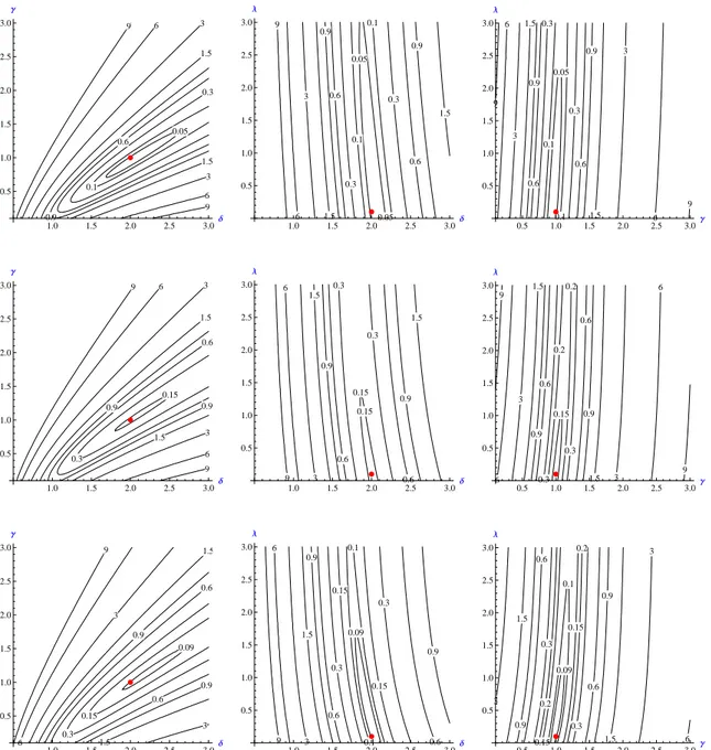
Figure 1: Contour plots of the objective function (6) for model (1) with X(t) following an IG − OU process with δ = 2, γ = 1, λ = 0.1. Length of series n = 1000. Row 1: univariate ch.f’s are used; Row 2: bivariate; Row 3: trivariate. Column 1: contour plots for (δ, γ); Column 2: contour plots for (δ, λ); Column 3: contour plots for (γ, λ). In all cases, the third parameter is set to its true value.
In this section we provide computational formulas and some simulation results on the important case of the Tempered Stable scenario for X(t).
From (17) we get
k0(ζ) = `k(ζ)
ζ = −2νδ
2ν(γ2+ 2ζ)ν−1. (18)
Using (18) in the last addend of (16), we note that the integral to be computed is of the form R
(1 + ceλs))ν−1ds; by appropriate transformations it can be given explicit form in terms of the hypergeometric function F (a, b, c, z) = Γ(c) Γ(a)Γ(b) ∞ X n=0 Γ(a + n)Γ(b + n) Γ(c + n) zn n!.
For details about convergence conditions and integral representations of this function we refer the reader to Abramowitz and Stegun (1972), pp. 556-558. In more detail for our case a solution can be obtained by Z (1 + ceλs)ν−1ds = 1 (ν − 1)λ µ 1 + e−λs/c 1 + ceλs ¶1−ν F (1 − ν, 1 − ν, 2 − ν, −e−λs/c).
When ν = 1/2 one obtains the IG stochastic volatility model. This case can be considerably simplified; in particular, we report below the cumulant function of S1, . . . , Sm for m = 1. Letting
AT denote the ArcTanh function and tj− tj−1 = ∆, we have
log(E(eiζSj)) = 2δ ³ ζ2 2 − iζβ ´ · AT µ (B−1) q 1 +2(1−e−λ∆γ)(ζ2λ2/2−iζβ) ¶ − AT (B−1) ¸ λγB , where B = q
1 +2(ζ2/2−iζβ)γ2λ . As we see, although cumbersome, the above function is
straightfor-wardly applicable in numerical procedures.
When m > 1, the ch.f. of S1, . . . , Sm can be obtained by means of (14). Note that the last
integral in (16) is given by Z tl tl−1 c1(l)k0 ³ c1(l) + c2(l, m)eλs ´ ds = −δc1(l) Z tl tl−1 (γ2+ 2(c1(l) + c2(l, m)eλs))−1/2ds,
whose explicit solution is equal to −δc1(l) Ã −2AT Ã (γ2+ 2c 1(l) + 2c2(l, m)eλs)1/2 (γ2+ 2c1(l))1/2 ! Á λ(γ2+ 2c1(l))1/2 ¯ ¯ ¯ ¯ tl tl−1 ! .
Here we give a brief report on some results with simulated data by estimating the parameters for model (1) with µ = β = 0 and where X(t) follows an IG(δ, γ) OU process with δ = 2, γ = 1 and auto-regression parameter λ = 0.1. We generated a series of observations of length 1000 of the volatility process X(t) as described in Taufer and Leonenko (2009) and successively used it in a Euler scheme to generate S. Figure 1 depicts the contour plots of the objective function. Each row indicates use of the m-variate ch.f., m = 1, 2, 3; each colums shows a possible pair of the three target parameters.
Although this example is based on a single series, the results are quite promising, also in the light of the little time used in the minimizing procedure. Inspection of the contour plots reveals quite a regular behavior of the objective function, with very low values in the neighborhood of the true parameter values.
4
Numerical results
The preceding sections provide an analysis of the most relevant results and open problems concerning ch.f.-based estimation of non-Gaussian OU processes. There is in particular one issue that requires further investigation. We have discussed consistency and asymptotic normality of the estimators; however, no information is available about the rate of convergence of the estimators, so that the actual validity of these results in finite samples has to be investigated numerically. In this and the next section we limit ourselves to the case of the Inverse Gaussian distribution. We first consider the case m = 2, p = 1 (no superposition) and then extend the analysis to the case m = 2, p = 2, corresponding to the superposition of two OU processes.
As pointed out in section 2.1, finding the optimal weighting function W (·) in (6) is not trivial in a framework like the present one, where the observations are not i.i.d. As no general solution is available (Jiang and Knight 2002, pag. 206), we will adopt a strategy that has frequently been used in applications and has proved to have reasonable properties in similar frameworks, namely an exponentially decreasing weight function.
4.1 Simulation experiment 1: no-superposition
The results of the no-superposition case are shown in Table 1 and Figure 2. At each replication we simulate the process with T = 1500 and discard the first 500 observations, in order to eliminate the effect of the starting point. Then we minimize the objective function (6); the integral is computed numerically by means of the R function adapt, based on the algorithm developed by Berntsen et
al. (1991). The minimization is performed by the R function constrOptim, which employs the
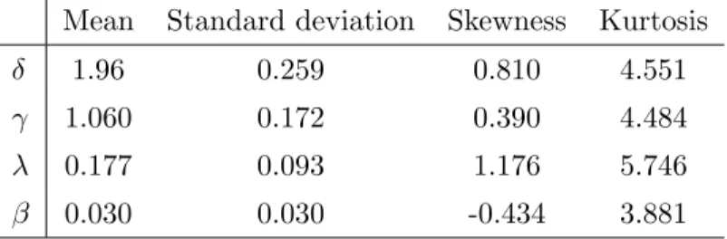
Nelder-Mead simplex method. Because of the heavy computational burden we limit ourselves to the simulation of B = 100 replications of the process (1) with X(t) given by (2). The values of the parameters used to simulate the process are δ = 2, γ = 1, λ = 0.1 and β = 0.03. Table 1 shows the sample mean, standard deviation, skewness and kurtosis computed across the 100 replications. Figure 2 displays the simulated distributions of the estimators.
Table 1: Simulation results with p = 1 (true values: δ = 2, γ = 1, λ = 0.1, β = 0.03). Mean Standard deviation Skewness Kurtosis
δ 1.96 0.259 0.810 4.551
γ 1.060 0.172 0.390 4.484
λ 0.177 0.093 1.176 5.746
β 0.030 0.030 -0.434 3.881
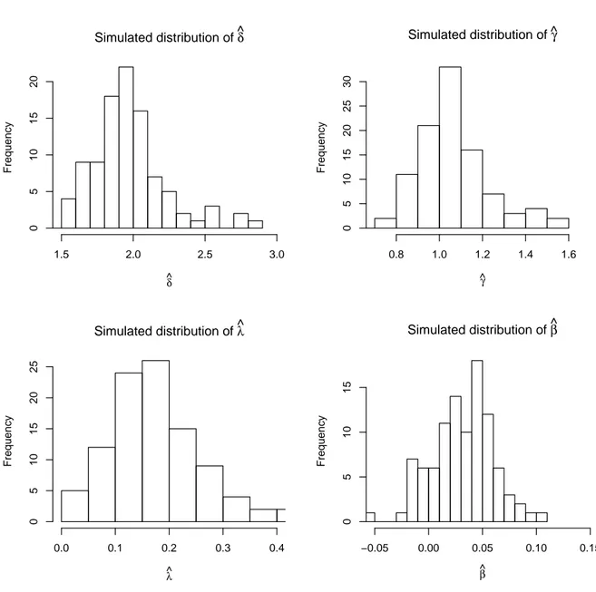
Despite the small number of replications, the results are quite interesting. In particular, the estimators seem to be approximately unbiased and the simulated distributions are bell-shaped.
Simulated distribution of δ^ δ ^ Frequency 1.5 2.0 2.5 3.0 0 5 10 15 20 Simulated distribution of γ^ γ ^ Frequency 0.8 1.0 1.2 1.4 1.6 0 5 10 15 20 25 30 Simulated distribution of λ^ λ^ Frequency 0.0 0.1 0.2 0.3 0.4 0 5 10 15 20 25 Simulated distribution of β^ β ^ Frequency −0.05 0.00 0.05 0.10 0.15 0 5 10 15
4.2 Simulation experiment 2: superposition of two OU processes
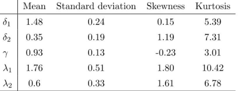
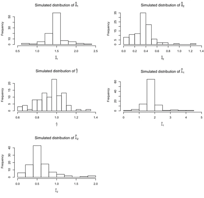
The simulation performed in the preceding subsection is repeated here when X(t) is the sum of 2 independent OU processes (see (4)). The remaining settings of the experiment are the same as before, with the exception of the parameter β, which is now set to zero. Results are shown in Table 2 and Figure 3.
Table 2: Simulation results with p = 2 (true values: δ1= 1.5, δ1= 0.5, γ = 1, λ1= 1.5, λ2 = 0.5).
Mean Standard deviation Skewness Kurtosis
δ1 1.48 0.24 0.15 5.39
δ2 0.35 0.19 1.19 7.31
γ 0.93 0.13 -0.23 3.01
λ1 1.76 0.51 1.80 10.42
λ2 0.6 0.33 1.61 6.78
The results are comparable to the case p = 1, with just a small loss of precision due to the larger number of parameters. Only the estimators of λ1 and λ2 seem to be less stable than the estimator
of λ in the no-superposition setup: the standard deviation of ˆλ1 is more than five times larger than
the standard deviation when p = 1.
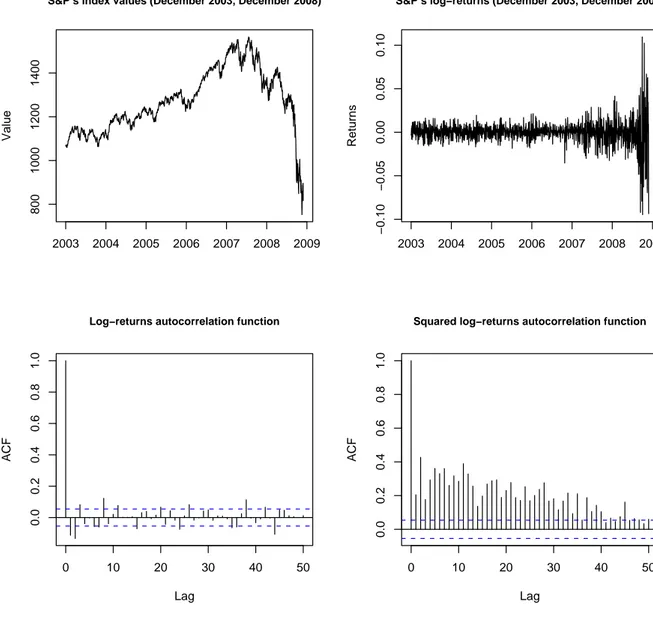
4.3 A real-data application: the S&P’s 500 volatility
In this subsection we fit model (1) to the daily log-prices of the Standard & Poor’s index over the 5-years period from December 1, 2003 to December 1, 2008. We consider either the case where the volatility process X(t) is a single Inverse-Gaussian OU process (p = 1) and the case where it is the superposition of two indepedent Inverse-Gaussian OU processes (p = 2). The first two panels of figure 4 display respectively the time series of levels and of log-returns; the remaining two panels show the autocorrelation function of the returns and of the squared returns.
Simulated distribution of δ^1 δ ^ 1 Frequency 0.5 1.0 1.5 2.0 2.5 0 10 30 50 Simulated distribution of δ^2 δ ^ 2 Frequency 0.0 0.2 0.4 0.6 0.8 1.0 1.2 1.4 0 5 15 25 35 Simulated distribution of ^γ γ ^ Frequency 0.6 0.8 1.0 1.2 1.4 0 5 10 15 20 Simulated distribution of λ^1 λ ^ 1 Frequency 0 1 2 3 4 5 0 20 40 60 Simulated distribution of λ^2 λ ^ 2 Frequency 0.0 0.5 1.0 1.5 2.0 0 10 20 30 40
S&P’s index values (December 2003, December 2008) Value 2003 2004 2005 2006 2007 2008 2009 800 1000 1200 1400
S&P’s log−returns (December 2003, December 2008)
Returns 2003 2004 2005 2006 2007 2008 2009 −0.10 −0.05 0.00 0.05 0.10 0 10 20 30 40 50 0.0 0.2 0.4 0.6 0.8 1.0 Lag ACF
Log−returns autocorrelation function
0 10 20 30 40 50 0.0 0.2 0.4 0.6 0.8 1.0 Lag ACF
Squared log−returns autocorrelation function
Table 3 reports some basic descriptive statistics. Most well-known stylized facts typically ob-served in financial data are evident: in particular, there are clusters of volatility and the data are strongly leptokurtic. Some other features of the data are strictly related to the downward trend of the last three months, caused by the financial crisis that took place in the second half of the year 2008. There is little evidence of autocorrelation of the log-returns series, with a couple of negative values at lags 1 and 2; on the contrary, the squared log-returns are strongly correlated, with significant values approximately up to lag 40. In addition, the negative skewness is probably a consequence of the large negative returns often observed in the last three months of the series.
Table 3: Basic descriptive statistics
Mean Standard deviation Skewness Kurtosis -0.0002 0.0129 -0.4672 20.8052
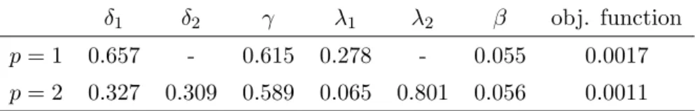
Estimation of parameters was performed as in sections 4.1 and 4.2 with bivariate ch.fs and an exponentially decreasing weight function. Table 4 shows the estimates and the value of the objective function (6) at convergence obtained when implementing model (1) respectively with p = 1 and p = 2 superpositions.
Table 4: Estimation results
δ1 δ2 γ λ1 λ2 β obj. function
p = 1 0.657 - 0.615 0.278 - 0.055 0.0017
p = 2 0.327 0.309 0.589 0.065 0.801 0.056 0.0011
The most relevant difference observed when moving from p = 1 to p = 2 concerns the parameters of the volatility processes, namely λ1 and λ2. It can indeed be seen that λ2 is much larger than
λ, whereas λ1 is very small. A plausible interpretation is that the two processes of the case p = 2
λ) and to large, rare and persistent shocks (the process with smaller λ). Analogous results about
these parameters were obtained by Griffin and Steel (2006, p. 627). When p = 1, an intermediate value of λ is obtained because a single process has to account for all the movements. Note that since the sum of δ1 and δ2 in the case p = 2 is approximately equal to δ1 when p = 1 and γ is
nearly unchanged, the marginal distribution of the volatility remains essentially the same for the two models. The risk-premium coefficient β is positive in both cases, as expected from financial theory; its relatively large value is in line with the high level of risk in the period considered in the present application.
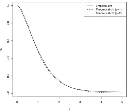
With the aim of evaluating the goodness-of-fit in the cases p = 1 and p = 2, we now compare the theoretical ch.fs and autocorrelation functions of the estimated processes with their empirical counterparties.
Consider first the ch.fs. Figure 5 shows three functions: each of them is the sum of the squares of the real and imaginary parts of a ch.f.. The first one (solid line) is the empirical ch.f.; the second one (dashed line) is the estimated ch.f. with p = 1; the third one (dotted line) is the same function with p = 2. In all of these cases we let ζ1 vary in the interval [0, 5] and fix ζ2 = 0. The two estimated
functions are virtually indistinguishable and in good agreement with the empirical ch.f. This seems to suggest that the marginal distribution is estimated quite precisely and that the approach works well for either value of p.
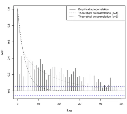
Next we turn to the dependence structure of the processes: especially when the squared log-returns exhibit a strong autocorrelation, the analysis of the autocorrelation of the observed and estimated processes is an important measure of goodness-of-fit. Notice that the theoretical autocor-relation function of the squared log-returns can be obtained using the results in Barndorff-Nielsen and Shephard (2001a, sect. 4.2). In this case the evidence is quite different. Figure 6 shows the
0 1 2 3 4 5 0.0 0.2 0.4 0.6 0.8 1.0 ζ chf Empirical chf Theoretical chf (p=1) Theoretical chf (p=2)
0 10 20 30 40 50 0.0 0.2 0.4 0.6 0.8 1.0 Lag ACF
Squared log−returns autocorrelation function
Empirical autocorrelation Theoretical autocorrelation (p=1) Theoretical autocorrelation (p=2)
theoretical autocorrelation functions of the estimated processes for p = 1 and p = 2: for comparison purposes, we also reported the empirical autocorrelation function of the observed squared returns. It is clear that with p = 2 the autocorrelation function decreases much more slowly and therefore captures more precisely the autocorrelation in the data. This allows to conclude that adding a second component improves considerably the fit to the dependence structure of the returns, while, as seen above, the marginal distribution is estimated approximately in the same way by the two models.
5
Conclusions
In this paper we have considered the problem of estimating the parameters of a continuous-time stochastic volatility model where the latent volatility follows an OU process. These processes are well suited for modelling some typical stylized facts observed in financial data. However, their estimation is quite difficult because usually the likelihood function cannot be written in closed form. Here we have developed an estimation method that makes use of the ch.f.; this technique is quite appealing because it is aymptotically equivalent to maximum likelihood.
The main contribution of the paper consists in extending some results first given by Barndorff-Nielsen and Shephard (2001a) in order to obtain the explicit expression of the ch.f. for various choices of the marginal distribution of the volatility process. We have investigated, by means of some simulation experiments, the small sample behavior of the estimators. Finally the method has been applied to the estimation of the volatility process of the daily time series of the S&P’s 500 equity index over the period 2003-2008.
From a theoretical point of view the method proposed in this article is convenient because it avoids both discretization and simulation. The results of the Monte Carlo experiments confirmed
the validity of the approach. As for the real-data analysis, the autocorrelation function of the squared log-returns decays very slowly. In accordance to other previous studies, in this case the superposition of two OU processes provides a better fit than a single OU process, allowing to estimate more precisely the dependence structure of the process.
A possible extension of these models is via the use of continuous superpositions where one could also introduce long-memory in the volatility process (see Barndorrf-Nielsen and Lenenko (2005) for details). The technique of estimation adopted here seems feasible in these cases even though it may be difficult to obtain explicit expressions; instead one would be able to get expressions for cumulants and the approach the problem of estimation by means of GMM.
References
Abramowitz, M. and Stegun, I.A. (1972). Handbook of mathematical functions, 10th printing. Applied Mathematics Series - 55, National Bureau of Standards, Washington, D.C..
Anh, V.V., Heyde, C.C., Leonenko, N.N. (2002). Dynamic models of long-memory processes driven by L´evy noise. J. Appl. Probab. 39, 730–747.
Barndorff-Nielsen, O.E. and Shephard, N. (2001a). Non-Gaussian Ornstein-Uhlenbeck-based models and some of their uses in financial economics. J. R. Stat. Soc. Ser. B Stat. Methodol. 63, 167-241. Barndorff-Nielsen, O.E. and Shephard, N. (2001b). Modelling by L´evy processes for financial econo-metrics. In Barndorff-Nielsen, O.E., Mikosch, T. and Resnick, S.I., L´evy processes. Theory and
applications, Birkh¨auser, Boston, MA, 283-318.
Barndorff-Nielsen, O.E. and Shephard, N. (2002). Econometric analysis of realized volatility and its use in estimating stochastic volatility models. J. R. Stat. Soc. Ser. B Stat. Methodol. 64, 253-280. Barndorff-Nielsen, O.E. and Shephard, N. (2003). Integrated OU processes and non-Gaussian
OU-based stochastic volatility models. Scand. J. Stat. 30, 277-295.
Barndorff-Nielsen, O.E. and Leonenko, N.N. (2005). Spectral properties of superpositions of Ornstein-Uhlenbeck type processes. Methodol. Comput. Appl. Probab. 7, 335-352.
Berntsen, J., Espelid, T.O. and Genz, A. (1991). An Adaptive Algorithm for the Approximate Calculation of Multiple Integrals. ACM Trans. Math. Softw. 17, 452-456.
Black, F. and Scholes, M. (1973). The pricing of options and corporate liabilities. Journal of
Political Economy 81, 637-654.
Cont, R. (2001). Empirical properties of asset returns: stylized facts and statistical issues. Quant.
Finance 1, 223-236.
Epps, T.W. (2005). Tests for location-scale families based on the empirical characteristic function,
Metrika 62, 99-114.
Feuerverger, A. (1990). An efficiency result for the empirical characteristic function in stationary time-series models. Canad. J. Statist. 18, 155-161.
Feuerverger, A. and McDunnough, P. (1981). On some fourier methods for inference. J. Amer.
Stat. Assoc. 76, 379-387.
Gander, M.P.S. and Stephens, D.A. (2007a). Stochastic volatility modelling in continuous time with general marginal distributions: inference, prediction and model selection. J. Stat. Plann. and Infer. 137, 3068-3081.
Gander, M.P.S. and Stephens, D.A. (2007b). Simulation and inference for stochastic volatility models driven by L´evy processes. Biometrika 94, no. 3, 627-646.
Griffin, J.E. and Steel, M.F.J. (2006). Inference with non-Gaussian Ornstein-Uhlenbeck processes for stochastic volatility. J. Econometrics 134, 605-644.
Jiang, G.J. and Knight, J.L. (2002). Estimation of continuous-time processes via the empirical characteristic function. J. Bus. Econom. Statist. 20, 198-212.
Jongbloed, G. and van der Meulen, F.H. (2006). Parametric estimation for subordinators and induced OU processes. Scand. J. Statist. 33, 825-847.
Jongbloed, G., van der Meulen, F.H. and van der Vaart, A.W. (2005). Nonparametric inference for L´evy-driven Ornstein-Uhlenbeck processes. Bernoulli, 11, 759-791.
Knight, J.L. and Yu, J. (2002). Empirical characteristic function in time series estimation.
Econo-metric Theory, 18, 691-721.
Knight, J.L., Satchell, S.E. and Yu, J. (2002). Estimation of the stochastic volatility model by the empirical characteristic function method. Aust. N. Z. J. Stat., 44, 319-335.
Leonenko, N.N., Taufer, E. (2005). Convergence of integrated superpositions of Ornstein Uhlenbeck processes to fractional Brownian motion. Stochastics: An International Journal of Probability and
Stochastic Processes 77, 477-499.
Madan, D.B. and Seneta, E. (1987). Simulation of estimates using the empirical characteristic function International Statistical Review 55, 153-161.
Merton, R. (1973) Theory of Rational Option Pricing. Bell Journal of Economics and Management
Science 4, 141-183.
Roberts, G.O., Papaspiliopoulos, O. and Dellaportas, P. (2004). Bayesian inference for non-Gaussian Ornstein-Uhlenbeck stochastic volatility processes. J. R. Stat. Soc. Ser. B Stat. Methodol., 66, 369-393.
Schoutens, W. (2003). L´evy Processes in Finance. Wiley, Chichester.
function. J. Econometrics 102, 111-141.
Sørensen, M. (2000). Prediction based estimating functions. Econometrics J., 3, 123-147.
Taufer, E. and Leonenko, N.N. (2009). Simulation of L´evy-driven Ornstein-Uhlenbeck processes with given marginal distribution. Computational Statistics and Data Analysis 53, 2427-2437. Taufer, E. and Leonenko, N.N. (2009). Characteristic function estimation of non-Gaussian Ornstein-Uhlenbeck processes. J. Stat. Plann. Infer., in press.
Todorov, V. and Tauchen, G. (2006). Simulation methods for L´evy-driven continuous-time autore-gressive moving average (CARMA) stochastic volatility models. J. Bus. Econom. Statist., 24, 455-469.
Woerner, J.H.C. (2007). Inference in L´evy-type stochastic volatility models. Adv. Appl. Prob. 39, 531-549.
Yu, J. (2004). Empirical characteristic function estimation and its applications. Econometric Rev. 23, 93-123.