https://doi.org/10.1051/0004-6361/201834003 c ESO 2019
Astronomy
&
Astrophysics
A ring in a shell: the large-scale 6D structure
of the Vela OB2 complex
?
,
??
T. Cantat-Gaudin
1, M. Mapelli
2,3, L. Balaguer-Núñez
1, C. Jordi
1, G. Sacco
4, and A. Vallenari
31 Institut de Ciències del Cosmos, Universitat de Barcelona (IEEC-UB), Martí i Franquès 1, 08028 Barcelona, Spain e-mail: [email protected]
2 Institut für Astro- und Teilchenphysik, Universität Innsbruck, Technikerstrasse 25/8, 6020 Innsbruck, Austria 3 INAF, Osservatorio Astronomico di Padova, vicolo Osservatorio 5, 35122 Padova, Italy
4 INAF, Osservatorio Astrofisico di Arcetri, Largo E. Fermi 5, 50125 Florence, Italy Received 1 August 2018/ Accepted 2 November 2018
ABSTRACT
Context. The Vela OB2 association is a group of ∼10 Myr stars exhibiting a complex spatial and kinematic substructure. The all-sky GaiaDR2 catalogue contains proper motions, parallaxes (a proxy for distance), and photometry that allow us to separate the various components of Vela OB2.
Aims. We characterise the distribution of the Vela OB2 stars on a large spatial scale, and study its internal kinematics and dynamic history.
Methods. We make use of Gaia DR2 astrometry and published Gaia-ESO Survey data. We apply an unsupervised classification algorithm to determine groups of stars with common proper motions and parallaxes.
Results. We find that the association is made up of a number of small groups, with a total current mass over 2330 M . The three-dimensional distribution of these young stars trace the edge of the gas and dust structure known as the IRAS Vela Shell across ∼180 pc and shows clear signs of expansion.
Conclusions. We propose a common history for Vela OB2 and the IRAS Vela Shell. The event that caused the expansion of the shell happened before the Vela OB2 stars formed, imprinted the expansion in the gas the stars formed from, and most likely triggered star formation.
Key words. stars: pre-main sequence – ISM: individual objects: IRAS Vela Shell – ISM: individual objects: Gum Nebula – ISM: bubbles – open clusters and associations: individual: Vela OB2
1. Introduction
The Vela OB2 region is an association of young stars near the border between the Vela and Puppis constellations, first reported by Kapteyn (1914). The association was known for decades as a sparse group of a dozen early-type stars (Blaauw 1946; Brandt et al. 1971; Straka 1973). The modern defini-tion of the Vela OB2 associadefini-tion comes from the study of de Zeeuw et al. (1999), who used Hipparcos parallaxes and proper motions to identify a coherent group of 93 members. Their positions on the sky overlaps with the IRAS Vela Shell (Sahu 1992), a cavity of relatively low gas and dust density, itself located in the southern region of the large Gum nebula (Gum 1952).
The Vela OB2 association is known to host the massive binary system γ2Vel, made up of a Wolf-Rayet (WR) and an
O-type star; recent interferometric distance estimates have located it at 336+8−7pc (North et al. 2007).De Marco & Schmutz(1999) estimate the total mass of the system to be 29.5 ± 15.9 M , while
Eldridge (2009) propose initial masses of 35 M and 31.5 M
? The movie associated to Fig. 6 is available at https://www.
aanda.org
?? Selected young stars from photometry and their membership probability are only available at the CDS via anonymous ftp to
cdsarc.u-strasbg.fr (130.79.128.5) or via http://cdsarc. u-strasbg.fr/viz-bin/qcat?J/A+A/621/A115
for the WR and O components, respectively.Pozzo et al.(2000), making use of X-ray observations, identified a group of pre-main sequence (PMS) stars around γ2 Vel, 350–400 pc from us. This
association is often referred to as the Gamma Velorum clus-ter, although Dias et al.(2002) list it under the name Pozzo 1. Jeffries et al.(2009) estimate that this cluster is 10 Myr old. The Gaia-ESO Survey study ofJeffries et al. (2014; hereafter J14) made use of spectroscopic observations to select the young stars on the basis of their Li abundances, and found the Gamma Velo-rum cluster to present a bimodal distribution in radial velocity. They suggested one group (population A) might be related to γ2Vel, while the other (population B) is not, and is in a
super-virial state. The N-body simulations ofMapelli et al.(2015) con-firmed that given the small total mass of the Gamma Velorum cluster, the observed radial velocities could only be explained if both components were supervirial and expanding. In a study of the nearby 30 Myr cluster NGC 2547,Sacco et al. (2015; here-after S15) identified stars whose radial velocities matched that of population B of J14, 2◦south of γ2Vel, hinting that this
asso-ciation of young stars might be very extended.Prisinzano et al. (2016) estimate a total mass of the Gamma Velorum cluster of about 100 M , which is a very low total mass for a group
con-taining a system as massive as γ2 Vel. As pointed out by J14, and according to the scaling relations ofWeidner et al.(2010), the total initial mass of a cluster should be at least 800 M in
Fig. 1.Left panel: spatial distribution of Gaia DR2 sources with parallaxes in the range 1.8 < $ < 3.4 mas. The black dots indicate known OCs in the area and distance range. We indicate the areas surveyed by dZ99 (de Zeeuw et al. 1999), D17 (Damiani et al. 2017), and B18 (Beccari et al. 2018). Top middle panel: α vs. $. Top right panel: proper motion diagram for the same sources, indicating the mean proper motion of the known OCs (taken fromCantat-Gaudin et al. 2018a). The dashed box indicates our initial proper motion selection. Red and blue points respectively indicate populations A and B fromJeffries et al.(2014). Bottom right panel: colour-magnitude diagram of the stars that fall in the proper motion box defined in top right panel.
It has been suggested (e.g.Sushch et al. 2011) that the IRAS Vela Shell (IVS) is a stellar-wind bubble created by the most mas-sive of the Vela OB2 stars. Observations of cometary globules (Sridharan 1992;Sahu et al. 1993;Rajagopal & Srinivasan 1998) and gas (Testori et al. 2006) have shown that the IVS is currently in expansion at a velocity of 8−13 km s−1.Testori et al.(2006)
point out that stellar winds from all the known O and B stars in the area are probably not sufficient to explain this expansion, and suggest it could have been initiated by a supernova, pos-sibly the one from which the runaway B-type star HD 64760 (HIP 38518) originated (Hoogerwerf et al. 2001). We note that Choudhury & Bhatt(2009) do not measure a significant expan-sion of the cometary globule distribution, but do observe that the tails of the 30 globules all point away from the centre of the IVS. Based on Gaia DR1 data,Damiani et al.(2017) have shown the presence of at least two dynamically distinct populations in the area. One of this groups includes the Gamma Velorum cluster, while the other includes NGC 2547. Still using Gaia DR1 data, Armstrong et al.(2018) found that the young stars in the region are distributed in several groups and do not all cluster around γ2Vel. Recently,Franciosini et al.(2018) have used the
astromet-ric parameters of the Gaia DR2 catalogue (Gaia Collaboration 2018) to confirm that populations A and B identified by J14 are located ∼38 pc from each other along our line of sight, and observe a radial velocity gradient with distance which they interpret as a sign of expansion. The Gaia DR2 catalogue was also used by Beccari et al.(2018), who find that the stars of the age of Gamma Velorum in a 10◦× 5◦field are not distributed in only two sub-groups, but in at least four different subgroups.
In this study we use Gaia DR2 data to characterise the spatial distribution and kinematics of stars of the age of the Vela OB2 association. This paper is organised as follows. Section 2 presents the data and our source selection. Section 3 contains
a description of the observed spatial distribution. Section 4 discusses the mass content in the Vela OB2 complex. Section5 relates our findings to the context of the IVS. Sections 6 dis-cusses the results. Concluding remarks are presented in Sect.7.
2. Data and target selection
We obtained data from the Gaia DR2 archive1 on a larger area
than previous studies (∼30◦ × 30◦) and in the parallax range
1.8 < $ < 3.4 mas, including the Gamma Velorum complex and nearby clusters. We follow the recommendations given in Eqs. (1) and (2) of Arenou et al.(2018) to keep sources with good astrometric solutions. The spatial distribution and proper motions of these stars are shown in Fig.1, along with the foot-print of the areas covered by previous studies. We also indi-cate the positions and mean astrometric parameters of the nearby OCs, taken fromCantat-Gaudin et al.(2018a). In order to retain the stars related to the Gamma Velorum cluster, we first apply broad proper motion cuts, then perform a photometric selection.
2.1. Proper motion pre-selection
Without any kind of selection beyond the applied quality fil-ters and parallax cuts, the proper motion diagram of the region (Fig. 1, top right panel) already shows a significant level of substructure, with two main groups corresponding to the two kinematical populations identified byDamiani et al.(2017). We exclude a priori the known nearby OCs that are older than the stars of the Gamma Velorum cluster (see HR diagrams in Fig.A.1) by only keeping the stars with −8 < µα∗< −3 mas yr−1
and 5 < µδ < 12 mas yr−1. We include BH 23 in this selection, 1 https://gea.esac.esa.int/archive/
Fig. 2.Left panel: HR diagram of the stars selected from their proper motions (see Fig.1), showing our photometric selection. The dashed line is a PARSEC isochrone of age 10 Myr (solar metallicity, AV = 0.35). Red and blue points respectively indicate populations A and B from Jeffries et al. (2014). Right panel: spatial distribution of the selected stars.
whose age and proper motion suggest it could be related to the Vela OB2 stars (also mentioned byConrad et al. 2017), although it is located 50 pc further away than Gamma Velorum.
2.2. Photometric selection
We then performed a photometric selection meant to separate the clearly visible PMS seen in the bottom right panel of Fig.1. The shape of the applied cuts and the resulting spatial distribution of these stars are shown in Fig.2. The dashed line in Fig.2is a PARSEC isochrone (Bressan et al. 2012) using the Gaia pass-bands derived by Evans et al.(2018). The choice of isochrone parameters (10 Myr, solar metallicity, AV= 0.35) is not the result
of a best fit, but simply highlights the expected path of the PMS in the HR diagram. The lower edge of the filter roughly follows a 30 Myr isochrone, and is intended to remove the PMS stars of the age of NGC 2547 or older. We verify in Fig. B.1 that our photometric selection produces the desired effect. We note that after performing the photometric selection, the remaining stellar distribution does not extend beyond α ∼ 130◦and further south than δ ∼ −55◦, but extends almost 15◦north of γ2Vel.
2.3. Cleaning the sample
We applied the unsupervised classification code UPMASK (Krone-Martins & Moitinho 2014). The approach does not assume a structure or distribution in spatial or astrometric space, but requires that sources with similar astrometry are more tightly distributed in (α,δ) than a uniformly random distribution. The tightness of the distribution is estimated through the total length of the minimum spanning tree (MST) connecting the selected sources, which we require to be shorter than the mean MST of random distributions by at least 3-σ. The procedure is repeated 100 times, each time shuffling the data within the nominal uncer-tainties. For each source, the frequency p (ranging from 0% to 100%) with which it is classified as a part of a clustered group can be interpreted as a membership probability, or a quantifica-tion of the coherence between astrometric ($, µα∗, µδ) and
spa-tial distribution (α, δ). We refer toCantat-Gaudin et al.(2018b) for an application of UPMASK to astrometric data.
The advantage of this approach is that we do not require clus-ters to be locally dense, but simply that they occupy an area smaller than the total field of view, allowing extended or elon-gated structures to be retained if they are made up of stars with consistent proper motions and parallaxes. The approach is also
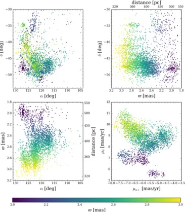
Fig. 3.All panels use the same colour-coding by parallax. Top left panel: distribution of the stars retained as probable members (p > 50%) of the Vela OB2 complex. Top right panel: $ vs. δ for the same stars. Bottom left panel: α vs. $. Bottom right panel: proper motions.
independent of the number of clusters present in the data, as it only discards the sources that do not appear to belong to any clus-ter. The distribution of sources with p > 50% is shown in Fig.3. Although UPMASK does not rely on assumptions on the spatial distribution of sources (e.g. by fixing a scale or requir-ing that clusters are centrally concentrated), the procedure still requires the user to arbitrarily define a threshold for the statisti-cal significance of the identified groups, here set to 3-σ. We note that the loose group seen around (α, δ)= (109◦,−34◦) in Fig.2
shows a large dispersion in proper motions and parallax, and therefore is not classified as significantly clustered by our pro-cedure. These stars could be the remnant of a rapidly expanding group. The list of stars selected from photometry and the values pwe computed are available at the CDS.
3. A fragmented spatial and kinematic distribution The stars coeval with the Gamma Velorum cluster are distributed over a large area, with some clearly visible compact clumps (shown in top row of Fig.4). Each of these components exhibits a distinct parallax and proper motion. We arbitrarily label in Fig.4 those that appear more prominent. Most of them can be easily distinguished from their location on the sky, but the groups we labelled A, B, C, and D appear continuous and partially over-lap in positional space and in astrometric space. We disentan-gled their position in astrometric space by modelling their (µα∗, µδ, $) distribution with a mixture of four covariant Gaussians.
One could arbitrarily define more groupings as individ-ual components, for instance along the bridge of stars con-necting our components A and G. The locations and mean astrometric parameters (and associated standard deviations) of the 11 components we define are listed in Table1. Their proper
Fig. 4.Top panels: spatial distribution of stars in three different parallax ranges, with contour levels showing local surface density in a 0.5◦ radius. Bottom panels: length and orientation of arrows indicate the mean tangential velocity (with respect to the main component A) in a 0.5◦
radius, if at least five stars are present within this radius.
motions are shown in Fig. 5. The proper motion distribution appears continuous for components H, G, A, B, C, and F, but some of the other groups we define exhibit distinct proper motions, in particular the three most distant groups I, J, and K. The HR diagrams of each component are shown in Fig.B.1.
In our final sample, half the stars have fractional parallax errors under 3%, and 96% have fractional errors under 10%. Such small fractional errors allow us to directly estimate distances with the approximation that d ' $1. The Gaia DR2 parallaxes are affected by a small negative zero-point offset of about 0.03 mas (Arenou et al. 2018), which for our sources is smaller than the typical nominal uncertainty. Local biases also exist, possibly reaching 0.1 mas (Lindegren et al. 2018), which corresponds to a ∼30 pc bias for the most distant stars in our sample, and to ∼10 pc for the most nearby. Figure6offers a representation of the three-dimensional stellar density distribution, obtained converting the individual parallaxes of each star to distances.
We converted the proper motion of each source to a tan-gential velocity2 and plot the velocity relative to the mean of
2 v t' 4.74
µ
$with µ in mas yr−1, $ in mas, vtin km s−1.
component A in the bottom row of Fig. 4. We note that the velocity field is far from homogeneous.
Following the choice of J14, we label the Gamma Velorum cluster (surrounding γ2Vel) component A. The compact
group-ing of a dozen stars located 1◦north of γ2Vel and labelled
clus-ter 5 byBeccari et al.(2018) shares similar proper motions with A, and does not appear as a distinct clump in the density map of Fig.4due to our choice of smoothing length. The mean parallax $ = 2.86 mas is close to the value of $ = 2.895 mas quoted by Franciosini et al.(2018), who focused on the stars identified as members of A by J14.
The clump we label B corresponds to the group B of J14, although we note that some of the stars observed by J14 belong to a third population we call C (cluster 2 ofBeccari et al. 2018), located 3◦ to the south-west of γ2 Vel. In Fig. 5 (second,
third, and fourth panels) we show that the J14 B stars exhibit bimodality in proper motion, parallax, and radial velocity. The J14 B stars with the larger radial velocities also tend to occupy the south of the field investigated by J14. We therefore consider that B and C are distinct objects with RV dispersions of 0.84 and 0.90 km s−1(respectively), rather than one single group with
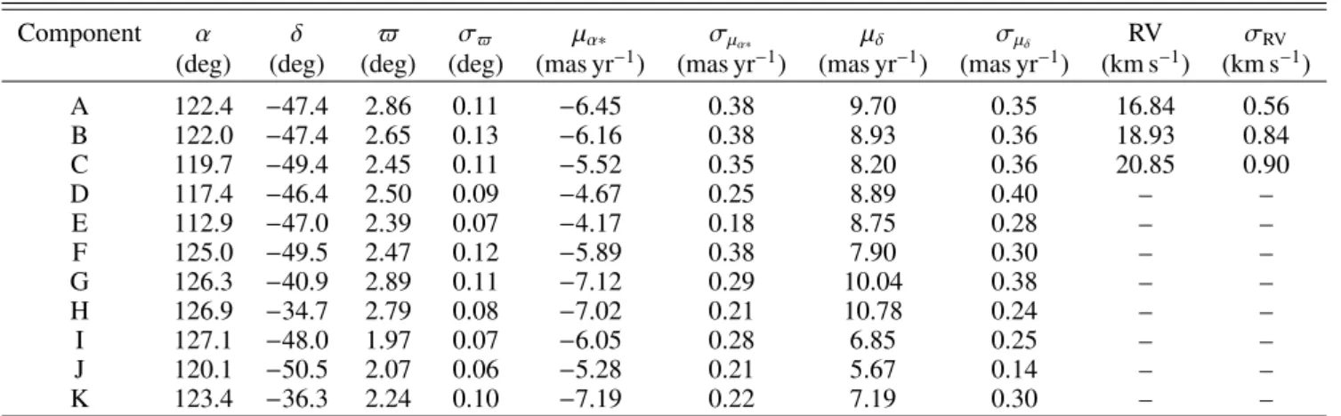
Table 1. Mean parameters of the main components identified in Fig.4.
Component α δ $ σ$ µα∗ σµα∗ µδ σµδ RV σRV
(deg) (deg) (deg) (deg) (mas yr−1) (mas yr−1) (mas yr−1) (mas yr−1) (km s−1) (km s−1)
A 122.4 −47.4 2.86 0.11 −6.45 0.38 9.70 0.35 16.84 0.56 B 122.0 −47.4 2.65 0.13 −6.16 0.38 8.93 0.36 18.93 0.84 C 119.7 −49.4 2.45 0.11 −5.52 0.35 8.20 0.36 20.85 0.90 D 117.4 −46.4 2.50 0.09 −4.67 0.25 8.89 0.40 – – E 112.9 −47.0 2.39 0.07 −4.17 0.18 8.75 0.28 – – F 125.0 −49.5 2.47 0.12 −5.89 0.38 7.90 0.30 – – G 126.3 −40.9 2.89 0.11 −7.12 0.29 10.04 0.38 – – H 126.9 −34.7 2.79 0.08 −7.02 0.21 10.78 0.24 – – I 127.1 −48.0 1.97 0.07 −6.05 0.28 6.85 0.25 – – J 120.1 −50.5 2.07 0.06 −5.28 0.21 5.67 0.14 – – K 123.4 −36.3 2.24 0.10 −7.19 0.22 7.19 0.30 – –
Notes. The radial velocity RV is the median of the combined radial velocities from J14 and S15. The associated standard deviation σRV is 1.4826× the median absolute deviation (MAD).
Fig. 5.Top left panel: ellipses represent the mean and standard deviation of proper motions of the main components (as defined in Fig.4). Top right panel: proper motions of the stars belonging to population A and B of J14Jeffries et al.(2014; red and blue, respectively) and population B ofSacco et al.(2015; yellow). Bottom left panel: proper motions of all stars with radial velocities in J14 and S15, colour-coded by radial velocity. Bottom right panel: same as previous panel, colour-coded by Gaia DR2 parallax.
a dispersion of 1.60 km s−1 (as reported by J14). In Fig. 5 we
can see that the stars identified by S15 as probable members of Gamma Velorum B belong to this population C. The group we label F can also be found in the southern part of the region, and has similar proper motions to C.
The most massive clump after A is the one we label D. Its location matches the group labelled Escorial 25 by
Caballero & Dinis(2008) in their study of OB association with Hipparcos data. This group also corresponds to cluster 1 of Beccari et al. (2018), and is visible in the PMS distribution map byArmstrong et al.(2018). Its tangential velocity in the α direction is larger than the velocity of A, meaning it is reducing its angular distance to A (see bottom middle panel of Fig.4). Unfortunately, without an estimate of the radial velocity of this
Fig. 6.Isosurfaces of the 3D density distributions of the stars shown in Fig.3. The distribution was smoothed with a Gaussian kernel of radius 2 pc. The lower density level shown is 0.5 stars pc−3. Distance from us roughly increases from left to right. The α, δ, and distance arrows cor-respond to physical dimensions of 20 pc. Components E and J are too sparse to be visible with the adopted contour levels, and component F is behind A and B from this vantage point. The animated figure is availableonline.
group of stars, we cannot determine whether its path will cross with other components of the association. Further west lies a small compact group we label E, with a similar tangential velocity to D.
We note a distribution of stars extending from A to the north, itself fragmented, with two major components we label G and H. The velocity distribution along this branch appears to vary continuously (see bottom left panel of Fig. 4), with clump G moving away from A, and clump H at the extreme north of this branch moving away from G.
In the background, we identify three groups with parallaxes smaller than 2.3 mas. They also exhibit significantly different velocities from the rest of the association. A loose branch of stars is visible linking components I and K (top right and bot-tom right panels of Fig. 4). The stars in this structure also share a common velocity and are consistently moving west-wards (with respect to component A). Component J, on the far southern border of the region under study, exhibits a distinct southward velocity. The HR diagrams shown in Fig.B.1 sug-gest that components I and K are slightly older than the rest of the Vela OB2 association (but younger than NGC 2547 and the other young OCs present in the area). We note that component K contains the known OC BH 23 (which we included in our initial proper motion selection, as mentioned in Sect.2.1), and appears to match the group labelled Escorial 27 in Caballero & Dinis (2008).
4. Mass distribution in the complex
Jeffries et al. (2014) and Prisinzano et al. (2016) have pointed out that the presence of such a massive system as γ2 Vel (over 30 M ) is puzzling in a cluster that does not seem to
contain more than ∼100 M . According to the empirical
scal-ing relations of Weidner et al. (2010), clusters hosting such a massive star typically contain a total mass of at least 800 M .
Fig. 7.Top row: spatial distributions of stars in three different abso-lute magnitude ranges. Bottom panel: normalised cumulative distribu-tion of the local density (number of neighbours within a fixed radius) for the 72 high-mass stars (blue) and 2120 low-mass stars (red). The grey curves correspond to 200 random re-drawings of 72 points from the total sample.
The results presented in this study show that the current total mass of the Vela OB2 complex is much higher than previously thought.
We performed a simple estimation based on the PARSEC isochrone featured in Fig.2(10 Myr, AV= 0.35, solar
metallic-ity), and converted the observed (GBP− GRP) colours to masses.
Summing up all the individual masses of the stars we consider astrometric members of the association (p > 50%), we obtain a total mass of 2330 M . The total mass content is likely higher if
the low-mass stars are included as this calculation only includes the stars we could identify as probable members, which are all brighter than MG= 10.5 (corresponding to 0.2 M ).
We studied the possible difference in spatial distribution between the high-mass and low-mass stars in the complex (shown in the top panel of Fig.7). We quantified mass segrega-tion using the approach ofAllison et al.(2009), who determine the length of a minimal spanning tree (MST) connecting the brightest stars, and compares it to the MST of a random realisa-tion of the total sample. We also followed the recommendarealisa-tions of Parker et al.(2011) andMaschberger & Clarke(2011), who use moving windows containing fixed numbers of stars. None of these diagnostics was able to reveal a significant level of mass segregation.
We also attempted to quantify whether the massive stars are preferentially distributed in areas that are also occupied by low-mass stars. In this case our results are at odds with those obtained byArmstrong et al.(2018), who observe that the mas-sive stars in their sample do not follow the same spatial distri-bution as the less massive ones. We performed a similar test to theirs, comparing the local density (considering all stars in the sample) around high-mass and low-mass stars. The cumula-tive distributions shown in Fig.7 are essentially identical, with a Kolmogorov–Smirnov test p-value of 0.65. The distribution of the 72 most massive stars is therefore compatible with a random sample of any 72 Vela OB2 stars. We observe that 14% of the
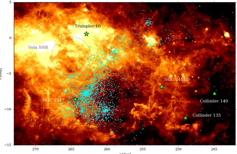
Fig. 8.60 µm map from the Improved Reprocessing of the IRAS Survey (IRIS,Miville-Deschênes & Lagache 2005), in Galactic coordinates. The cyan dots are the Vela OB2 stars identified in this study. The Vela SNR and the five older OCs located in the region are also indicated.
high-mass stars have no neighbour within 0.25◦ (against only
9% of the low-mass stars).
Although we cannot explain the discrepancies observed by Armstrong et al.(2018) and this study, we note the following:
– out of the 82 OB stars considered members of Vela OB2 by de Zeeuw et al.(1999), only 61 are present in the Gaia DR2 catalogue, due to the bright magnitude limit of Gaia; – out of these 61 stars, 20 have Gaia DR2 proper motions
incompatible with them being members of the Vela OB2 complex as defined in this study;
– photometric selections of PMS stars are able to produce purer samples than selections of OB stars, which cannot dis-criminate between stars of different ages.
We therefore conclude that in our sample, the high-mass and low-mass samples do not present statistically distinct distributions.
5. The large-scale structure and the IRAS Vela shell The region studied in this paper is located within the Gum nebula (Gum 1952), which has an apparent diameter of more than 30◦(e.g.Chanot & Sivan 1983). Its origin is still debated,
although most authors suggest that the nebula is likely an old supernova remnant (Woermann et al. 2001;Purcell et al. 2015). The Gum nebula is located about 500 pc from us, straddles the plane of the Milky Way (extending from l ∼ −15◦ to l ∼ +15◦), and our line of sight in its direction overlaps with
a number of different objects (Fig.8). The Vela Molecular Ridge contains a string of HII regions at distances of 800 pc–2 kpc Rodgers et al.(1960),May et al.(1988),Pettersson & Reipurth (1994),Neckel & Staude(1995),Prisinzano et al.(2018), which are not related to the Vela OB2 complex. They are visible as bright compact regions in Fig.8, roughly constrained to |b| < 2◦. About 10◦ to the north-west of γ2 Vel lies the Vela supernova
remnant (Vela SNR), one of the closest SNRs to us (250 ± 30, Cha et al. 1999), deploying an apparent diameter of 8◦. Dis-tance estimates from VLBI parallax place its central pulsar at 287+19−17pc (Dodson et al. 2003).
The most relevant structure to our study is the IRAS Vela Shell (IVS). Discovered as a ring-like structure in IRAS (Neugebauer et al. 1984) far-infrared images by Sahu (1992), and with a proposed radius of ∼65 pc, the IVS appears to be a substructure located near the front face of the Gum neb-ula. Although not recognised as a distinct structure at the time, the IVS can in fact be seen in the dark cloud maps of Feitzinger & Stuewe (1984; see also Pereyra & Magalhães 2002), and traced by the distribution of cometary globules (Zealey 1979;Zealey et al. 1983;Reipurth 1983). It is also vis-ible in maps of interstellar extinction (Franco 2012).Sridharan (1992) have suggested that the cometary globule ring bordering the IVS is expanding, a result supported by Sahu et al.(1993) and Rajagopal & Srinivasan (1998).Testori et al. (2006) show that a gas counterpart to the dust IVS exists, and exhibits signs of expansion.Sushch et al.(2011) propose a model for the structure of the complex that includes the Vela SNR and the IVS. They
suggest that the IVS is the result of the stellar-wind bubble of γ2Vel and the Vela OB2 association, and that the observed
asym-metry of the Vela SNR is due to the envelope of the Vela SNR physically meeting with the IVS. We note thatWoermann et al. (2001) proposed that the IVS might not be a separate entity, but rather the result of an anisotropic expansion of the Gum nebula.
In this study we find that the spatial distribution of the young stars in the Vela OB2 complex form a coherent, almost ring-like structure, a hint of which can be perceived in the top right panel of Fig.3 ($ vs. δ), and best visualised in Fig.6. The distance from clump A to K is 130 pc, which matches the early estimates ofSahu et al.(1993) for the diameter of the IVS, but the distance from H to I (the most distant clump from us) is 180 pc, indicating that the ring is not perfectly circular. The relative radial velocities of A, B, and C indicate that their distribution is stretching along our line of sight, as suggested byFranciosini et al.(2018). The relative tangential velocities of A, G, and H indicate that they are being pulled apart as well3. This behaviour, where all com-ponents are moving away from each other, is the signature of an expanding structure. We note that the far side of this ring is not as well-defined as the front side, and with the entire back half only traced by three clumps (I, J, and K) which exhibit slightly dif-ferent tangential velocities from the rest of the complex (Fig.4), and appear slightly older than the rest of the association as well (see Sect.3and Fig.B.1).
6. Discussion
The main conclusion of this paper is that the entire stellar dis-tribution of the Vela OB2 complex is expanding, which indi-cates that the expansion of the IVS is not due to stellar winds from the young OB stars, but caused by an event that took place before the Vela OB2 stars were formed, and imprinted the expanding motion into the stellar distribution itself. Their circular distribution hints at an episode of triggered star for-mation, caused by a mechanism energetic enough to not only compress gas into forming stars, but also induce the expansion of the IVS. Testori et al. (2006) have estimated that the total mechanical energy injected into the ISM by the joint action of the massive stars γ2Vel and ζ Pup and of the stellar aggregates
Trumpler 10 and Vela OB2 is insufficient by an order of magni-tude, and that supernovae might have driven this expansion. The presence of several ∼30 Myr OCs near the IVS (Collinder 135, Collinder 140, NGC 2451B, NGC 2547, Trumpler 10) makes this mechanism possible.
We propose the following scenario. About 20 Myr ago, the stars that now form the above-mentioned ∼30 Myr clusters were ∼10 Myr old, corresponding to the lifetime of a ∼15 M star.
Thus, we expect that the region was the site of intense super-nova activity, releasing enough energy to sweep gas out of the central cavity and to power the expansion of the IVS (e.g. Pelupessy & Portegies Zwart 2012). It is reasonable to expect that the expanding IVS produced a shock in the interstel-lar medium, which triggered a second burst of star formation approximately 10 Myr ago (e.g.Machida et al. 2005;Yasui et al. 2006). According to this scenario, γ2 Velorum and the other
∼10 Myr old stars were formed in this second burst of star
3 This expansion in the tangential plane is not a virtual effect due to our motion with respect to Vela OB2, as described in e.g.Brown et al.
(1997). If the perspective effect dominated, the positive radial velocity (∼18 km s−1) would induce a virtual contraction.
Fig. 9.Schematic picture of the proposed supernova-triggered star for-mation event. Stellar feedback and supernovae that exploded in the 30 Myr old clusters (yellow stars) swept the gas, producing the cen-tral cavity (white shell) and the IVS (blue shell). The expansion of the IVS triggered a second burst of star formation approximately 10 Myr ago (cyan stars).
formation. Their location approximately in the rim of the cavity confirms this interpretation. Figure9is a cartoon visualisation of this scenario.
The fact that the OCs in the region are ∼30 Myr old and approximately 20 Myr older than γ2 Velorum supports our
sce-nario, because the peak of core-collapse supernova activity occurs in the first 10−20 Myr and then it declines fast (see e.g. Fig. 1 ofMapelli & Bressan 2013). This age spread is also compatible with what is observed in numerical simulations of supernova-driven star formation (Padoan et al. 2016). No core-collapse supernovae are expected >50 Myr after cluster forma-tion.
Testori et al. (2006) mention that Hoogerwerf et al. (2001) identified a B-type runaway star (HD 64760, HIP 38518), and suggested it was ejected in a binary-supernova scenario that took place in the Vela OB2 region. The identification of hypervelocity stars from Gaia data (Renzo et al. 2018;Marchetti et al. 2019; Maíz Apellániz et al. 2018; Irrgang et al. 2018) might tell us whether other such objects are compatible with an origin inside the IVS. A full dynamical modelling of the orbits of hyperve-locity stars and nearby open clusters is beyond of the scope of this study, but should be possible based on the 3D velocities of these objects (Soubiran et al. 2018). The fact that Trumpler 10, NGC 2451B, Collinder 135, Collinder 140, and NGC 2547 all have very similar ages (see Fig.A.1) even suggests that they too might have originated from a single event of triggered star for-mation. The sparse group reported byBeccari et al.(2018) in the foreground of the region also shares a common age with these five clusters.
The supernova scenario also accounts for the slight age dif-ference between groups I, J, and K (as labelled in this study) and the rest of the Vela OB2 complex. If the gas distribution was not perfectly homogeneous at the time of the explosion, the com-pression wave caused by the supernova might have hit denser areas at the back of the bubble and initiate star formation there a few Myr before star formation took place in the front face of the shell. For a current diameter from 130 pc (the distance from A to
K, in agreement with the early estimate ofSahu et al. 1993) to 180 pc (the distance fro H to I), assuming the supernova event took place 10–20 Myr ago yields a constant expansion speed of the shell of 13–18 km s−1 (6.5 and 9 km s−1 with respect to the centre, respectively), in agreement with the 13 km s−1value
of Rajagopal & Srinivasan(1998) and with the 15.4 km s−1 of Testori et al.(2006).
In this study we did not attempt to characterise the dynam-ical state of each of the observed components. However, we have shown that the total mass of the structure is much larger than previously thought. We have also shown that the internal velocity dispersion of component B is smaller than the value of 1.6 km s−1 assumed by J14 and Mapelli et al. (2015). This smaller velocity dispersion in a deeper potential well indicates that B is not as supervirial as previously thought. A dedicated study of each component could determine whether any of them is going to survive as a bound cluster, or whether all of them will eventually disrupt. The typical expansion speed observed by Kuhn et al.(2019) in clusters younger than 5 Myr is ∼0.5 km s−1, corresponding to ∼0.5 pc Myr−1, which for a constant expansion rate leads to physical sizes of 5 pc after 10 Myr, matching the typical size of the observed components of Vela OB2.
The exact age of the Vela OB2 stars is still a debated issue; determinations from CMDs suggest an age between ∼7.5 Myr (Jeffries et al. 2017) and ∼10 Myr (Prisinzano et al. 2016), while lithium depletion measured from spectroscopy are compatible with an age of ∼20 Myr (Jeffries et al. 2017). The discrepancy between the ages of PMS stars obtained from lithium depletion patterns and from photometry has been noted in the literature (e.g.Bell et al. 2013, 2014;Messina et al. 2016; Bouvier et al. 2018). Our scenario relies on the age difference between the various populations rather than on their absolute age, and still holds if the photometric ages of the younger and older popu-lations are underestimated by a similar amount. The proposed scenario would only be invalid if the age difference turned out to be larger than ∼50 Myr, as the last core-collapse supernovae from the older population would have happened long before the formation of the younger population.
7. Conclusion
In this paper we make use of the Gaia DR2 astrometry and pho-tometry to identify the young stars of the Vela OB2 association over more than 100 pc. We identify and list 11 main components of a fragmented distribution. They appear to roughly follow an expanding ring-like structure.
We observe a good morphological correlation between their three-dimensional distribution and kinematics and the dust and gas structure known as the IRAS Vela shell. The expanding stel-lar distribution indicates that the expansion of the shell is not pri-marily due to the Vela OB2 stars, but to an event that impacted the local dynamics before the Vela OB2 stars formed. This obser-vation is compatible with previous suggestions that the shell originates from a supernova explosion. The progenitor of this supernova might have belonged to one of the several clusters with ages ∼20 Myr older than Vela OB2 located in the region.
The lack of radial velocities for all stars in the association prevents us from painting a full three-dimensional dynamic por-trait of the region and its expansion. Robust age determinations and orbits for all the populations in the region are necessary in order to establish a physically plausible sequence of events and prove or disprove the hypothesis that the formation of the Vela OB2 stars was triggered by the supernova that initiated the expansion of the IRAS Vela shell.
Acknowledgements. TCG acknowledges support from the Juan de la Cierva – formación 2015 grant, MINECO (FEDER/UE). This work was supported by the MINECO (Spanish Ministry of Economy) through grant ESP2016-80079-C2-1-R (MINECO/FEDER, UE) and MDM-2014-0369 of ICCUB (Unidad de Excelencia “María de Maeztu”). MM acknowledges financial support from the MERAC Foundation, from INAF through PRIN-SKA, from MIUR through Progetto Premiale “FIGARO” and “MITiC”, and from the Austrian National Science Foundation through the FWF stand-alone grant P31154-N27. The prepa-ration of this work has made extensive use of Topcat (Taylor et al. 2005), and of NASA’s Astrophysics Data System Bibliographic Services, as well as the open-source Python packages Astropy (Astropy Collaboration 2013), numpy (Van Der Walt et al. 2011), scikit-learn (Pedregosa et al. 2011), and Mayavi (Ramachandran & Varoquaux 2011). The figures in this paper were produced with Matplotlib (Hunter 2007). This research has made use of Aladin sky atlas developed at CDS, Strasbourg Observatory, France (Bonnarel et al. 2000;
Boch et al. 2014). This work presents results from the European Space Agency (ESA) space mission Gaia. Gaia data are being processed by the Gaia Data Pro-cessing and Analysis Consortium (DPAC). Funding for the DPAC is provided by national institutions, in particular the institutions participating in the Gaia MultiLateral Agreement (MLA). The Gaia mission website ishttps://www. cosmos.esa.int/gaia. The Gaia archive website is https://archives. esac.esa.int/gaia.
References
Allison, R. J., Goodwin, S. P., Parker, R. J., et al. 2009,MNRAS, 395, 1449
Arenou, F., Luri, X., Babusiaux, C., et al. 2018,A&A, 616, A17
Armstrong, J. J., Wright, N. J., & Jeffries, R. D. 2018,MNRAS, 480, L121
Astropy Collaboration (Robitaille, T. P., et al.) 2013,A&A, 558, A33
Beccari, G., Boffin, H. M. J., Jerabkova, T., et al. 2018,MNRAS, 481, L11
Bell, C. P. M., Naylor, T., Mayne, N. J., Jeffries, R. D., & Littlefair, S. P. 2013,
MNRAS, 434, 806
Bell, C. P. M., Rees, J. M., Naylor, T., et al. 2014,MNRAS, 445, 3496
Blaauw, A. 1946, Publications of the Kapteyn Astronomical Laboratory Groningen, 52, 1
Boch, T., & Fernique, P. 2014, in Astronomical Data Analysis Software and Systems XXIII, eds. N. Manset, & P. Forshay,ASP Conf. Ser., 485, 277
Bonnarel, F., Fernique, P., Bienaymé, O., et al. 2000,A&AS, 143, 33
Bouvier, J., Barrado, D., Moraux, E., et al. 2018,A&A, 613, A63
Brandt, J. C., Stecher, T. P., Crawford, D. L., & Maran, S. P. 1971,ApJ, 163, L99
Bressan, A., Marigo, P., Girardi, L., et al. 2012,MNRAS, 427, 127
Brown, A. G. A., Dekker, G., & de Zeeuw, P. T. 1997,MNRAS, 285, 479
Caballero, J. A., & Dinis, L. 2008,Astron. Nachr., 329, 801
Cantat-Gaudin, T., Jordi, C., Vallenari, A., et al. 2018a,A&A, 618, A93
Cantat-Gaudin, T., Vallenari, A., Sordo, R., et al. 2018b,A&A, 615, A49
Cha, A. N., Sembach, K. R., & Danks, A. C. 1999,ApJ, 515, L25
Chanot, A., & Sivan, J. P. 1983,A&A, 121, 19
Choudhury, R., & Bhatt, H. C. 2009,MNRAS, 393, 959
Conrad, C., Scholz, R.-D., Kharchenko, N. V., et al. 2017,A&A, 600, A106
Damiani, F., Prisinzano, L., Jeffries, R. D., et al. 2017,A&A, 602, L1
De Marco, O., & Schmutz, W. 1999,A&A, 345, 163
de Zeeuw, P. T., Hoogerwerf, R., de Bruijne, J. H. J., Brown, A. G. A., & Blaauw, A. 1999,AJ, 117, 354
Dias, W. S., Alessi, B. S., Moitinho, A., & Lépine, J. R. D. 2002,A&A, 389, 871
Dodson, R., Legge, D., Reynolds, J. E., & McCulloch, P. M. 2003,ApJ, 596, 1137
Eldridge, J. J. 2009,MNRAS, 400, L20
Evans, D. W., Riello, M., De Angeli, F., et al. 2018,A&A, 616, A4
Feitzinger, J. V., & Stuewe, J. A. 1984,A&AS, 58, 365
Franciosini, E., Sacco, G. G., Jeffries, R. D., et al. 2018,A&A, 616, L12
Franco, G. A. P. 2012,A&A, 543, A39
Gaia Collaboration (Brown, A. G. A., et al.) 2018,A&A, 616, A1
Gum, C. S. 1952,The Observatory, 72, 151
Hoogerwerf, R., de Bruijne, J. H. J., & de Zeeuw, P. T. 2001,A&A, 365, 49
Hunter, J. D. 2007,Comput. Sci. Eng., 9, 90
Irrgang, A., Kreuzer, S., & Heber, U. 2018,A&A, 620, A48
Jeffries, R. D., Naylor, T., Walter, F. M., Pozzo, M. P., & Devey, C. R. 2009,
MNRAS, 393, 538
Jeffries, R. D., Jackson, R. J., Cottaar, M., et al. 2014,A&A, 563, A94
Jeffries, R. D., Jackson, R. J., Franciosini, E., et al. 2017,MNRAS, 464, 1456
Kapteyn, J. C. 1914,ApJ, 40
Krone-Martins, A., & Moitinho, A. 2014,A&A, 561, A57
Kuhn, M. A., Hillenbrand, L. A., Sills, A., Feigelson, E. D., & Getman, K. V. 2019,ApJ, 870, 32
Lindegren, L., Hernández, J., Bombrun, A., et al. 2018,A&A, 616, A2
Machida, M. N., Tomisaka, K., Nakamura, F., & Fujimoto, M. Y. 2005,ApJ, 622, 39
Maíz Apellániz, J., Pantaleoni González, M., Barbá, R. H., et al. 2018,A&A, 616, A149
Mapelli, M., & Bressan, A. 2013,MNRAS, 430, 3120
Mapelli, M., Vallenari, A., Jeffries, R. D., et al. 2015,A&A, 578, A35
Marchetti, T., Rossi, E. M., & Brown, A. G. A. 2019, MNRAS, in press, [arXiv:1804.10607]
Maschberger, T., & Clarke, C. J. 2011,MNRAS, 416, 541
May, J., Murphy, D. C., & Thaddeus, P. 1988,A&AS, 73, 51
Messina, S., Lanzafame, A. C., Feiden, G. A., et al. 2016,A&A, 596, A29
Miville-Deschênes, M.-A., & Lagache, G. 2005,ApJS, 157, 302
Neckel, T., & Staude, H. J. 1995,ApJ, 448, 832
Neugebauer, G., Habing, H. J., van Duinen, R., et al. 1984,ApJ, 278, L1
North, J. R., Tuthill, P. G., Tango, W. J., & Davis, J. 2007,MNRAS, 377, 415
Padoan, P., Pan, L., Haugbølle, T., & Nordlund, Å. 2016,ApJ, 822, 11
Parker, R. J., Bouvier, J., Goodwin, S. P., et al. 2011,MNRAS, 412, 2489
Pedregosa, F., Varoquaux, G., Gramfort, A., et al. 2011,J. Mach. Learn. Res., 12, 2825
Pelupessy, F. I., & Portegies Zwart, S. 2012,MNRAS, 420, 1503
Pereyra, A., & Magalhães, A. M. 2002,ApJS, 141, 469
Pettersson, B., & Reipurth, B. 1994,A&AS, 104, 233
Pozzo, M., Jeffries, R. D., Naylor, T., et al. 2000,MNRAS, 313, L23
Prisinzano, L., Damiani, F., Micela, G., et al. 2016,A&A, 589, A70
Prisinzano, L., Damiani, F., Guarcello, M. G., et al. 2018,A&A, 617, A63
Purcell, C. R., Gaensler, B. M., Sun, X. H., et al. 2015,ApJ, 804, 22
Rajagopal, J., & Srinivasan, G. 1998,JApA, 19, 79
Ramachandran, P., & Varoquaux, G. 2011,Comput. Sci. Eng., 13, 40
Reipurth, B. 1983,A&A, 117, 183
Renzo, M., Zapartas, E., & de Mink, S. E. 2018, ArXiv e-prints [arXiv:1804.09164]
Rodgers, A. W., Campbell, C. T., & Whiteoak, J. B. 1960,MNRAS, 121, 103
Sacco, G. G., Jeffries, R. D., Randich, S., et al. 2015,A&A, 574, L7
Sahu, M. S. 1992, PhD thesis, Kapteyn Institute, Postbus 800 9700 AV, Groningen, The Netherlands
Sahu, M., & Blaauw, A. 1993, Massive Stars: Their Lives in the Interstellar Medium, eds. J. P. Cassinelli, & E. B. Churchwell,ASP Conf. Ser., 35, 278
Soubiran, C., Cantat-Gaudin, T., Romero-Gomez, M., et al. 2018,A&A, 619, A155
Sridharan, T. K. 1992,JApA, 13, 217
Straka, W. C. 1973,ApJ, 180, 907
Sushch, I., Hnatyk, B., & Neronov, A. 2011,A&A, 525, A154
Taylor, M. B. 2005, in Astronomical Data Analysis Software and Systems XIV, eds. P. Shopbell, M. Britton, & R. Ebert,ASP Conf. Ser., 347, 29
Testori, J. C., Arnal, E. M., Morras, R., et al. 2006,A&A, 458, 163
Van Der Walt, S., Colbert, S. C., & Varoquaux, G. 2011,Comput. Sci. Eng., 13, 22
Weidner, C., Kroupa, P., & Bonnell, I. A. D. 2010,MNRAS, 401, 275
Woermann, B., Gaylard, M. J., & Otrupcek, R. 2001,MNRAS, 325, 1213
Yasui, C., Kobayashi, N., Tokunaga, A. T., Terada, H., & Saito, M. 2006,ApJ, 649, 753
Zealey, W. J. 1979,New Zealand J. Sci., 22, 549
Zealey, W. J., Ninkov, Z., Rice, E., Hartley, M., & Tritton, S. B. 1983,Astrophys. Lett., 23, 119
Appendix A: HR diagrams of nearby open clusters
Fig. A.1.HR diagrams of known OCs in the area of the Vela OB2 association. The membership was taken fromCantat-Gaudin et al.(2018a) and is based on astrometry only. The dashed and continuous lines correspond to PARSEC isochrones of 10 and 32 Myr, respectively; AV = 0.35; and solar metallicity.
Appendix B: HR diagrams of individual components
Fig. B.1.HR diagrams of the main identified components. Stars only compatible on the basis of their astrometry (black crosses); stars that also pass the photometric selection defined in Sect.2.2(blue dots). The dashed and continuous lines correspond to PARSEC isochrones of 10 and 32 Myr, respectively; AV = 0.35; and solar metallicity.