3040
|
wileyonlinelibrary.com/journal/mrm Magn Reson Med. 2020;84:3040–3053. F U L L PA P E RInvestigating the accuracy and precision of TE-dependent versus
multi-echo QSM using Laplacian-based methods at 3 T
Emma Biondetti
1,2|
Anita Karsa
2|
David L. Thomas
3,4|
Karin Shmueli
21Centre de NeuroImagerie de Recherche (CENIR) , Team “Movement Investigations and Therapeutics”, Institut du Cerveau (ICM), Inserm U 1127, CNRS
UMR 7225, Sorbonne Université, Paris, France
2Department of Medical Physics and Biomedical Engineering, University College London, London, United Kingdom 3Dementia Research Centre, UCL Queen Square Institute of Neurology, University College London, London, United Kingdom
4Wellcome Centre for Human Neuroimaging, UCL Queen Square Institute of Neurology, University College London, London, United Kingdom
This is an open access article under the terms of the Creative Commons Attribution License, which permits use, distribution and reproduction in any medium, provided the original work is properly cited.
© 2020 The Authors. Magnetic Resonance in Medicine published by Wiley Periodicals LLC on behalf of International Society for Magnetic Resonance in Medicine Correspondence
Emma Biondetti, Institut du Cerveau (ICM), Hôpital Pitié-Salpêtrière, 47 Boulevard de l’Hôpital, 75651 Paris Cedex 13, France.
Email: [email protected] Funding information
UCLH Biomedical Research Centre; UCL Leonard Wolfson Experimental Neurology Centre, Grant/Award Number: PR/ylr/18575; Engineering and Physical Sciences Research Council, Grant/Award Number: 1489882 and EP/L016478/1
Purpose: Multi-echo gradient-recalled echo acquisitions for QSM enable
optimiz-ing the SNR for several tissue types through multi-echo (TE) combination or in-vestigating temporal variations in the susceptibility (potentially reflecting tissue microstructure) by calculating one QSM image at each TE (TE-dependent QSM). In contrast with multi-echo QSM, applying Laplacian-based methods (LBMs) for phase unwrapping and background field removal to single TEs could introduce nonlinear temporal variations (independent of tissue microstructure) into the measured suscep-tibility. Here, we aimed to compare the effect of LBMs on the QSM susceptibilities in TE-dependent versus multi-echo QSM.
Methods: TE–dependent recalled echo data simulated in a numerical head
phan-tom and gradient-recalled echo images acquired at 3 T in 10 healthy volunteers. Several QSM pipelines were tested, including four distinct LBMs: sophisticated harmonic artifact reduction for phase data (SHARP), variable-radius sophisticated harmonic artifact reduction for phase data (V-SHARP), Laplacian boundary value background field removal (LBV), and one-step total generalized variation (TGV). Results from distinct pipelines were compared using visual inspection, summary statistics of susceptibility in deep gray matter/white matter/venous regions of in-terest, and, in the healthy volunteers, regional susceptibility bias analysis and non-parametric tests.
Results: Multi-echo versus TE-dependent QSM had higher regional accuracy,
especially in high-susceptibility regions and at shorter TEs. Everywhere except in the veins, a processing pipeline incorporating TGV provided the most tempo-rally stable TE-dependent QSM results with an accuracy similar to multi-echo QSM.
Conclusions: For TE-dependent QSM, carefully choosing LBMs can minimize the
1
|
INTRODUCTION
Quantitative susceptibility mapping aims to determine the underlying spatial distribution of tissue magnetic suscepti-bility (χ)1,2 from the phase (𝜙) of a gradient-recalled echo (GRE) MRI sequence:
where TE is the echo time; r is the voxel position in the image;
𝛾 is the proton gyromagnetic ratio; ΔBTot is the χ-induced total
field perturbation along the scanner’s z-axis; and 𝜙0 is a phase
offset at TE = 0.
Processing pipelines for QSM usually require unwrapping
𝜙 to resolve spatiotemporal 2𝜋 aliasing, removing background
field variations (ΔBBg) resulting from χ sources outside the
brain, and solving a local field (ΔBLoc)-to-χ ill-posed inverse
problem.2
Both single-echo and multi-echo GRE acquisitions can be used for QSM. Acquiring multiple TEs is advantageous primarily because the phase SNR (SNR(𝜙)) can be
opti-mized in multiple tissues simultaneously,1-3 as choosing TE = T∗2 for a tissue maximizes SNR(𝜙) in that tissue.1,4
Thus, combining multiple echoes via fitting or averaging over TEs results in a TE-independent field map designed to optimize SNR(𝜙) (see Equation 1). By acquiring
multi-echo GRE images and processing each TE separately, a method referred to as TE-dependent QSM,5 some studies5-7 have investigated the TE dependence of the QSM suscep-tibility resulting from nonlinear temporal variations of the phase. Acquiring multi-echo GRE images and combining all TEs improves the SNR of the resulting field map3,7 or QSM image1,7 compared to acquiring single-echo GRE images, but the regional accuracy and precision of χ cal-culated using TE-dependent versus multi-echo QSM has undergone limited investigation.
Regarding the accuracy of χ in TE-dependent QSM, χ measured using numerical simulations in a vein perpendic-ular to the external magnetic field was shown to be constant across a long range of TEs.1 However, χ measured using nu-merical simulations6 or real data5,6 was also shown to be TE-dependent, particularly at short TEs. In high-χ regions, such as microbleeds, such a TE dependence could arise from a fail-ure of Laplacian phase unwrapping to recover the true phase,6 or, motivated by the observation of a regional TE dependence of χ, it could be linked to intrinsic tissue properties.5,6
Regarding the precision of χ, simulated1,3 and in vivo data7 have shown that, for the range of TE values such that the measured MR signal is above the noise floor, single-echo χ noise decreases at longer TEs, combining multiple TEs by averaging over echoes reduces the propagation of phase noise into ΔBLoc compared with using single echoes3, and fitting an
increasing number of TEs progressively reduces the propaga-tion of phase noise into the multi-echo χ map compared with using single echoes.7
Processing pipelines for QSM often incorporate Laplacian-based methods (LBMs) for phase unwrapping8 or
ΔBBg removal.9 Laplacian phase unwrapping aims to identify
the unwrapped phase whose local derivatives are the most similar to the derivatives of the wrapped phase. Laplacian
ΔBBg removal aims to eliminate ΔBBg from the brain by
ex-ploiting their harmonicity (ie, ∇2(ΔB
Bg
)
= 0) inside the brain.
Because LBMs perform nonlinear operations, they must be applied carefully to avoid introducing inaccuracies into the processed signal phase. Notably, the effect on the accuracy and precision of χ using Laplacian-based phase unwrapping and ΔBBg removal in the same pipeline for multi-echo or
TE-dependent QSM has not been investigated. In fact, pre-vious studies on the noise in single-echo versus multi-echo QSM have not used LBMs1,7 or have used LBMs to perform
ΔBBg removal but not phase unwrapping.7 Moreover, they
have not compared the accuracy and precision of ΔBLoc and
χ calculated at each TE with the accuracy and precision of
ΔBLoc and χ calculated by combining all TEs.1,3,5-7
Because LBMs for phase unwrapping and ΔBBg removal
are frequently applied within the same QSM pipeline,5,6 it is important to systematically evaluate their effect on the accuracy and precision of TE-dependent versus multi-echo QSM. This could contribute to the standardization of image processing pipelines for TE-dependent QSM. Therefore, this study aimed to compare the effect of LBMs on the accuracy and precision of χ in TE-dependent versus multi-echo QSM. This was investigated using numerically simulated data and images acquired in vivo, incorporating LBMs for both phase unwrapping and ΔBBg removal into the QSM processing
pipelines.
2
|
METHODS
When not otherwise stated, image analysis was performed using MATLAB (R2017b; The MathWorks, Natick, MA) (1)
𝜙(r, TE) = 𝛾ΔBTot(r, TE) TE + 𝜙0(r)
K E Y W O R D S
magnetic resonance imaging, multi-echo QSM, quantitative susceptibility mapping, single-echo QSM, TE-dependent QSM
and statistical analysis was performed using Stata (R15; StataCorp, College Station, TX).
2.1
|
In vivo data acquisition
Multi-echo 3D GRE imaging of 10 healthy volunteers (av-erage age/age range: 26/22-30 years, 5 females) was per-formed on a 3 T system (Philips Achieva [Philips Medical Systems, Best, NL]; 32-channel head coil). A preliminary version of this study was presented at the 2017 meet-ing of the International Society for Magnetic Resonance in Medicine.10 All of the volunteers provided written in-formed consent, and the local research ethics committee approved the experimental sessions. Images were acquired using a transverse orientation (FOV = 240 × 240 × 144 mm3, isotropic voxel size = 1 mm3, flip angle = 20º, TR = 29 ms, five evenly spaced echoes [(TE1/TE spacing = 3/5.4 ms], bandwidth = 270 Hz/pixel, SENSE11 along the first/second phase-encoding directions = 2/1.5, flyback gradients along the frequency-encoding direction, and without flow-compensating gradients).
2.2
|
Data simulation from a numerical
head phantom
To ensure the availability of ground-truth χ values against which to test the accuracy of the QSM pipelines, a piece-wise constant Zubal numerical head phantom12 was used with a matrix size of 256 × 256 × 128 voxels3 and 1.5-mm isotropic voxel size and the following regions of interest (ROIs): four deep-gray matter ROIs (ie, the caudate nucleus [CN], globus pallidus [GP], putamen [PU], and thalamus [TH]), as QSM has often been used to study iron deposition in these regions4; one venous ROI in the superior sagittal sinus (SSS), as QSM can be used to investigate vein oxygenation in the healthy brain13,14 and in cerebrovascular disease15,16; and, to repre-sent the other main brain tissue types, cortical gray matter (GM), white matter (WM), and CSF ROIs were also included (see Supporting Information Figure S2). Based on this phan-tom, the ground-truth total field perturbation (ΔBTrue
Tot ) at 3T
MRI was simulated using a Fourier-based forward model.17 A noise-free multi-echo complex MRI signal C was
simu-lated throughout the brain using Equation 1 with ΔBTrue Tot and a
spatially variable 𝜙0 (see Supporting Information) as well as
a mono-exponential T∗2 magnitude signal decay:
where i is the unit imaginary number. To enable the compar-ison of in vivo results and numerical simulations, the TEs
in Equation 2 were matched to those of the in vivo 3D GRE protocol.
Random zero-mean Gaussian noise with a standard devi-ation (SD) equal to 0.07 was added to the real and imaginary parts of the noise-free signal independently.18 This value of SD was calculated by fulfilling the following high-SNR con-dition at the longest TE in the numerical phantom ROI with the shortest T∗2 (ie, the SSS19):
where A and 𝜎(A), respectively, denote the magnitude image
and its noise. Therefore, realistic noise affected the numerical simulations at all TEs and in all ROIs except the region outside the head, which was masked out during the QSM calculation.
2.3
|
Data preprocessing
A brain mask was calculated for each subject by applying the FSL Brain Extraction Tool (BET)20,21 with robust brain center estimation (threshold = 0.3) to the magnitude image at the longest TE. The mask was based on the longest TE, to account for the greater amount of signal loss (signal dropout near regions of high-susceptibility gradients) compared to shorter TEs.
A whole-brain mask for the Zubal phantom was calcu-lated by applying FSL BET20,21 with robust brain center es-timation (threshold = 0.05) to the T∗2 map of the numerical
phantom (see Supporting Information).
2.4
|
Processing pipelines for QSM
For TE-dependent QSM, the signal phase from each TE was processed separately. For multi-echo QSM, all of the pro-cessing pipelines received as an input the same total field map, which was calculated by nonlinearly fitting (NLFit) the complex multi-echo signal over TEs22 using the Cornell QSM software package’s Fit_ppm_complex function (http:// weill.corne ll.edu/mri/pages /qsm.html).
Three distinct processing pipelines incorporating LBMs for phase unwrapping and ΔBBg removal were implemented
as follows (Figure 1). The first processing pipeline ap-plied simultaneous phase unwrapping and ΔBBg removal
using SHARP (sophisticated harmonic artifact reduction for phase data), which is a direct solver of the discretized Poisson equation.23 SHARP was chosen because it has been widely used in the literature on QSM and has been shown to be both robust and numerically efficient.9 To minimize the number of voxels at the edge of the brain affected by convolution artifacts, SHARP was implemented using the (2)
C(r, TE) = A0(r) exp(− TE
T∗ 2(r)
)
exp (i𝜙 (r, TE))
(3)
A(SSS, TE5)
𝜎(A(SSS, TE5))
minimum-size 3-voxel isotropic 3D Laplacian kernel.23,24 SHARP was applied using a threshold for singular value decomposition equal to 0.05 and a brain mask with 2-voxel (numerical phantom) or 4-voxel erosion (healthy subjects). The threshold for singular value decomposition value used here was consistent with the values used in the original studies on SHARP23,24 and led to the best ΔB
Bg removal on
visual inspection.
Both the second and third processing pipelines first ap-plied Laplacian phase unwrapping with a threshold for singular value decomposition equal to 1-10 (ie, the default value in the Cornell QSM software package). Then, because larger kernel sizes have been shown to better recover small susceptibility variations, the second processing pipeline ap-plied SHARP with variable kernel size (V-SHARP)25 to the Laplacian-unwrapped phase with an initial kernel radius of approximately 7 mm and a 1-voxel step size/final kernel ra-dius. The third strategy applied the Laplacian boundary value (LBV) method26 to the Laplacian-unwrapped phase. The LBV was tested because, in a recent multicomparison study,9 it quantitatively outperformed all other methods for ΔBBg
re-moval. The Cornell QSM software package’s LBV function was used with default parameter values.
For TE-dependent QSM only, residual phase offsets were removed by applying V-SHARP with an initial kernel radius of approximately 40 mm and a 1-voxel step-size/final kernel radius.27
In all these pipelines, ΔBLoc-to-χ inversion was performed
using Tikhonov regularization2,28 with correction for suscep-tibility underestimation23 and using the L-curve method29 to determine the optimal value for the regularization parameter. This inversion method was chosen because it is computa-tionally efficient and has been shown to substantially reduce streaking artifacts relative to the truncated k-space division method.15 For each processing pipeline in the healthy volun-teers, the mean across subjects of the individually optimized Tikhonov regularization parameters was used.
Finally, to investigate a single-step processing pipeline in-corporating LBMs, a fourth processing pipeline using total generalized variation (TGV)30 was applied to the wrapped phase at each TE (TE-dependent QSM) or the NLFit field map (multi-echo QSM). The TGV method was chosen be-cause it has been shown to avoid stair-casing artifacts in the resulting QSM image while correctly preserving structural borders.30 It was implemented using Singularity (https:// github.com/CAIsr /qsm; Sylabs, Albany, CA) and the default FIGURE 1 Processing pipelines for TE-dependent and multi-echo QSM. For each Laplacian-based method (LBM) (SHARP [sophisticated harmonic artifact reduction for phase data], Laplacian boundary value [LBV], SHARP with variable kernel size [V-SHARP], and total generalized variation [TGV]), each input image (𝜙(TE1), 𝜙(TE2), 𝜙(TE3),𝜙(TE4),𝜙(TE5) and the combined total field map ΔBNLFit
Tot ) underwent exactly the same processing steps, following each processing stream described in the gray box
parameter values (𝛼1, 𝛼0)= (0.0015, 0.005) adopted in the
original TGV study based on the criterion that the 𝛼1:𝛼0= 3:1
ratio is optimal for medical imaging applications.30
2.5
|
Region-of-interest segmentation in the
healthy subject images
To enable the comparison of regional χ values between the simulated and in vivo data, ROIs similar to those defined in the numerical phantom were segmented in vivo (ie, the CN, GP, PU, TH, posterior corona radiata [PCR] as a WM ROI, and the straight sinus [StrS] as a venous ROI). We chose to consider the PCR instead of the whole WM, to minimize WM microstructural effects in the regional χ analysis, as WM microstructure was not modeled in the numerical phantom simulations. We chose to consider the StrS instead of the SSS as the venous ROI, because QSM calculation in vivo required larger amounts of brain mask erosion, which left only a few SSS voxels available for regional χ analysis.
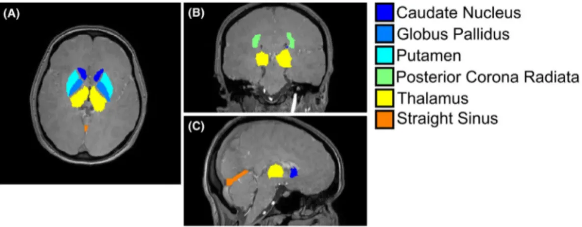
For each subject, the CN, GP, PU, TH, and PCR were seg-mented based on the Eve χ atlas31 (Figure 2), whose GRE magnitude image was aligned to each subject’s fifth-echo magnitude image using NiftyReg.32,33 The fifth-echo magni-tude image was chosen because it had the closest TE (24.6 ms) to that of the Eve GRE magnitude image (24 ms). Moreover, because the fifth-echo magnitude image had the best contrast between the StrS and the surrounding brain parenchyma, it was used to segment the StrS of each volunteer using the ITK-SNAP active contour segmentation tool34 (Figure 2).
2.6
|
Quantitative evaluation of the
measured χ
All of the processing pipelines (Figure 1) were applied to the noisy simulated images of the numerical phantom and
the images of the 10 healthy volunteers. To avoid combining effects induced by TE dependence or multi-echo combina-tion in a reference ROI with similar effects in the ROIs under investigation, the χ maps were not referenced (for example, to the CSF). Instead, it was assumed that ΔBBg removal
pro-vided sufficient χ referencing for the purpose of this study.9 In the numerical phantom simulations, the performance of each QSM pipeline relative to the ground truth was visually assessed by calculating a difference image between the corre-sponding χ map and 𝜒True. In the volunteers, because of the lack
of a ground truth, TE-dependent difference images were cal-culated relative to the corresponding multi-echo QSM image.
In the numerical phantom simulations, the means and SDs of χ were calculated for each pipeline in each phantom ROI with 𝜒 ≠0 (ie, the CN, GP, TH, PU, SSS, and WM)
(Supporting Information Figure S2). The root mean squared errors (RMSEs) of χ relative to 𝜒True were also calculated
throughout the brain volume as
where 𝜒̂ denotes the χ map calculated by the QSM pipeline, and ‖⋅‖2 is the Euclidean norm.
In the volunteers, the means and SDs of χ were calculated in each ROI and for each processing pipeline and compared against χ values in subjects of a similar age from the litera-ture. In the volunteers, RMSEs could not be calculated be-cause of the lack of a ground truth.
For visualization purposes in the volunteers, if pooling the regional means and SDs of χ across subjects was possible (ie, all intrasubject SDs of χ were larger than the intersubject SD of χ), the pooled χ averages (mp) and SDs (SDp) were
respec-tively calculated as (4) RMSE( ̂𝜒)�%�=‖ ̂𝜒(r)−𝜒True(r)‖2 ‖𝜒True(r)‖ 2 ⋅ 100 , (5) mp= ∑10 i=1nimi ∑10 i=1ni
FIGURE 2 Brain regions of interest (ROIs) in a representative volunteer. For a representative healthy subject, the ROIs segmented in the healthy volunteers are overlaid on a transverse (A), coronal (B), and sagittal (C) slice of the first-echo magnitude image
and
where mi and SDi respectively denote the individual mean and
SD of χ in the ith subject, and ni denotes the ROI size in voxels.
2.7
|
Statistical analysis
Statistical analyses were only performed on the volunteer data, because they required several distinct measurements for the average χ in each ROI.
The presence of a systematic bias in TE-dependent versus multi-echo QSM within the same processing pipeline (Figure 1) was investigated using Bland-Altman analysis of the average χ at each TE and for each ROI.
Statistically significant differences in multi-echo versus TE-dependent QSM within the same processing pipeline and ROI and at each TE were tested by considering the correspond-ing distributions of average χ values across subjects. To assess whether to apply parametric paired t-tests or nonparametric
sign tests, the normal distribution of the differences between paired χ values was assessed using the Shapiro-Wilk test.
3
|
RESULTS
3.1
|
Pooling of χ measurements
For each ROI and each processing pipeline, all intrasubject SDs of χ were larger than the intersubject SD; thus, mp and SDp were calculated according to Equations 5 and 6.
3.2
|
Performance of TE-dependent versus
multi-echo QSM
Here, only the results of the SHARP-based and TGV-based processing pipelines are presented, because these pipelines best estimated 𝜒True in the numerical phantom simulations.
The results of the V-SHARP-based and LBV-based process-ing pipelines are available in the Supportprocess-ing Information.
In the numerical phantom, Figures 3 and 4 show the multi-echo or TE-dependent susceptibility images (B-G and I-N) (6) SDp= �∑ 10 i=1(ni−1)SD2i �∑10 i=1ni � −10 ,
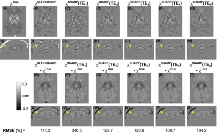
FIGURE 3 Echo time–dependent versus multi-echo susceptibility maps calculated using the SHARP-based processing pipelines. In the numerical phantom, the same transverse and sagittal slices are shown for the ground-truth susceptibility map (A,H), for the susceptibility map calculated using nonlinear fitting (NLFit) plus SHARP (B,I), and for the susceptibility maps calculated using the SHARP-based pipeline at each TE (C-G,J-N). The figure also shows the difference between each susceptibility map and the ground truth (O-Z). The bottom row shows the root mean squared errors (RMSEs) of χ. In all the sagittal images (H-N,U-Z), the yellow arrowheads point at the same location in the superior sagittal sinus (SSS)
calculated using the SHARP-based and TGV-based pipe-lines, their difference relative to the ground truth (O-Z), and the RMSEs of χ throughout the brain volume (bottom row). Figure 5 shows the means and SDs of χ calculated using the SHARP-based (A) or TGV-based pipelines (B) in each ROI. Analogous images for the V-SHARP-based and LBV-based pipelines are shown in Supporting Information Figures S4-S6.
For the numerical phantom simulations, the error between the calculated and ground-truth χ appeared fairly constant over TEs (Figures 3 and 4) except in some high-χ regions in which the error increased with TE (ie, the GP and SSS in the SHARP-based pipeline [Figure 5A] and the SSS only in the TGV-based pipeline [Figure 5B]).
The SSS, which was the highest χ structure (𝜒True =
0.3 ppm), showed the largest susceptibility errors for both SHARP-based and TGV-based TE-dependent QSM (Figure 5A,B). In the SHARP-based pipeline, large susceptibility errors were also observed in the GP, which was the sec-ond-highest χ structure (𝜒True = 0.19 ppm).
For one representative volunteer, Figures 6A-L and 7A-L show the multi-echo and TE-dependent susceptibility images respectively calculated using the SHARP-based and TGV-based pipelines. In addition, Figures 6M-V and
7M-V respectively show TE-wise differences between TE-dependent and multi-echo QSM. For each ROI in the healthy volunteers, Figure 5 shows the pooled means and SDs of multi-echo and TE-dependent χ calculated using the SHARP-based (C) or TGV-based pipelines (D). In the vol-unteers, susceptibility differences between TE-dependent and multi-echo QSM were most prominent in the StrS (ar-rowheads in Figures 6G-L,R-V and 7G-L,R-V) and at the shortest TEs.
In general, the average susceptibilities measured in the deep-GM ROIs and in the PCR (Figure 5C,D) had values within the ranges reported by previous studies25,31,35-38: 0.01-0.13 ppm for the CN, 0.06-0.29 ppm for the GP, 0.02-0.14 ppm for the PU, −0.02-0.08 ppm for the TH, and −0.06-0.03 ppm for the PCR. An exception was observed in the CN, in which the mean of 𝜒(TE1) was always smaller than the
correspond-ing minimum value reported in the literature (ie, 0.01 ppm). In the StrS, only the mean of the multi-echo χ calculated using the SHARP-based pipeline had a value close to the pre-viously reported range for venous blood, namely, 0.17-0.58 ppm13,15,37,39 (Figure 5C,D).
In both the numerical phantom simulations and the healthy volunteers, the QSM images appeared less noisy with FIGURE 4 Echo time–dependent versus multi-echo susceptibility maps calculated using the TGV-based processing pipelines. In the numerical phantom, the same transverse and sagittal slices are shown for the ground-truth susceptibility map (A,H), for the susceptibility map calculated using NLFit plus TGV (B,I), and for the susceptibility maps calculated using the TE-dependent TGV-based pipeline at each TE (C-G,J-N). The figure also shows the difference between each susceptibility map and the ground truth (O-Z). The bottom row shows the RMSEs of
increasing TE, as indicated by the susceptibility difference images (Figures 3O-Z, 4O-Z, 6M-V, and 7M-V). Finally, each TGV-based TE-dependent QSM image had larger RMSEs than the corresponding multi-echo QSM image (Figure 4, bottom row). A similar result was observed in the SHARP-based TE-dependent QSM images from the first to the third TE (Figure 3, bottom row).
3.3
|
Statistical analysis
In the healthy volunteers, for all processing pipelines and ROIs, the Shapiro-Wilk test rejected the hypothesis of nor-mally distributed paired differences of χ. Therefore, TE-dependent versus multi-echo QSM values were always evaluated using the nonparametric sign test.
For the SHARP-based and TGV-based processing pipe-lines, significant differences between TE-dependent and multi-echo QSM are highlighted in Figure 5C,D, whereas the bias between TE-dependent and multi-echo χ is shown in Figure 8. The same information for the V-SHARP-based and LBV-based pipelines is available in Supporting Information Figures S6C,D and S9. Biases smaller than |0.01| ppm (|⋅|
de-notes the absolute value) were considered negligible. For the SHARP-based processing pipeline, the bias of TE-dependent versus multi-echo χ was greater than |0.01| ppm in
the CN, GP, and StrS at all TEs (Figure 8A). For the TGV-based processing pipeline, the bias of TE-dependent versus multi-echo χ was greater than |0.01| ppm in the CN at TE1 and TE2, and in the StrS at all TEs (Figure 8B). In the CN for both processing pipelines and in the GP for the SHARP-based pipeline, the bias monotonically decreased with increasing FIGURE 5 The means and SDs (error bars) of χ are shown in each ROI of the numerically simulated (A,B) and pooled healthy volunteer data (C,D) for the TE-dependent and multi-echo SHARP-based and TGV-based processing pipelines for QSM. In the numerical phantom, the ground-truth χ is also shown. In the healthy volunteers, the TEs at which the TE-dependent χ differed significantly from the multi-echo χ are denoted using the symbol ★ (P-value < .05). Abbreviations: CN, caudate nucleus; GP, globus pallidus; PCR, posterior corona radiata; PU, putamen; StrS, straight sinus; TH, thalamus; WM, white matter
TEs, whereas in the StrS the bias decreased from the first to the third TE, then slightly increased again from the third to the fifth TE (Figure 8). In all the ROIs, the SD of the bias decreased with increasing TEs (Figure 8), reflecting the re-duced SD of χ at longer TEs (Figure 5C,D).
In general, the bias was greater than |0.01| ppm at the
same TEs at which there was a significant difference be-tween TE-dependent and multi-echo QSM (Figures 5C,D and 8).
4
|
DISCUSSION
This study aimed to compare processing pipelines for QSM that combine the GRE signal acquired at multiple TEs (multi-echo QSM) with those that process each TE individually (TE-dependent QSM) while applying four alternative strategies for Laplacian phase unwrapping and ΔBBg removal (Figure 1).
Multi-echo and TE-dependent QSM were compared by ap-plying each pipeline to data simulated using a head numerical phantom (Supporting Information Figures S1 and S2) and im-ages acquired in 10 healthy volunteers. The resulting χ values
depended on several factors. The first was the LBM used for
ΔBBg removal: simultaneous phase unwrapping and ΔBBg
re-moval using SHARP gave the most accurate multi-echo χ, and one-step TGV gave the most accurate TE-dependent χ, even at short TEs (Figure 5 and Supporting Information Figure S6). The second factor was the (ground-truth) χ of the ROI: larger reconstruction errors were observed in high-χ regions, such as the GP and the veins (Figure 5 and Supporting Information Figure S6). The third factor, for TE-dependent QSM only, was the TE: all pipelines except TGV gave less accurate χ val-ues than multi-echo QSM, especially at shorter TEs (Figure 5 and Supporting Information Figure S6).
In the numerical simulations, TE-dependent QSM always suffered greater susceptibility noise than multi-echo QSM in all ROIs except the veins (Figures 3-7). The imprecision of TE-dependent QSM was closely dependent on noise and de-creased with increasing TE (difference images in Figure 3 and SDs in Figure 5A,B). This finding is in line with previ-ously published results on noise in QSM over TEs,1,7 and, combined with the generally smaller RMSEs of multi-echo χ, suggests that multi-echo QSM offers the best processing pipeline performance across the whole brain.
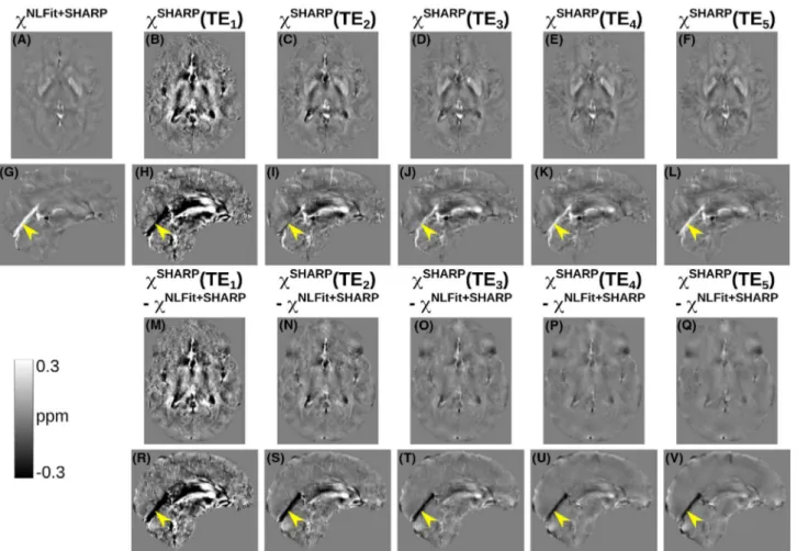
FIGURE 6 Echo time–dependent versus multi-echo χ maps in a representative healthy subject calculated using the SHARP-based processing pipelines. The same transverse and sagittal slices are shown for the susceptibility maps calculated using the SHARP-based multi-echo (A,G) and TE-dependent pipelines (B-F,H-L). The figure also shows the difference between each TE-dependent susceptibility map and the corresponding multi-echo image (M-V). In all the sagittal images (G-L,R-V), the yellow arrowheads point at the same location in the StrS
In the numerical phantom simulations, the accuracy of TE-dependent χ was similar at all TEs but decreased with increasing TE in the GP (𝜒SHARP) and the SSS (𝜒SHARP and
𝜒TGV) (Figure 5A,B). High-χ structures such as the SSS also
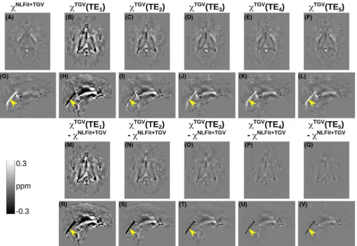
showed the largest χ errors in the difference images, where they were increasingly visible at longer TEs (arrows in FIGURE 7 Echo time–dependent versus multi-echo χ maps in a representative healthy subject calculated using the TGV-based processing pipelines. The same transverse and sagittal slices are shown for the susceptibility maps calculated using the TGV-based multi-echo (A,G) and TE-dependent pipelines (B-F,H-L). The figure also shows the difference between each TE-TE-dependent susceptibility map and the corresponding multi-echo image (M-V). In all the sagittal images (G-L,R-V), the yellow arrowheads point at the same location in the StrS
FIGURE 8 Bias of TE-dependent versus multi-echo QSM. The mean and SD (error bars) of the bias of TE-dependent versus multi-echo QSM are shown for the SHARP-based (A) and TGV-based (B) processing pipelines. In both bar plots, the gray band denotes the [−0.01- 0.01] ppm interval. If the mean of the bias was within this interval, the difference between the corresponding TE-dependent QSM pipeline and the multi-echo QSM pipeline was considered negligible
Figures 3U-Z and 4U-Z). This result is in line with previ-ous studies on simulated data,6 which suggest that this TE dependence can arise from the failure of Laplacian phase un-wrapping to accurately recover the true phase, especially in high χ regions. To address this limitation, future studies will investigate the application of alternative phase unwrapping methods.40
The numerical phantom used in this study was character-ized by an ROI-wise constant χ distribution. Therefore, in the numerical phantom simulations, an average χ close to 𝜒True
and a small SD of χ were positive indicators of a pipeline’s accuracy and precision, respectively. However, brain regions in vivo are characterized by a heterogeneous χ distribution within each ROI. Thus, without knowledge of the true SD of χ, a smaller SD does not necessarily indicate a pipeline’s greater precision in the healthy volunteers. For a compre-hensive evaluation of the effect of overregularization by particular pipelines, future work will involve implementing a numerical phantom with a known heterogeneous χ distribu-tion (SD) in each ROI.
In the healthy volunteers, in contrast with the numerical phantom simulations, the accuracy of TE-dependent QSM varied nonmonotonically over TEs (see the CN, PU, TH, and StrS in Figure 5C,D). As is discussed below, distinct factors could motivate this discrepancy in the deep GM and the ve-nous ROIs.
In the deep GM ROIs of healthy volunteers, the greater inaccuracy of shorter versus longer TEs (Figure 5C,D and Supporting Information Figure S6C,D) was possibly caused by additional tissue microstructure in vivo, which might cause a nonlinear temporal phase accumulation un-resolvable by conventional QSM algorithms.5,6 In partic-ular, short -T∗2 components at a subvoxel level, which are
preserved when using LBMs for phase unwrapping, could manifest as apparent nonlinearities at shorter TEs, thus explaining the TE dependence in the Laplacian-processed phase.6 Attempting to explain the TE dependence of in vivo QSM, previous studies5,6 have described the measured χ using multicompartment models, showing that three tissue compartments might accurately define the major χ sources in deep GM,5 and that a geometric model with axon, my-elin, and extra-axonal space microcompartments might ac-curately define the major χ sources in WM.41 However, in WM the TE dependence of phase41 was observed in fiber bundles with highly ordered microstructure, which was not the focus of our study.
In the StrS, the nonlinear variation of TE-dependent QSM and the lower accuracy of shorter versus longer TEs com-pared with the simulations could perhaps be explained by the lack of flow compensation in the acquisition sequence,42 which was a limitation of this study and particularly af-fected shorter TEs. As the maximum velocity of blood flow in healthy cerebral veins is about 25 cm/s, the maximum
displacement of spins flowing in the StrS at increas-ing TEs were estimated as x(TEi)= 250[mm∕s]⋅TEi[s]:
0.8, 2.1, 3.5, 4.8, and 6.2 mm. The exact encoded location of such flowing spins would depend on the StrS orienta-tion relative to the applied encoding gradients, and on the total phase accumulated by these spins at each TE. Over time, the zero-crossing points of the first moment of the frequency-encoding gradient were increasingly closer to the TE (Supporting Information Figure S3), indicating that the total phase accumulated by flowing spins along this en-coding direction would decrease over TEs. Therefore, the flow-induced χ error in the StrS would be expected to de-crease at increasing TEs. Instead, flow-induced artifacts did not appear prominent in the multi-echo χ maps (Figures 6G and 7G and Supporting Information Figures S7G and S8G), possibly because they were mitigated by the nonlinear fit-ting method used to combine multiple TEs.22 By assigning smaller weights to the phase at shorter TEs (at each TE, weights are inversely proportional to the level of noise in the phase), any flow-induced phase error or spatial shifts in the vessel location at the two shortest TEs were probably mitigated in the combined field map.
In the StrS, the greater discrepancy between multi-echo χ and TE-dependent χ at shorter TEs always resulted in a large χ estimation bias (Figure 8) corresponding to statistically sig-nificant differences between the two methods as measured by the sign test (Figure 5C,D). Although smaller, a bias corre-sponding to significant differences in the sign test was also found at longer TEs (Figures 5C,D and 8).
In ROIs other than the StrS, the difference between TGV-based TE-dependent and multi-echo QSM was only signif-icant at the first or second TEs (Figure 5D), whereas the difference between SHARP-based TE-dependent and multi-echo QSM was sometimes significant also at longer TEs (Figure 5C).
The results of the statistical analyses suggest that in 𝜒TGV
at shorter TEs, the estimation bias was mainly driven by the lower SNR of TE-dependent versus multi-echo QSM (larger limits of agreement at shorter TEs in Figure 5D). In 𝜒SHARP,
significant differences were sometimes found at longer TEs (see the CN, GP, and TH in Figure 5C), suggesting a potential underestimation of the true χ in addition to the lower SNR at shorter TEs. In both cases, unresolved tissue microstruc-ture components in the deep-GM ROIs and the lack of flow compensation in the StrS might have also contributed to the systematic bias between TE-dependent and multi-echo QSM.
In both the simulated and in vivo data, shorter-TE QSM images appeared noisier and were potentially affected by the fast decaying signal components linked to tissue microstruc-ture. Nonetheless, including all TEs always resulted in multi-echo QSM images with less noise or smaller RMSEs (in the numerical simulations) compared to excluding shorter TEs (Supporting Information Figures S10-S12).
The numerical phantom simulations did not include mod-eling of receive bandwidth–induced distortions along the fre-quency-encoding direction, as the effect of such distortions on the ROI-based χ calculation was found to be negligible in healthy volunteers. Indeed, here the largest bandwidth- induced distortions, calculated as the ratio between the unwrapped total field map and the pixel bandwidth,43 were lo-cated near the air–tissue interfaces and were within the [−1, 1] voxel range throughout the multi-echo field map.
In this study, all experiments were limited to one field strength (ie, 3 T). Although scanning at higher field strengths (eg, 7 T) would result in a higher phase at a given TE, this benefit may be counterbalanced by the decrease in T∗2 in
tis-sue compartments already subject to rapid decay at 3 T. Thus, even if nonlinearities in the phase over TEs have been ob-served at both 3 T6 and 7 T,5 further work is needed to assess the scalability of our results to ultrahigh fields.
Finally, it must be noted that in the numerical phantom simulations, all processing pipelines underestimated 𝜒True
(Figure 5A,B and Supporting Information Figure S6A,B). In QSM, some degree of underestimation is always expected, because the lack of MRI signal in the image background and zeros in the dipole kernel make the local field-to-susceptibil-ity problem ill-posed.2
5
|
CONCLUSIONS
For studies on the TE-dependent variation of χ, the LBMs in the QSM processing pipeline should be carefully chosen to minimize biasing the results with LBM-related temporal variations. To this aim, a processing pipeline based on one-step TGV could provide slightly more accurate results over different TEs compared with processing pipelines based on SHARP, V-SHARP or LBV, and thus enable a more accu-rate investigation of TE-dependent χ variations deriving from tissue microstructure. This does not necessarily apply to the quantification of χ in the WM. For maximum accuracy, WM χ should be modeled as a tensor rather than a scalar value, because of the ordered microstructure found in WM.41,44 Because there is no direct relationship between susceptibility tensor solutions and the single-orientation solution,45 our re-sults cannot directly inform on the accuracy and precision of tensor-based χ calculated from all the TEs versus single TEs of a multi-echo GRE protocol. Studies aimed at investigat-ing the TE-dependent evolution of χ in the veins should im-plement flow compensation to avoid different flow-induced phase contributions at different TEs. Finally, the observed nonlinearity in the signal phase at shorter TEs highlights the need for accurate modeling of short T∗2 tissue components.
Such modeling could also inform the design of more accurate digital brain phantoms, which is useful in methodological studies on TE-dependent QSM.
ACKNOWLEDGMENTS
E. Biondetti was supported by the UK Engineering and Physical Sciences Research Council (1489882). A. Karsa was supported by the EPSRC-funded UCL Centre for Doctoral Training in Medical Imaging (EP/L016478/1) and the Department of Health’s National Institute for Health Research–funded Biomedical Research Centre at University College London Hospitals. D.L. Thomas was supported by the UCL Leonard Wolfson Experimental Neurology Centre (PR/ylr/18575).
ORCID
Emma Biondetti https://orcid.org/0000-0001-6727-0935 Anita Karsa https://orcid.org/0000-0002-8648-3853 Karin Shmueli https://orcid.org/0000-0001-7520-2975
Emma Biondetti @EmmaBiondetti
REFERENCES
1. Haacke EM, Liu S, Buch S, Zheng W, Wu D, Ye Y. Quantitative susceptibility mapping: Current status and future directions. Magn
Reson Imaging. 2015;33:1-25.
2. Wang Y, Liu T. Quantitative susceptibility mapping (QSM): Decoding MRI data for a tissue magnetic biomarker. Magn Reson
Med. 2015;73:82-101.
3. Wu B, Li W, Avram AV, Gho SM, Liu C. Fast and tissue-optimized mapping of magnetic susceptibility and T2* with multi-echo and multi-shot spirals. NeuroImage. 2012;59:297-305.
4. Duyn JH, Schenck J. Contributions to magnetic susceptibility of brain tissue. NMR Biomed. 2017;30:e3546.
5. Sood S, Urriola J, Reutens D, et al. Echo time-dependent quantita-tive susceptibility mapping contains information on tissue proper-ties. Magn Reson Med. 2017;77:1946-1958.
6. Cronin MJ, Wang N, Decker KS, Wei H, Zhu WZ, Liu C. Exploring the origins of echo-time-dependent quantitative susceptibility mapping (QSM) measurements in healthy tissue and cerebral mi-crobleeds. NeuroImage. 2017;149:98-113.
7. Liu T, Surapaneni K, Lou M, Cheng L, Spincemaille P, Wang Y. Cerebral microbleeds: Burden assessment by using quantitative susceptibility mapping. Radiology. 2012;262:269-278.
8. Schofield MA, Zhu Y. Fast phase unwrapping algorithm for inter-ferometric applications. Opt Lett. 2003;28:1194-1196.
9. Schweser F, Robinson SD, de Rochefort L, Li W, Bredies K. An illustrated comparison of processing methods for phase MRI and QSM: removal of background field contributions from sources out-side the region of interest. NMR Biomed. 2017;30:e3604. 10. Biondetti E, Karsa A, Thomas DL, Shmueli K. Evaluating the
ac-curacy of susceptibility maps calculated from single-echo versus multi- echo gradient-echo acquisitions. In: Proceedings of the 25th Annual Meeting of ISMRM, Honolulu, Hawaii, 2017. p 1955. 11. Pruessmann KP, Weiger M, Scheidegger MB, Boesiger P.
SENSE: Sensitivity encoding for fast MRI. Magn Reson Med. 1999;42:952-962.
12. Zubal IG, Harrell CR, Smith EO, Smith AL, Krischlunas P. Two dedicated software, voxel-based, anthropomorphic (torso and head) phantoms. In: Proceedings of the International Conference at the
National Radiological Protection Board, July 6-9, 1995; Chilton, UK. pp 105-111.
13. Fan AP, Bilgic B, Gagnon L, et al. Quantitative oxygenation ve-nography from MRI phase. Magn Reson Med. 2014;72:149-159. 14. Xu B, Liu T, Spincemaille P, Prince M, Wang Y. Flow
compen-sated quantitative susceptibility mapping for venous oxygenation imaging. Magn Reson Med. 2014;72:438-445.
15. Biondetti E, Rojas-Villabona A, Sokolska M, et al. Investigating the oxygenation of brain arteriovenous malformations using quan-titative susceptibility mapping. NeuroImage. 2019;199:440-453. 16. Fan AP, Khalil AA, Fiebach JB, et al. Elevated brain oxygen
ex-traction fraction measured by MRI susceptibility relates to perfu-sion status in acute ischemic stroke. J Cereb Blood Flow Metab. 2020;40:539-551.
17. Marques JP, Bowtell R. Application of a Fourier-based method for rapid calculation of field inhomogeneity due to spatial variation of magnetic susceptibility. Concepts Magn Reson Part B Magn Reson
Eng. 2005;25B:65-78.
18. Conturo TE, Smith GD. Signal-to-noise in phase angle reconstruc-tion: Dynamic range extension using phase reference offsets. Magn
Reson Med. 1990;15:420-437.
19. Gudbjartsson H, Patz S. The rician distribution of noisy MRI data.
Magn Reson Med. 1995;34:910-914.
20. Jenkinson M, Beckmann CF, Behrens TE, Woolrich MW, Smith SM. Fsl. Neuroimage. 2012;62:782-790.
21. Smith SM. Fast robust automated brain extraction. Hum Brain
Mapp. 2002;17:143-155.
22. Liu T, Wisnieff C, Lou M, Chen W, Spincemaille P, Wang Y. Nonlinear formulation of the magnetic field to source relationship for robust quantitative susceptibility mapping. Magn Reson Med. 2013;69:467-476.
23. Schweser F, Deistung A, Sommer K, Reichenbach JR. Toward on-line reconstruction of quantitative susceptibility maps: Superfast dipole inversion. Magn Reson Med. 2013;69:1582-1594.
24. Schweser F, Sommer K, Atterbury M, Deistung A, Lehr BW, Reichenbach JR.On the impact of regularization and kernel type on SHARP-corrected GRE phase images. In: Proceedings of the 19th Annual Meeting of ISMRM, Montréal, Canada, 2011. p 2667.
25. Li W, Wu B, Liu C. Quantitative susceptibility mapping of human brain reflects spatial variation in tissue composition. NeuroImage. 2011;55:1645-1656.
26. Zhou D, Liu T, Spincemaille P, Wang Y. Background field removal by solving the Laplacian boundary value problem. NMR Biomed. 2014;27:312-319.
27. Acosta-Cabronero J, Milovic C, Mattern H, Tejos C, Speck O, Callaghan MF. A robust multi-scale approach to quantitative sus-ceptibility mapping. NeuroImage. 2018;183:7-24.
28. Kressler B, de Rochefort L, Liu T, Spincemaille P, Jiang Q, Wang Y. Nonlinear regularization for per voxel estimation of magnetic susceptibility distributions from MRI field maps. IEEE Trans Med
Imaging. 2010;29:273-281.
29. Hansen PC, O’Leary DP. The use of the L-curve in the regu-larization of discrete Ill-posed problems. SIAM J Sci Comput. 1993;14:1487-1503.
30. Langkammer C, Bredies K, Poser BA, et al. Fast quantitative sus-ceptibility mapping using 3D EPI and total generalized variation.
NeuroImage. 2015;111:622-630.
31. Lim IA, Faria AV, Li X, et al. Human brain atlas for automated region of interest selection in quantitative susceptibility mapping:
Application to determine iron content in deep gray matter struc-tures. NeuroImage. 2013;82:449-469.
32. Modat M, Ridgway GR, Taylor ZA, et al. Fast free-form deforma-tion using graphics processing units. Comput Methods Programs
Biomed. 2010;98:278-284.
33. Ourselin S, Roche A, Subsol G, Pennec X, Ayache N. Reconstructing a 3D structure from serial histological sections. Image Vis Comput. 2001;19:25-31.
34. Yushkevich PA, Piven J, Hazlett HC, et al. User-guided 3D active contour segmentation of anatomical structures: Significantly im-proved efficiency and reliability. NeuroImage. 2006;31:1116-1128. 35. Wharton S, Bowtell R. Whole-brain susceptibility mapping at high field: A comparison of multiple- and single-orientation methods.
NeuroImage. 2010;53:515-525.
36. Bilgic B, Pfefferbaum A, Rohlfing T, Sullivan EV, Adalsteinsson E. MRI estimates of brain iron concentration in normal aging using quantitative susceptibility mapping. NeuroImage. 2012;59:2625-2635.
37. Deistung A, Schäfer A, Schweser F, Biedermann U, Turner R, Reichenbach JR. Toward in vivo histology: A comparison of quan-titative susceptibility mapping (QSM) with magnitude-, phase-, and R2*-imaging at ultra-high magnetic field strength. NeuroImage. 2013;65:299-314.
38. Schweser F, Deistung A, Lehr BW, Reichenbach JR. Quantitative imaging of intrinsic magnetic tissue properties using MRI signal phase: An approach to in vivo brain iron metabolism? NeuroImage. 2011;54:2789-2807.
39. Cetin S, Bilgic B, Fan A, Holdsworth S, Vessel UG. Orientation
Constrained Quantitative Susceptibility Mapping (QSM) Reconstruction. Ourselin S, Joskowicz L, Sabuncu MR, Unal
G, Wells W, editors. Cham, Switzerland: Springer International Publishing; 2016.
40. Karsa A, Shmueli K. SEGUE: A speedy region-growing algo-rithm for unwrapping estimated phase. IEEE Trans Med Imaging. 2019;38:1347-1357.
41. Chen WC, Foxley S, Miller KL. Detecting microstructural prop-erties of white matter based on compartmentalization of magnetic susceptibility. NeuroImage. 2013;70:1-9.
42. Deistung A, Dittrich E, Sedlacik J, Rauscher A, Reichenbach JR. ToF-SWI: Simultaneous time of flight and fully flow compen-sated susceptibility weighted imaging. J Magn Reson Imaging. 2009;29:1478-1484.
43. Dymerska B, Poser BA, Barth M, Trattnig S, Robinson SD. A method for the dynamic correction of B0-related distortions in sin-gle-echo EPI at 7T. NeuroImage. 2018;168:321-331.
44. Li W, Liu C, Duong TQ, van Zijl PCM, Li X. Susceptibility tensor imaging (STI) of the brain. NMR Biomed. 2017;30:e3540. 45. Langkammer C, Schweser F, Shmueli K, et al. Quantitative
suscep-tibility mapping: Report from the 2016 reconstruction challenge.
Magn Reson Med. 2018;79:1661-1673.
SUPPORTING INFORMATION
Additional Supporting Information may be found online in the Supporting Information section.
FIGURE S1 Zubal phantom modification. The Zubal
numerical phantom was modified to give a more real-istic shape of the nasal cavity and reduce unrealreal-istic
strong background fields on the inferior side of the brain. The original Zubal numerical phantom with each region uniquely labeled from 1 to 125 is shown in (A). Here, the arrow points at the unrealistically flat interface between the brain and the nasal cavity. The susceptibility and total field calculated from (A) are respectively shown in (B) and (C). Figure (D) shows the gross anatomy of the nasal cavity and highlights the presence of a bony structure, called the cribriform plate of the ethmoid bone, between the brain and the nasal cavity. The susceptibility and total field calcu-lated from (A) with the nasal cavity reshaped are respec-tively shown in Figures (E) and (F)
FIGURE S2 Properties of the numerical phantom. A0 in
ar-bitrary units (a. u.), T∗2 in ms and χ in parts per million (ppm)
assigned to various ROIs in the numerical phantom are shown in (A). The location of these ROIs is shown in the χ (B) and
T∗
2 maps of the numerical phantom (C)
FIGURE S3 Frequency-encoding (FE) gradient and
mo-ments. The waveform of the FE gradient (GFE) over TEs (A), the zeroth moment of the FE gradient, that is, the area under the gradient waveform (B) and the first moment of the FE gra-dient (C). The red cross markers on (B) and (C) denote the TEs
FIGURE S4 TE-dependent vs. multi-echo
susceptibil-ity maps calculated using the V-SHARP-based processing pipelines. In the numerical phantom, the same transverse and sagittal slices are shown for the ground-truth suscepti-bility map (A,H), for the susceptisuscepti-bility map calculated using nonlinearly fitting (NLFit) plus V-SHARP (B,I) and for the susceptibility maps calculated using the TE-dependent V-SHARP-based pipeline at each TE (C-G, J-N). The fig-ure also shows the difference between each susceptibility map and the ground truth (O-Z). The bottom row shows the RMSEs of χ. In all the sagittal images (H-N, U-Z), the yel-low arrowheads point at the same location in the SSS
FIGURE S5 TE-dependent vs. multi-echo susceptibility
maps calculated using the LBV-based processing pipelines. In the numerical phantom, the same transverse and sagit-tal slices are shown for the ground-truth susceptibility map (A,H), for the susceptibility map calculated using NLFit plus LBV (B,I) and for the susceptibility maps calculated using the TE-dependent LBV-based pipeline at each TE (C-G, J-N). The figure also shows the difference between each suscepti-bility map and the ground truth (O-Z). The bottom row shows the RMSEs of χ. In all the sagittal images (H-N, U-Z), the yellow arrowheads point at the same location in the SSS
FIGURE S6 The means and SDs of χ are shown in each
ROI of the numerically simulated (A,B) and pooled healthy volunteer data (C,D) for the TE-dependent and multi-echo V-SHARP-based and LBV-based processing pipelines for QSM. In the numerical phantom, the ground-truth χ is also shown. In the healthy volunteers, the TEs at which the TE-dependent χ significantly different from the multi-echo χ are denoted using the symbol * (P-value < .05)
FIGURE S7 TE-dependent vs. multi-echo χ maps in a
repre-sentative healthy subject calculated using the V-SHARP-based processing pipelines. The same transverse and sagittal slices are shown for the susceptibility maps calculated using the V-SHARP-based multi-echo (A,G) and TE-dependent pipelines (B-F, H-L). The figure also shows the difference between each TE-dependent susceptibility map (M-V) and the corresponding multi-echo image. In all the sagittal images (G-L, R-V), the yel-low arrowheads point at the same location in the StrS
FIGURE S8 TE-dependent vs. multi-echo χ maps in a
repre-sentative healthy subject calculated using the LBV-based pro-cessing pipelines. The same transverse and sagittal slices are shown for the susceptibility maps calculated using the LBV-based multi-echo (A,G) and TE-dependent pipelines (B-F, H-L). The figure also shows the difference between each TE-dependent susceptibility map (M-V) and the corresponding multi-echo image. In all the sagittal images (G-L, R-V), the yellow arrowheads point at the same location in the StrS
FIGURE S9 Bias of TE-dependent vs. multi-echo QSM.
The mean and SD of the bias of TE-dependent vs. multi-echo QSM is shown for the V-SHARP-based (A) and LBV-based (B) processing pipelines. In both the bar plots, the gray band denotes the [−0.01 – 0.01] ppm interval. If the mean of the bias was within this interval, the difference between the cor-responding TE-dependent QSM pipeline and the multi-echo QSM pipeline was considered negligible
FIGURE S10 Five-TE QSM vs. four-TE QSM in the
numer-ical phantom. In the numernumer-ical phantom simulations and for the two best performing processing pipelines (TGV-based and SHARP-based), the figure shows the QSM images cal-culated using all TEs (A,D) or all TEs except the shortest (B,E). For each processing pipeline, the figure also shows the difference between the two QSM images (C,F). The RMSE value is reported for each QSM image
FIGURE S11 Five-TE QSM vs. four-TE QSM in vivo. For
one representative healthy volunteer and for the TGV-based pipeline, the figure shows the QSM image calculated using all TEs (A) or using all TEs except the shortest (B). The figure also shows the difference between the two QSM images (C)
FIGURE S12 SD of five-TE QSM vs. four-TE QSM in vivo.
For one representative healthy volunteer and the TGV-based processing pipeline (see Figure S11), the standard deviation of χ is shown in the whole brain and in each ROI considered for the healthy volunteer analysis
How to cite this article: Biondetti E, Karsa A, Thomas
DL, Shmueli K. Investigating the accuracy and precision of TE-dependent versus multi-echo QSM using
Laplacian-based methods at 3 T. Magn Reson Med. 2020;84:3040–3053. https://doi.org/10.1002/mrm.28331