The significance of recent and short pluviometric time series for the assessment of flood hazard in the context of climate change: examples from some sample basins of the Adriatic Central Italy

(1)

Received: 03April 2019 Accepted: 23 July 2019 Published: 31 July 2019 http://www.aimspress.com/journal/geosciences

Research article

The significance of recent and short pluviometric time series for the

assessment of flood hazard in the context of climate change: examples

from some sample basins of the Adriatic Central Italy

Bufalini Margherita1,*, Farabollini Piero1, Fuffa Emy1, Materazzi Marco1, Pambianchi Gilberto1 and Tromboni Michele2

1 _{University of Camerino, School of Science and Technology-Geology Division, Via Gentile III da}

Varano, Camerino (MC) 62032, Italy

2 _{Consorzio di Bonifica delle Marche, Sede Legale Via Guidi, 39, 61121 Pesaro, Italy}

* Correspondence: Email: margherita.bufalini@unicam.it; Tel: +393384842780.

Abstract: Numerical hydrological models are increasingly a fundamental tool for the analysis of

floods in a river basin. If used for predictive purposes, the choice of the “design storm” to be applied, once set other variables (as basin geometry, land use, etc.), becomes fundamental.

All the statistical methods currently adopted to calculate the design storm, suggest the use of long rainfall series (at least 40–50 years). On the other hand, the increasingly high frequency of intense events (rainfalls and floods) in the last twenty years, also as a result of the ongoing climate change, testify to the need for a critical analysis of the statistical significance of these methods.

The present work, by applying the Gumbel distribution (Generalized Extreme Value Type-I distribution) on two rainfall series (1951–2018 and 1998–2018) coming from the same rain gauges and the “Chicago Method” for the calculation of the design storm, highlights how the choice of the series may influence the formation of flood events.

More in particular, the comparison of different hydrological models, generated using HEC-HMS software on three sample basins of the Adriatic side of central Italy, shows that the use of shorter and recent rainfall series results in a generally higher runoff, mostly in case of events with a return time equal or higher than 100 years.

Keywords: flood hazard; design storm; HEC-HMS model; climatic change; 2007/60/EC-Flood

(2)

1. Introduction

Climate is undoubtedly the principal driving force in hydrologic systems. Nevertheless, the significant increase of floods observed in many regions of the world is often attributed to land use change, while the climate forcing under the effects of increased atmospheric greenhouse gases is usually underestimated.

At the end of 2018 the Intergovernmental Panel on Climate Change [1] published a “Special Report” on the impacts of 1.5 °C global warming above pre-industrial levels and related global greenhouse gas emission pathways, contained in the Decision of the 21st Conference of Parties of the United Nations Framework Convention on Climate Change to adopt the Paris Agreement. According to this Report, climate change is expected to increase extreme precipitations over many countries of Europe and, consequently, the risk of flooding on urban areas or rivers.

Even the Directive 2007/60/EC of the European Parliament and of the Council of 23 October 2007 (Directive “Floods”—FD), adopted with the aim of assess and manage flood risk, aims at the reduction of the harmful impacts on human health, environment, cultural heritage and economic activities. In particular, the article 4, paragraph 2 of the Directive states that “Based on available or readily derivable information, such as records and studies on long term developments, in particular impacts of climate change on the occurrence of floods, a preliminary flood risk assessment shall be undertaken to provide an assessment of potential risks”.

The preparation of flood hazard and flood risk maps play and a key role in the implementation of the Directive itself and all the Member States, before the deadline of 22 December 2013, had to make maps at the most appropriate scale for selected areas, according to different climatic probability scenarios. Nevertheless, even though many States completed the procedure in time, several studies carried out in recent years [2,3] evidenced that the proposed scenarios, in the light of the ongoing climate change, are in some cases unrealistic, especially with regard to very extreme events (associated to long return time). The cause is certainly to be found, in addition to the consequences linked to the land use changes on the slopes and to the anthropization of alluvial plains and riverbeds, to the increase of intense rainfall events during the last twenty years, sometimes related (in densely populated areas) to urban growth-driven, microclimatic change (urban heat islands).

The hydrological models currently used for the definition of flood hazard scenarios, involve the use of different formulas and algorithms for the calculation of the “net rain” and for the definition of the “rainfall-runoff transformation process”. Nevertheless, if the choice of the method or algorithm can produce different but substantially comparable results, the definition of the best “design storm”, (i.e. the rainfall event that is expected to occur in the considered site for a given probability of occurrence and a given duration of the storm) obtained through statistical-probabilistic approaches, results critical.

The present study, by applying the Chicago-type hyetograph (considered representative of the design storm for the study area) to 18 rain gauges belonging to three sample basins of the Adriatic side of central Italy, highlights how the calculation of the hyetograph itself carried out by analyzing historical rainfalls series of different length, gives rise to significantly different results when used as input in a hydrological model for the calculation of the peak of flow along a river basin. Comparing the peak flow rates generated using a Chicago hyetograph derived from a “long” time series (about 70 years, from 1951 to 2018) and from a more recent part of it (about 20 years, 1998–2018) emerges

(3)

as the latter produces in most cases higher flow rates. Although the result may appear less reliable from a statistical point of view, this aspect is instead important in a context of climate change, such as the current one, in which extreme events occur with ever more frequency.

2. Materials and method

2.1. Geological, geomorphological and climatic context

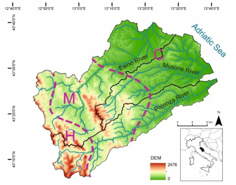
The study area (around 2600 km2), which includes the Musone (651 km2), Esino (1219 km2) and Potenza (775 km2) river basins, encompasses a wide territory of the Adriatic side of Central Italy, characterized by a typical mountain/high-hilly landscape in the central-western portion and few flat sectors located along the main alluvial plains and eastward, near the coast (Figure 1).

Figure 1. Location of the study area: H = high-hilly and mountain sector, M =

intermediate medium-low hilly sector, C = coastal sector.

More in detail, it can be generally divided into three longitudinal sectors, homogeneous in the range of altitudes and for their lithological (Figure 2a) and climatic (Figure 2b) characters [4−6]:

- a coastal sector (C), between 0m and 537m a.s.l. characterized by a clayey-sandy-conglomeratic bedrock and mean annual precipitation between 600 mm and 850 mm;

- an intermediate medium-low hilly sector (M), between 95m and 1475m a.s.l. with mainly arenaceous-conglomeratic and sandy-pelitic bedrock and mean annual precipitation between 850 mm and 1100 mm;

(4)

- an inner high-hilly and mountain sector (H), between 271 m and 1692 m a.s.l with the presence of mainly calcareous lithotypes and mean annual rainfalls between 1100 mm, and 1700 mm.

The trend of the average monthly temperatures and rainfalls, over the entire study area (calculated over the period 1950–2018) is shown in Figure 3.

a) b)

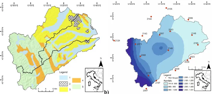
Figure 2. a) Schematic geological map of the Marche region. 1 = Main continental deposits

(Pliocene-Pleistocene-Holocene); 2 = Sands and conglomerates (Pliocene-Pleistocene); 3 = Clays and sands (Pliocene-Pleistocene; 4 = Arenaceous-marly-clayey turbidites (late Miocene); 5 = Limestones, marly limestones and marls (early Jurassic-Oligocene). b) Mean annual precipitation map of the Marche region. Larger symbols for the rain gauges indicate those employed in the hydrological model.

Figure 3. Histogram of the average monthly temperature and rainfalls. 0.00 5.00 10.00 15.00 20.00 25.00 0.00 10.00 20.00 30.00 40.00 50.00 60.00 70.00 80.00 90.00 100.00 Temperature [°C] Rainfall [mm] Rainfall Temperature

(5)

Such climatic features characterize what is currently defined as “Adriatic-sublitorial” regime [4]. The number of rainy days in this sector ranges between 60 and 75 while the daily mean intensity between 10 and 12 mm; the absolute monthly maximum is usually in November (secondary maximum in spring). Summer is rather dry, particularly near the coast, where periods without rainfall exceed 40 days. The mean annual temperatures on the other hand vary between 12.5 °C and 15.5 °C; the annual temperature excursion is around 18 °C, while the daily one goes from 7 °C along the coast to 10 °C in the intramountain basins. The Aridity Index—AI values varies from 19.9 to 38, defining an area which presents an average, slight summer aridity in the littoral portion and the low hills. The Modified Fournier erosivity Index—MFI ranges from 8.2. to 9.6 indicating a low erosion potential.

2.2. Rainfall data analysis

Hydrological modelling, as known, requires the definition of design storms or precipitation hyetographs. Design storms are then used as inputs to hydrological models, while the resulting flows and flow rates in a river basin are calculated using rainfall-runoff and flow routing procedures.

The present study calculates the design storm following the “Chicago Method”. This method establishes two different analytical equations for rainfall intensity over time, one valid before and another one valid after the peak rate, both derived from a Depth-Duration-Frequency (DDF) analytical expression, that preserves the same volumes of all rainfall intensities. Intensity-Duration-Frequency (DDF) curves, on the other hand, express in a synthetic way, for a given return time (T) (or its inverse, probability of exceedance) and a duration (t) of a rainfall event, the information on the maximum height of precipitation (h) and the maximum rainfall intensity (i). Generally, DDF curves can be described by the expression:

ℎ 𝑡, 𝑇 𝑎𝑡 (1)

in which a and n are parameters that have to be estimated through a probabilistic approach.

The cumulative probability function FX (x) represents the probability of not exceeding the value of the rainfall height h by that random variable. In this study, the cumulative distribution function used was the classical Generalized Extreme Value (GEV) Type-I distribution (or Gumbel distribution)

𝐹 𝑥 exp exp 𝑥 𝜉 𝛼⁄ (2)

where X is a random variable, x is a possible value of X, ξ is the location parameter calculated using 𝜇 𝜉 0.5772𝛼 and α is the scale parameter calculated using 𝜎 𝜋 𝛼 /6, where 𝜇 is the mean and 𝜎 the variance of the data set [7,8].

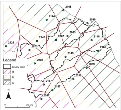
Rainfall data used in this study come from 18 weather stations, managed by the Marche Region Multi-risk Functional Center and considered representatives of the area analyzed (Figure 4). These weather station (whose characteristic parameters are given in Table 1) are distributed as follows:

- 10 in the coastal sector;

- 4 in the medium and low-hilly sector; - 4 in the high-hilly and mountainous sector.

(6)

Figure 4. Location of the study area with indication of the rain gauges used for the

statistical analysis. The map also shows the subdivision into areas of equal height of precipitation, processed through the Thiessen polygon method and the subdivision into climatic macro-areas: H = high-hilly and mountain sector, M = intermediate medium-low hilly sector, C = coastal sector.

Table 1. List of the rain gauges used in the study. Rain

Gauge

Gauge ID Zone x coord (m) y coord (m) Elevation (m a.s.l.) Missing Years (1950–2018) Missing Years (1998–2018) Macerata 2023 C 2394389 4795201 280 - - Tolentino 2038 C 2380482 4785380 244 - - Macerata 2039 C 2391814 4793706 232 - - Jesi 2063 C 2378238 4820428 96 4 - Maiolati Spontini 2067 C 2368749 4817949 110 1 - Ancona 2099 C 2395140 4829598 6 15 - Senigallia 2105 C 2376352 4841364 5 11 - Osimo 2148 C 2397421 4815699 265 30 - Recanati 2165 C 2402028 4806729 235 6 - Fabriano 2068 M 2350190 4800177 357 1 - Arcevia 2143 M 2353319 4818252 535 - - Corinaldo 2144 M 2362356 4834672 203 40 - Cingoli 2149 M 2375411 4803758 631 5 1 Camerino 2167 M 2362874 4777647 664 29 9 Serravalle di Chienti 2047 H 2353490 4771078 647 40 - Sassoferrato 2073 H 2346666 4811257 312 40 - Cantiano 2124 H 2328006 4815746 360 - - Pioraco 2157 H 2356279 4782617 441 2 -

(7)

To calculate the design storms, the maximum rainfall values recorded each year for durations of 1, 3, 6, 12 and 24 hours were collected for each rain gauge and, where available, for the period 1950–2018.

To verify the existence of a positive or negative trend of rainfall data and their statistical significance, the non-parametric Mann-Kendall and Sen’s slope estimator tests, very frequently used for the analysis of hydro-meteorological time series[9,10], were performed on both the “long” (1950–2018) and “short” (1998–2018) periods, to check also for possible changings.

The Mann-Kendall test S is generally calculated as:

𝑆 𝑠𝑔𝑛 𝑥 𝑥 (3)

where 𝑛 is the number of data points, 𝑥 and 𝑥 are the data values in time series 𝑖 and 𝑗 (𝑗 > 𝑖), respectively and 𝑠𝑔𝑛 𝑥 𝑥 is the sign function as:

𝑠𝑔𝑛 𝑥 𝑥

1, 𝑖𝑓 𝑥 𝑥 0

0, 𝑖𝑓 𝑥 𝑥 0

1, 𝑖𝑓 𝑥 𝑥 0

(4)

The variance is calculated as:

𝑉𝑎𝑟 𝑆 𝑛 𝑛 1 2𝑛 5 ∑ 𝑡 𝑡 1 2𝑡 5

18 (5)

where n is the number of data, m is the number of tied groups (i.e. sets of sample data having the same value) and ti is the number of ties of extent i. In cases where the sample size n > 10, the

standard normal test statistic Z is computed as follows:

𝑍 ⎩ ⎪ ⎨ ⎪ ⎧ 𝑆 1 𝑉𝑎𝑟 𝑆 , 𝑖𝑓 𝑆 0 0 𝑖𝑓 𝑆 0 𝑆 1 𝑉𝑎𝑟 𝑆 , 𝑖𝑓 𝑆 0 (6)

Positive values of 𝑍 indicate increasing trends while negative 𝑍 values show decreasing trends. Testing trends is usually done at a specific significance level. In this study, significance levels of 99% and 95% were used.

The Sen’s slope estimator test (Q) describes the slope of trend in the sample of N pairs of data:

𝑄 𝑥 𝑥

𝑗 𝑘 𝑓𝑜𝑟 𝑖 1, … . . 𝑁, (7)

where 𝑥 and 𝑥 are the data values at times j and 𝑘 (𝑗 > 𝑘), respectively.

The Q sign evidences data trend reflection, while its value indicates the steepness of the trend. To determine whether the slope is statistically different than zero, one should calculate the

(8)

confidence interval of Q at specific probability; same as for the Mann-Kendall test, significance levels of 99% and 95% have been chosen.

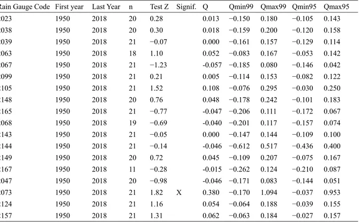
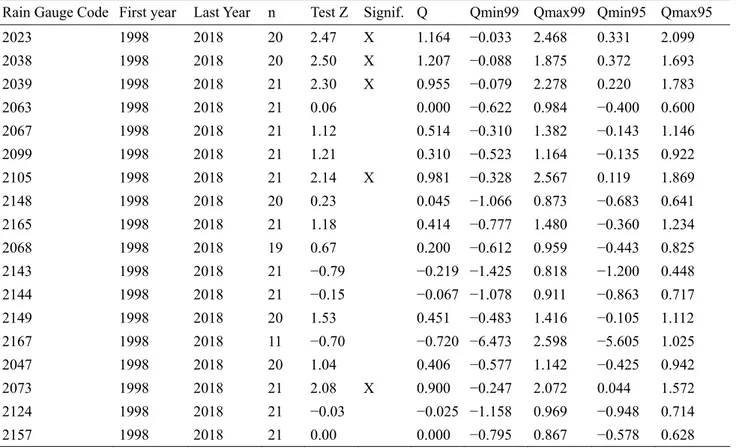
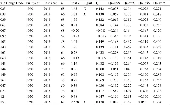
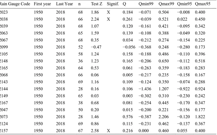
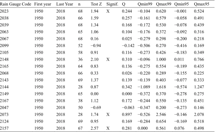
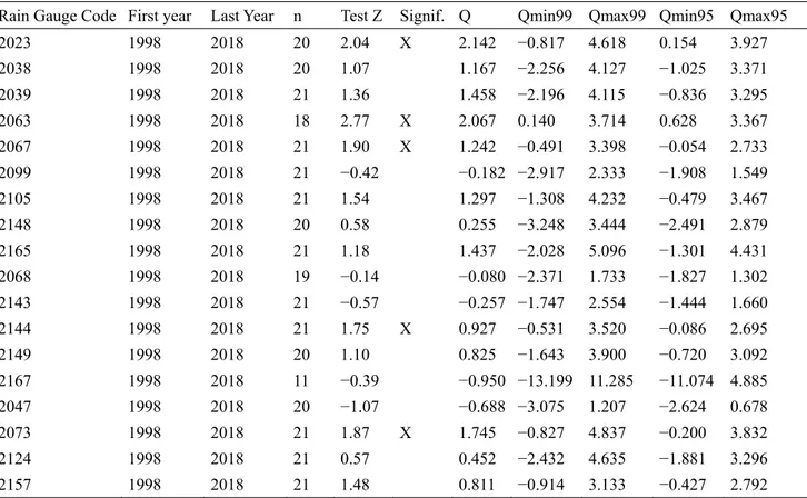
The results of the tests have shown in Table 2. From the analysis of results it is evident that only some weather stations register statistically significant trends; nevertheless, the latter always show a positive trend and the number of stations systematically increases (for all the durations analyzed) in the “short” period (1998–2018).

After this step, rainfall data were subsequently subjected to statistical analysis using the GEV Type I distribution to obtain the DDF curves. The spatialization of rainfall data over the whole study area functional to the use within the hydrologic model, has been finally implemented using the “Thiessen polygons” method [11]. Although other methods are also commonly used for the spatial distribution of rainfall data, the choice was here forced due to the software used for the hydrological modeling. As will be explained in more detail below, the association of specific design storm to each weather station within HEC-HMS, can only be achieved using the aforementioned tool; other methods only allow the insertion of a single maximum rainfall height, a procedure considered less suitable also for the successive calibration carried out with the observed river flow data.

Table 2A. Results of the statistical analysis carried out on different time series

(1950–2018; 1998–2018) and durations. (1 hour 1950–2018).

Rain Gauge Code First year Last Year n Test Z Signif. Q Qmin99 Qmax99 Qmin95 Qmax95

2023 1950 2018 20 0.28 0.013 −0.150 0.180 −0.105 0.143 2038 1950 2018 20 0.30 0.018 −0.159 0.200 −0.120 0.158 2039 1950 2018 21 −0.07 0.000 −0.161 0.157 −0.129 0.114 2063 1950 2018 18 1.10 0.052 −0.083 0.167 −0.053 0.142 2067 1950 2018 21 −1.23 -0.057 −0.185 0.080 −0.146 0.042 2099 1950 2018 21 0.21 0.005 −0.114 0.153 −0.082 0.122 2105 1950 2018 21 1.52 0.108 −0.076 0.295 −0.030 0.250 2148 1950 2018 20 0.76 0.048 −0.178 0.242 −0.101 0.183 2165 1950 2018 21 −0.77 -0.047 −0.206 0.111 −0.172 0.067 2068 1950 2018 19 −0.69 -0.040 −0.201 0.117 −0.157 0.074 2143 1950 2018 21 −0.05 0.000 −0.147 0.144 −0.109 0.100 2144 1950 2018 21 −0.14 -0.046 −0.612 0.517 −0.436 0.400 2149 1950 2018 20 0.72 0.045 −0.109 0.207 −0.075 0.167 2167 1950 2018 11 −0.28 -0.015 −0.262 0.124 −0.210 0.087 2047 1950 2018 20 −0.98 -0.046 −0.171 0.083 −0.144 0.051 2073 1950 2018 21 1.82 X 0.380 −0.170 1.094 −0.037 0.953 2124 1950 2018 21 1.16 0.054 −0.064 0.188 −0.039 0.155 2157 1950 2018 21 1.31 0.062 −0.063 0.184 −0.027 0.157

(9)

Table 2B. Results of the statistical analysis carried out on different time series

(1950–2018; 1998–2018) and durations. (1 hour 1998–2018).

Rain Gauge Code First year Last Year n Test Z Signif. Q Qmin99 Qmax99 Qmin95 Qmax95 2023 1998 2018 20 2.47 X 1.164 −0.033 2.468 0.331 2.099 2038 1998 2018 20 2.50 X 1.207 −0.088 1.875 0.372 1.693 2039 1998 2018 21 2.30 X 0.955 −0.079 2.278 0.220 1.783 2063 1998 2018 21 0.06 0.000 −0.622 0.984 −0.400 0.600 2067 1998 2018 21 1.12 0.514 −0.310 1.382 −0.143 1.146 2099 1998 2018 21 1.21 0.310 −0.523 1.164 −0.135 0.922 2105 1998 2018 21 2.14 X 0.981 −0.328 2.567 0.119 1.869 2148 1998 2018 20 0.23 0.045 −1.066 0.873 −0.683 0.641 2165 1998 2018 21 1.18 0.414 −0.777 1.480 −0.360 1.234 2068 1998 2018 19 0.67 0.200 −0.612 0.959 −0.443 0.825 2143 1998 2018 21 −0.79 −0.219 −1.425 0.818 −1.200 0.448 2144 1998 2018 21 −0.15 −0.067 −1.078 0.911 −0.863 0.717 2149 1998 2018 20 1.53 0.451 −0.483 1.416 −0.105 1.112 2167 1998 2018 11 −0.70 −0.720 −6.473 2.598 −5.605 1.025 2047 1998 2018 20 1.04 0.406 −0.577 1.142 −0.425 0.942 2073 1998 2018 21 2.08 X 0.900 −0.247 2.072 0.044 1.572 2124 1998 2018 21 −0.03 −0.025 −1.158 0.969 −0.948 0.714 2157 1998 2018 21 0.00 0.000 −0.795 0.867 −0.578 0.628

Table 2C. Results of the statistical analysis carried out on different time series

(1950–2018; 1998–2018) and durations. (3 hours 1950–2018).

2023 1950 2018 68 1.21 0.092 −0.104 0.284 −0.050 0.235 2038 1950 2018 66 0.20 0.017 −0.163 0.240 −0.114 0.173 2039 1950 2018 68 1.02 0.077 −0.100 0.261 −0.065 0.205 2063 1950 2018 65 0.97 0.073 −0.138 0.270 −0.086 0.207 2067 1950 2018 68 −0.65 −0.050 −0.222 0.147 −0.183 0.095 2099 1950 2018 52 −0.22 −0.020 −0.245 0.196 −0.197 0.127 2105 1950 2018 58 0.76 0.083 −0.181 0.400 −0.112 0.333 2148 1950 2018 36 1.01 0.059 −0.177 0.400 −0.086 0.309 2165 1950 2018 64 0.00 0.000 −0.224 0.200 −0.161 0.148 2068 1950 2018 66 −0.18 −0.015 −0.228 0.154 −0.164 0.120 2143 1950 2018 69 0.92 0.063 −0.107 0.245 −0.067 0.200 2144 1950 2018 28 −0.26 −0.086 −0.880 0.792 −0.648 0.585 2149 1950 2018 65 1.09 0.091 −0.139 0.312 −0.079 0.255 2167 1950 2018 38 −0.24 −0.021 −0.271 0.177 −0.213 0.117 2047 1950 2018 50 −0.24 −0.021 −0.227 0.194 −0.168 0.136 2073 1950 2018 28 0.43 0.110 −0.535 1.162 −0.387 0.805 2124 1950 2018 69 0.47 0.030 −0.146 0.200 −0.102 0.160 2157 1950 2018 67 2.00 X 0.109 −0.030 0.233 0.000 0.200

(10)

Table 2D. Results of the statistical analysis carried out on different time series

Rain Gauge Code First year Last Year n Test Z Signif. Q Qmin99 Qmax99 Qmin95 Qmax95 2023 1998 2018 20 2.82 X 1.51 0.116 2.951 0.465 2.539 2038 1998 2018 20 1.88 X 0.76 −0.400 2.325 −0.056 1.800 2039 1998 2018 21 2.63 X 1.23 0.041 2.600 0.304 2.230 2063 1998 2018 18 0.98 0.78 −1.171 3.145 −0.694 2.209 2067 1998 2018 21 1.99 X 0.73 −0.216 1.982 0.020 1.708 2099 1998 2018 21 0.06 0.03 −1.745 1.239 −1.020 0.855 2105 1998 2018 21 1.15 0.95 −1.058 2.933 −0.808 2.535 2148 1998 2018 20 0.81 0.267 −0.822 1.540 −0.468 1.200 2165 1998 2018 21 1.18 0.558 −1.161 1.982 −0.620 1.648 2068 1998 2018 19 0.42 0.250 −1.646 1.266 −0.883 1.087 2143 1998 2018 21 −1.24 −0.527 −1.688 0.611 −1.330 0.363 2144 1998 2018 21 0.60 0.269 −0.815 1.669 −0.587 1.325 2149 1998 2018 20 1.40 0.729 −0.638 1.813 −0.210 1.555 2167 1998 2018 11 −1.33 −1.533 −6.298 1.854 −5.464 1.134 2047 1998 2018 20 0.26 0.200 −1.010 1.162 −0.733 1.000 2073 1998 2018 21 1.69 X 0.530 −0.400 2.583 −0.103 1.936 2124 1998 2018 21 1.03 0.329 −0.795 1.433 −0.422 1.000 2157 1998 2018 21 −0.03 −0.029 −0.937 0.918 −0.731 0.682

Table 2E. Results of the statistical analysis carried out on different time series

Rain Gauge Code First year Last Year n Test Z Signif. Q Qmin99 Qmax99 Qmin95 Qmax95 2023 1950 2018 68 1.65 X 0.143 −0.078 0.356 −0.026 0.291 2038 1950 2018 66 1.81 X 0.138 −0.057 0.370 −0.014 0.318 2039 1950 2018 68 1.59 0.122 −0.067 0.319 −0.025 0.260 2063 1950 2018 65 0.91 0.084 −0.144 0.336 −0.082 0.255 2067 1950 2018 68 −0.20 −0.013 −0.214 0.164 −0.167 0.120 2099 1950 2018 52 −0.73 −0.083 −0.385 0.205 −0.314 0.136 2105 1950 2018 58 1.04 0.149 −0.168 0.467 −0.110 0.400 2148 1950 2018 36 1.28 0.139 −0.181 0.467 −0.083 0.369 2165 1950 2018 64 0.28 0.033 −0.208 0.266 −0.147 0.200 2068 1950 2018 66 −0.13 −0.005 −0.190 0.161 −0.143 0.117 2143 1950 2018 69 1.16 0.082 −0.107 0.294 −0.057 0.243 2144 1950 2018 28 0.00 0.000 −1.051 1.040 −0.763 0.734 2149 1950 2018 65 0.99 0.108 −0.155 0.356 −0.100 0.289 2167 1950 2018 38 0.72 0.069 −0.230 0.350 −0.153 0.253 2047 1950 2018 50 0.36 0.030 −0.192 0.227 −0.143 0.176 2073 1950 2018 28 0.38 0.117 −0.582 1.894 −0.405 1.395 2124 1950 2018 69 0.68 0.047 −0.150 0.263 −0.100 0.200 2157 1950 2018 67 2.538 X 0.178 −0.002 0.382 0.056 0.334

(11)

Table 2F. Results of the statistical analysis carried out on different time series

(1950–2018; 1998–2018) and durations. (6 hours 1998–2018).

Rain Gauge Code First year Last Year n Test Z Signif. Q Qmin99 Qmax99 Qmin95 Qmax95 2023 1998 2018 20 1.95 X 1.050 −0.290 2.858 −0.004 2.465 2038 1998 2018 20 1.46 0.939 −0.637 2.172 −0.338 1.981 2039 1998 2018 21 1.45 0.719 −0.624 2.600 −0.192 2.200 2063 1998 2018 18 1.29 0.860 −0.979 3.406 −0.556 2.592 2067 1998 2018 21 2.78 X 0.898 0.100 2.127 0.277 1.849 2099 1998 2018 21 −0.27 −0.194 −2.837 1.623 −2.311 1.072 2105 1998 2018 21 1.18 1.077 −1.339 3.365 −0.623 2.778 2148 1998 2018 20 0.58 0.253 −1.323 1.800 −0.893 1.412 2165 1998 2018 21 0.57 0.440 −1.288 2.113 −0.720 1.737 2068 1998 2018 19 −0.07 −0.010 −1.676 0.832 −0.722 0.600 2143 1998 2018 21 −0.94 −0.447 −1.703 1.051 −1.306 0.687 2144 1998 2018 21 0.94 0.510 −0.815 1.846 −0.533 1.600 2149 1998 2018 20 1.8828 X 0.914 −0.333 2.485 −0.057 1.933 2167 1998 2018 11 −0.93 −1.489 −5.885 4.135 −4.599 1.393 2047 1998 2018 20 0.13 0.075 −1.167 1.306 −0.736 0.960 2073 1998 2018 21 1.27 0.640 −0.547 3.896 −0.255 3.180 2124 1998 2018 21 0.97 0.544 −1.150 1.580 −0.605 1.333 2157 1998 2018 21 0.82 0.289 −1.098 2.196 −0.741 1.781

Table 2G. Results of the statistical analysis carried out on different time series

Rain Gauge Code First year Last Year n Test Z Signif. Q Qmin99 Qmax99 Qmin95 Qmax95 2023 1950 2018 68 1.86 X 0.184 −0.071 0.504 −0.008 0.400 2038 1950 2018 66 2.24 X 0.261 −0.039 0.521 0.022 0.450 2039 1950 2018 68 1.07 0.120 −0.161 0.421 −0.095 0.342 2063 1950 2018 65 1.59 0.139 −0.108 0.388 −0.049 0.320 2067 1950 2018 68 0.35 0.034 −0.212 0.274 −0.154 0.225 2099 1950 2018 52 −0.47 −0.056 −0.368 0.248 −0.280 0.173 2105 1950 2018 58 1.24 0.158 −0.188 0.486 −0.110 0.396 2148 1950 2018 36 1.23 0.165 −0.206 0.650 −0.112 0.518 2165 1950 2018 64 0.53 0.061 −0.263 0.359 −0.183 0.283 2068 1950 2018 66 0.06 0.005 −0.217 0.235 −0.158 0.167 2143 1950 2018 69 1.16 0.109 −0.124 0.350 −0.074 0.288 2144 1950 2018 28 0.16 0.106 −1.436 1.207 −0.922 0.924 2149 1950 2018 65 0.03 0.003 −0.302 0.310 −0.230 0.242 2167 1950 2018 38 0.68 0.081 −0.254 0.445 −0.170 0.347 2047 1950 2018 50 0.20 0.015 −0.200 0.221 −0.156 0.177 2073 1950 2018 28 1.46 0.576 −0.387 2.206 −0.120 1.822 2124 1950 2018 69 0.86 0.115 −0.231 0.462 −0.137 0.367 2157 1950 2018 67 2.58 X 0.216 0.000 0.460 0.055 0.400

(12)

Table 2H. Results of the statistical analysis carried out on different time series

2023 1998 2018 20 1.07 1.034 −1.208 3.624 −0.642 3.147 2038 1998 2018 20 1.27 0.790 −1.133 2.820 −0.513 2.655 2039 1998 2018 21 0.51 0.588 −1.538 3.220 −1.106 2.478 2063 1998 2018 18 2.35 X 1.600 −0.156 3.020 0.467 2.605 2067 1998 2018 21 2.39 X 1.215 −0.213 2.400 0.286 2.057 2099 1998 2018 21 −0.48 −0.335 −2.736 1.562 −1.838 1.056 2105 1998 2018 21 1.36 1.247 −1.447 3.343 −0.751 3.065 2148 1998 2018 20 0.19 0.090 −2.298 2.761 −1.716 2.253 2165 1998 2018 21 0.73 0.445 −1.805 2.585 −1.133 2.035 2068 1998 2018 19 0.11 0.038 −2.400 1.741 −1.679 1.290 2143 1998 2018 21 −0.73 −0.335 −1.764 1.645 −1.452 1.018 2144 1998 2018 21 1.39 0.547 −0.563 2.863 −0.232 2.129 2149 1998 2018 20 1.36 0.883 −0.757 3.059 −0.393 2.577 2167 1998 2018 11 −0.31 −1.267 −10.606 6.516 −7.341 5.199 2047 1998 2018 20 −0.13 −0.049 −1.745 1.636 −1.338 1.007 2073 1998 2018 21 1.78 X 1.183 −0.400 4.731 −0.080 3.713 2124 1998 2018 21 0.85 0.646 −1.574 3.049 −0.928 2.634 2157 1998 2018 21 0.82 0.452 −1.000 2.646 −0.700 2.218

Table 2I. Results of the statistical analysis carried out on different time series

Rain Gauge Code First year Last Year n Test Z Signif. Q Qmin99 Qmax99 Qmin95 Qmax95 2023 1950 2018 68 1.94 X 0.244 −0.104 0.620 −0.001 0.524 2038 1950 2018 66 1.59 0.257 −0.161 0.579 −0.058 0.491 2039 1950 2018 68 1.34 0.168 −0.172 0.530 −0.078 0.439 2063 1950 2018 65 1.06 0.104 −0.176 0.372 −0.092 0.316 2067 1950 2018 68 0.16 0.025 −0.279 0.298 −0.200 0.218 2099 1950 2018 52 −0.94 −0.142 −0.506 0.270 −0.416 0.169 2105 1950 2018 58 0.91 0.116 −0.273 0.426 −0.183 0.349 2148 1950 2018 36 2.10 X 0.310 −0.096 1.000 0.011 0.766 2165 1950 2018 64 0.83 0.136 −0.275 0.554 −0.189 0.435 2068 1950 2018 66 0.33 0.026 −0.220 0.289 −0.155 0.225 2143 1950 2018 69 1.37 0.139 −0.139 0.403 −0.077 0.333 2144 1950 2018 28 0.87 0.342 −1.089 1.618 −0.574 1.247 2149 1950 2018 65 0.00 0.000 −0.372 0.370 −0.278 0.275 2167 1950 2018 38 1.12 0.172 −0.244 0.550 −0.135 0.451 2047 1950 2018 50 −0.69 −0.063 −0.347 0.200 −0.273 0.146 2073 1950 2018 28 1.74 X 0.897 −0.526 2.546 −0.146 2.078 2124 1950 2018 69 0.95 0.169 −0.284 0.654 −0.169 0.518 2157 1950 2018 67 2.57 X 0.281 0.000 0.561 0.076 0.498

(13)

Table 2J. Results of the statistical analysis carried out on different time series

Rain Gauge Code First year Last Year n Test Z Signif. Q Qmin99 Qmax99 Qmin95 Qmax95 2023 1998 2018 20 2.04 X 2.142 −0.817 4.618 0.154 3.927 2038 1998 2018 20 1.07 1.167 −2.256 4.127 −1.025 3.371 2039 1998 2018 21 1.36 1.458 −2.196 4.115 −0.836 3.295 2063 1998 2018 18 2.77 X 2.067 0.140 3.714 0.628 3.367 2067 1998 2018 21 1.90 X 1.242 −0.491 3.398 −0.054 2.733 2099 1998 2018 21 −0.42 −0.182 −2.917 2.333 −1.908 1.549 2105 1998 2018 21 1.54 1.297 −1.308 4.232 −0.479 3.467 2148 1998 2018 20 0.58 0.255 −3.248 3.444 −2.491 2.879 2165 1998 2018 21 1.18 1.437 −2.028 5.096 −1.301 4.431 2068 1998 2018 19 −0.14 −0.080 −2.371 1.733 −1.827 1.302 2143 1998 2018 21 −0.57 −0.257 −1.747 2.554 −1.444 1.660 2144 1998 2018 21 1.75 X 0.927 −0.531 3.520 −0.086 2.695 2149 1998 2018 20 1.10 0.825 −1.643 3.900 −0.720 3.092 2167 1998 2018 11 −0.39 −0.950 −13.199 11.285 −11.074 4.885 2047 1998 2018 20 −1.07 −0.688 −3.075 1.207 −2.624 0.678 2073 1998 2018 21 1.87 X 1.745 −0.827 4.837 −0.200 3.832 2124 1998 2018 21 0.57 0.452 −2.432 4.635 −1.881 3.296 2157 1998 2018 21 1.48 0.811 −0.914 3.133 −0.427 2.792 2.3. Land use

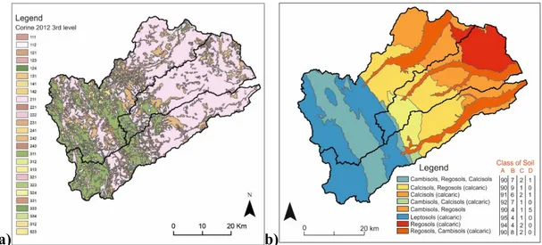
Concerning the land use, vector data from the IIIrd level of the CORINE Land Cover 2012 inventory (CLC-2012)[12] have been collected (Figure 5a); the analysis of data, evidences that around 68% is characterized by agricultural areas, 27% by Forest and Seminatural areas and only 5% by Artificial surfaces. The characteristics of the soils, on the other hand, have been extrapolated generalizing and integrating data from the Soil Map of the Marche Region at 1: 250,000 scale. The different types of soil have been merged according to the World Reference Base for Soil Resources—WRB [13]. Four main groups of the WRB characterize the study area: Cambisols, Leptosols, Regosols, Calcisols.

Cambisols, very common in temperate and boreal regions, are brownish soils with weak horizon differentiation and characterized by the presence of a cambic horizon (Bw), below the organic-mineral one. These soils are predominant in the sedimentary basin placed within the calcareous ridges of the Apennine chain. Leptosols are very shallow soils with minimal development, formed typically on hard rock or highly calcareous materials; in the study area they are present along the Apennine ridges and are mainly developed over colluvial and slope quaternary deposits. Regosols, mostly developed along the alluvial plains, are usually not shallow enough to be Leptosols and consist of very weakly developed mineral soils in unconsolidated materials with only an ochric surface horizon. Calcisols, finally, are soils with a significant secondary accumulation of calcium carbonate and are common on the low-hilly areas of the region where a mainly pelitic and sandy-pelitic bedrock outcrops.

(14)

a) b)

Figure 5. a) Corine Land use map (3rd Level): numbers are reported according to the

official legend; b) Soil Classes Map.

All these groups are characterized by dominant calcareous horizons, in line with the geological features of the territory and are usually well-drained soils with fine to medium texture; given their high spatial variability, a further generalization was carried out in order to obtain more homogeneous areas, in agreement with the geomorphological characteristics of the territory (Figure 5b). According to the NRCS (Natural Resource Conservation Service) hydrologic method [14], for each type of soil have been assigned values as a percentage of the Hydrologic Soil Groups classified as follows on the base on their infiltration rate:

- Group A: soils with low runoff potential and high infiltration rate even when thoroughly wetted. They consist mainly of deep, well drained sand or gravel and have a high rate of water transmission (greater than 7.6 mm/hr).

- Group B: soils with moderate infiltration rate when thoroughly wetted and consist of moderately deep to deep, moderately well to well drained soils with moderately fine to moderately coarse textures. They have a moderate rate of water transmission (3.8–7.6 mm/hr). - Group C: soils with low infiltration rate when thoroughly wetted and consist chiefly of soils with a layer that inhibits downward movement of water and soils with moderately fine to fine texture. They have a low rate of water transmission (1.3–3.8 mm/hr).

- Group D: soils with high runoff potential. They have very low infiltration rate when thoroughly wetted, they may contain a permanent water table and consist of clay soils with a high swelling potential, shallow soils over nearly impervious material and may contain a claypan or clay layer at or near the surface. These soils have a very low rate of water transmission (0–1.3 mm/hr).

2.4. Hydrological modeling

The hydrological model for the study area was realized through two distinct phases. In a former phase, data concerning the morphometry and the hydro-geomorphological characteristics of the river basins (land use, soil type etc) were preprocessed using the tools for ArcGIS “HEC-GeoHMS” version 10.2, developed by the U.S. Army Corps of Engineers [15]. This software allows to process

(15)

spatial data to obtain dimensional, morphological and hydrological characteristics of the river basins. These data were subsequently used to perform hydrological simulations through HEC-HMS software v. 4.3, also developed by the U.S. Army Corps of Engineers [16].

The morphological characterization of the river basins through HEC-GeoHMS was carried out using a 1m high-resolution DTM (obtained processing LiDAR images provided by the Italian Ministry of Environment): this allows to disaggregate the three watersheds (Musone, Esino and Potenza) into a series of interconnected sub-basins (50 in total) and to divide the stream networks in reaches and junctions (Figure 6a). Physical characteristics such as the river length and slope, subbasin slope, subbasin centroid location and elevation, longest flow have been also extracted. The evaluation of the hydrological parameters (necessary for the subsequent calculation of infiltration and runoff coefficients in HEC-HMS) was then performed by applying the “Curve Number” method, developed by the Soil Conservation Service of the United States. The method provides the computation of the parameter Curve Number (CN), a dimensionless parameter that ranges between 0 and 100 and expresses the capacity of the soil to produce direct runoff: the higher the value the greater the runoff produced with the same rainfall. A grid file of the Curve Number was obtained by geoprocessing operation in ArcGIS, combining the previously created shapefiles of the land use and of the soil type (Figure 6b).

a) b)

Figure 6. a) HEC-HMS schematization and watershed delineation; different colors

indicate different river basins. b) The Curve Number (CN) map of the study area.

The variability in the CN depends on several factors as rainfall intensity and duration, soil moisture conditions, vegetation cover, temperature; these factors are collectively called Antecedent Runoff Conditions (ARCs). ARCs are divided into three classes: II for average conditions, I for dry conditions, and III for wet conditions [17]. Taking into account the purpose of the work, i.e. the runoff computation in critical conditions, the ARCs III were chosen and the initial grid file (corresponding to the ARCs II) was modified according to the following formula:

𝐶𝑁 𝐴𝑅𝐶𝑠 𝐼𝐼𝐼 𝐶𝑁 𝐴𝑅𝐶𝑠 𝐼𝐼

(16)

The CN values thus obtained can be considered reliable, as they are in line with those obtained in previous studies through calibration procedures with real events (Materazzi, 2015).

3. Results and discussion

The rainfalls series collected for each of the 18 rain gauges, as described in chapter 2b, have been processed for the construction of the DDF curves for different event durations, return times and length of the time series (Figure 7a). More specifically, for each rain gauge, the analysis was performed on:

- two historical series (1951–2018; 1998–2018) - five durations (1, 3, 6, 12, 24 hours)

- two return times: 100 yrs (corresponding to an Annual Exceedance Probability—AEP of 1%) and 200 yrs (corresponding to an Annual Exceedance Probability—AEP of 0.5%). The results of this analysis are globally shown in Table 3.

a)

b)

Figure 7. a) DDF curves and b) Chicago-type hyetograph relative to the rain gauge of

Senigallia. 0.00 50.00 100.00 150.00 200.00 250.00 0 5 10 15 20 25 Tr=100 Tr=200 0.0 5.0 10.0 15.0 20.0 25.0 30.0 35.0 40.0 45.0 0 100 200 300 400

(17)

For each rain gauge (and consequently for each return time and for both series analyzed) the Chicago-type hyetographs was computed; these hyetographs (Figure 7b) were later used as input within each of the 12 HEC-HMS hydrological models (3 river basins × 2 return times × 2 rainfalls series). The regionalization of the rainfall data, as mentioned in paragraph 2b, was carried out using the Thiessen polygon method.

Table 3. a and n coefficient calculated for different return times and different lengths of

the rainfalls series.

1951–2018

Rain Gauge ID

1998–2018

100 years 200 years 100 years 200 years

a n a n a n a N 54.615 0.2988 60.07 0.2982 2039 57.987 0.3155 64.098 0.3132 62.173 0.2575 68.404 0.2552 2038 74.051 0.2687 82.329 0.2663 50.442 0.304 54.828 0.3038 2047 53.943 0.3058 58.695 0.3068 65.038 0.2261 71.92 0.2239 2068 53.572 0.2671 58.574 0.267 77.785 0.2575 87.368 0.2538 2148 90.076 0.2565 101.44 0.252 64.809 0.2812 71.392 0.2802 2149 56.107 0.3069 61.164 0.3071 47.735 0.353 51.951 0.3546 2157 48.678 0.4067 52.839 0.41 63.945 0.2852 70.601 0.2839 2165 74.051 0.2687 82.329 0.2663 62.538 0.2703 69.53 0.2664 2167 66.76 0.2891 73.955 0.2851 84.021 0.2284 93.694 0.225 2105 89.232 0.1889 99.406 0.1846 54.593 0.3454 59.865 0.3457 2144 50.016 0.3578 54.755 0.359 59.104 0.325 65.107 0.3252 2099 52.491 0.3409 57.357 0.3424 58.046 0.2672 64.265 0.2638 2063 71.702 0.1516 79.596 0.1426 88.903 0.2738 99.831 0.2717 2073 98.563 0.2704 110.89 0.2683 54.615 0.2988 60.07 0.2982 2023 57.987 0.3155 64.098 0.3132 56.03 0.2635 61.488 0.261 2143 53.358 0.3164 58.338 0.3156 52.226 0.4392 57.328 0.4432 2067 51.985 0.4723 56.788 0.4787 57.053 0.3628 62.491 0.3617 2124 61.979 0.3396 67.877 0.3369

Once the design storm was developed, the basin model was defined in HEC-HMS. Some data relating to the sub-basins (including the NC), previously calculated in HEC-GeoHMS, were automatically imported into the model. The time of corrective action was instead calculated using the Kirpich Method, developed for small drainage basins in Tennessee and Pennsylvania, with basin areas from 1 to 112 acres

𝑇𝑐 0.0078𝐿 . 𝐿

𝐻

.

(9)

where Tc is the time of concentration in minutes, L is the maximum hydraulic flow length in feet, and H is the difference in elevation in feet between the outlet of the watershed and the hydraulically most remote point in the watershed. Basing on the values obtained, a duration of 6 hours for the design storm of each rain gauge, in line with the time of concentration of all the sub-basins, was chosen. “Net rain” and “rainfall-runoff transformation process” were finally evaluated by applying

(18)

the Soil Conservation Service methods, as the SCS Curve Number Loss and the SCS Unit Hydrograph Transform respectively.

Concerning the river reaches the choice of the routing procedure fell on the SCS Lag method, which is best suited for short stream segments with a predicable travel time that doesn’t vary with flow depth. Once the data has been entered, the simulation has been started for each of the models provided. The results are shown in Table 4.

Table 4. Flow rate values calculated for different return times and different lengths of the

rainfalls series: the fourth column shows the percentage variation of the second series compared to the first.

Q [m3_{/s] 100 yrs 1951–2018} _{Q [m}3_{/s] 100 yrs 1998–2018} _{Variation [%]}

Potenza-Subbasin W1070 44.7 51.9 16.11 W1080 28.7 25.9 −9.76 W1130 30.6 33.8 10.46 W1180 63.1 61.5 −2.54 W1190 77.5 86.8 12.00 W1280 88.6 105.1 18.62 W1410 18 24.9 38.33 W1500 24.9 32.4 30.12 W1520 48.2 59 22.41 W1610 42.4 56 32.08 W1740 21.5 28.1 30.70 W940 42.1 48.8 15.91 W950 52.6 62.8 19.39 W970 72.9 88.6 21.54 W1070 54.3 62.7 15.47 W1080 34.9 31.4 −10.03 W1130 37.1 40.8 9.97 W1180 75.2 72.9 −3.06 W1190 94 104.7 11.38 W1280 104.4 123.1 17.91 W1410 23.2 31.5 35.78 W1500 32.5 41.3 27.08 W1520 56.5 68.6 21.42 W1610 55.3 71.5 29.29 W1740 27.4 35.4 29.20 W940 51 58.9 15.49 W950 60.9 72.9 19.70 W970 86.1 104.6 21.49

(19)

Q [m3_{/s] 100 yrs 1951–2018} _{Q [m}3_{/s] 100 yrs 1998–2018} _{Variation [%]} Esino-Subbasin W1060 67.8 80.7 19.027 W1160 171.3 146 −14.769 W1170 85.5 73.3 −14.269 W1260 106.2 118.3 11.394 W1280 12.6 12.6 0.000 W1290 79.1 77.1 −2.528 W720 18 17.9 −0.556 W730 58.4 48.5 −16.952 W780 29.1 30.5 4.811 W820 26.4 25.7 −2.652 W840 120 104.6 −12.833 W910 100.9 97 −3.865 W930 135.4 160.5 18.538 W940 161.4 177.9 10.223 W950 54.5 44.4 −18.532 W1060 79.3 102.1 28.75 W1160 195.7 164.9 −15.74 W1170 99.9 85 −14.91 W1260 123.6 137 10.84 W1280 16.7 16.4 −1.80 W1290 92.7 90.2 −2.70 W720 22.7 22.2 −2.20 W730 70.7 58.6 −17.11 W780 37.6 39 3.72 W820 34.9 33.6 −3.72 W840 140.5 122 −13.17 W910 116.2 111.3 −4.22 W930 168.4 198.7 17.99 W940 188.9 208.1 10.16 W950 66.3 53.5 −19.31

(20)

Q [m3_{/s] 100 yrs 1951–2018} _{Q [m}3_{/s] 100 yrs 1998–2018} _{Variation [%]} Musone-Subbasin W1050 68.6 92 34.11 W1080 72.4 66.3 −8.43 W1100 54.2 44.1 −18.63 W1240 71.6 56.7 −20.81 W1300 64.9 50.1 −22.80 W680 29.7 25.3 −14.81 W690 25.1 22.7 −9.56 W700 26.4 33.5 26.89 W720 36.2 42.2 16.57 W730 17.8 23 29.21 W750 37.5 50.1 33.60 W760 32.0 44 37.50 W800 37.5 53 41.33 W810 26.1 34.1 30.65 W820 34.5 46.6 35.07 W850 32.5 43.2 32.92 W860 63.9 75.6 18.31 W940 52.3 69.5 32.89 W950 55.9 68.2 22.00 W960 56.9 72.9 28.12 W970 66.4 85.3 28.46 W1050 84.2 112.0 33.02 W1080 88.1 80.1 −9.08 W1100 67 54.0 −19.40 W1240 88.7 69.7 −21.42 W1300 82.9 63.9 −22.92 W680 31.4 33.2 5.73 W690 26.4 28.4 7.58 W700 32.1 42.2 31.46 W720 42.2 52.1 23.46 W730 21.8 28.8 32.11 W750 45.8 60.7 32.53 W760 39.9 54.2 35.84 W800 47.6 66.8 40.34 W810 31.4 40.8 29.94 W820 42.4 56.7 33.73 W850 39.8 52.4 31.66 W860 78.3 92.1 17.62 W940 63.6 84.2 32.39 W950 68.4 82.8 21.05 W960 68.1 87.0 27.75 W970 80.6 103.3 28.16

(21)

For each basin analyzed, the table shows the list of sub-basins, the flow rate calculated for different return times (100 yrs or 200 yrs) and for the two historical series analyzed (1951–2018 or 1998–2018). The rightmost column, with different colors, indicates the percentage variations (positive or negative) of the flow rate calculated from the most recent rainfall series compared to the longer one. In particular, red color evidences flow rate increase, green color flow rate decrease, yellow color positive or negative deviations not exceeding 10%; this latter value takes into account the uncertainty and the number of rain gauges (not high) used for the statistical analysis.

The analysis of results, clearly shows that most of the Potenza and Musone sub-basins, if modeled using the rainfall series 1998–2018, increases more than 30% the flow rate for both 100 yrs and 200 yrs return times. The Musone river, on the other hand, has a more uncertain behavior. On the other hand, observing the same results in Figure 8a,b (where the areas of the Thiessen polygons are also reported) it is evident that most of the "uncertain" percentage variations (within a range of ±10%) are only associated with 3–4 rain gauges, while those negative essentially to only one. These apparent rainfalls anomalies, once the quality of data coming from these sensors has been verified, will require future climatological insights.

Figure 8. Modeling results: percentage variation between flow rate calculated using

1998–2018 series and 1951–2018 series for a) Tr = 100 yrs and b) Tr = 200 yrs. Red color indicates positive variations (> 10%); green color, negative variations (< −10%); yellow color, no significant variations (between −10% and +10%).

4. Conclusions

The present work, comparing the results of hydrological models derived from statistical analyses of different historical rainfalls series showed that:

- Mann-Kendall and Sen’s Slope estimator tests evidenced a positive, although weak and not evenly distributed, positive trend of rainfall starting from 1950; this trend is slightly more evident for the period 1998–2018;

(22)

- the DDF curves of 18 pluviometers uniformly distributed in the study area, calculated using a recent rainfalls series (1998–2018), show heights of precipitation significantly higher than those derived from a longer rainfall series (1951–2018) for the return times considered (100 yrs and 200 yrs);

- Chicago-type design storms, calculated from the recent rainfalls series, generate higher flood rates when entered as input data in a hydrological model;

- the hydrological model developed for the study area shows how the flow rate generated by the use of the 1998–2018 pluviometric series is in many cases more than 30% higher than the other;

- values apparently in contrast with those cited are to be associated with the response of few, single sensors whose reliability have to be verified or adequately justified from a climatological point of view;

- the results obtained by the present study, although preliminary and limited to a small sector of central Italy, show that the ongoing ascertained climate change is associated with a change in the rainfall regime, turning towards an increase in rainfall intensity and frequency of extreme events;

- the use of recent but short rainfall series, although less significant from a statistical point of view, can therefore be more reliable if included in a numerical modeling for the definition of future risk scenarios.

Acknowledgments

The authors want to thank Consorzio di Bonifica delle Marche for kindly providing all the data. ORCID:

Margherita Bufalini: https://orcid.org/0000-0003-3278-7058 Marco Materazzi: https://orcid.org/0000-0002-9480-5680

Conflict of interest

No potential conflict of interest was reported by the authors.

References

1. Masson-Delmotte V, Zhai P, Pörtner H, et al. (2018) An IPCC Special Report on the impacts of global warming of 1.5 °C above pre-industrial levels and related global greenhouse gas emission pathways, in the context of strengthening the global response to the threat of climate change, sustainable development, 24.

2. Huong HTL, Pathirana A (2013) Urbanization and climate change impacts on future urban flooding in Can Tho city, Vietnam. Hydrol Earth Syst Sci 17: 379–394.

3. Sperotto A, Torresan S, Gallina V, et al. (2016) A multi-disciplinary approach to evaluate pluvial floods risk under changing climate: The case study of the municipality of Venice (Italy). Sci Total Environ 562: 1031–1043.

4. Amici M, Spina R (2002) Campo medio della precipitazione annuale e stagionale sulle Marche per il periodo 1950–2000, 103.

(23)

5. Gentilucci M, Bisci C, Burt P, et al. (2018) Interpolation of Rainfall through Polynomial Regression in the Marche Region (Central Italy), Springer International Publishing.

6. Pierantoni P, Deiana G, Galdenzi S (2013) Stratigraphic and structural features of the sibillini mountains(Umbria- Marche Apennines, Italy). Ital J Geosci 132: 497–520.

7. Gumbel EJ (1941) Probability‐interpretation of the observed return‐periods of floods. Eos, Trans Am Geophys Union 22: 836–850.

8. Gumbel EJ (1954) Statistical theory of extreme values and some practical applications. Appl Math Ser 33: 341–342.

9. Tabari H, Talaee PH (2011) Analysis of trends in temperature data in arid and semi-arid regions of Iran. Glob Planet Change 79: 1–10.

10. Gocic M, Trajkovic S (2013) Analysis of changes in meteorological variables using Mann-Kendall and Sen’s slope estimator statistical tests in Serbia. Glob Planet Change 100: 172–182.

11. Thiessen AH (1911) Precipitation for large areas. Mon Weather Rev 39: 1082–1084. 12. NBGC (2006) Valter Sambucini, Ines Marinosci, CORINE LAND COVER 2006 (ISPRA).

13. Food and Agriculture Organization of the United Nations (2015) International soil classification system for naming soils and creating legends for soil maps.

14. USDA-NRCS (2009) National Engineering Handbook Chapter 7: Hydrologic Soil Groups. Part 630 Hydrol Natl Eng Handb, 5.

15. Fleming MJ, Doan JH (2013) HEC-GeoHMS geospatial hydrologic modeling extension.

16. Scharffenberg B, Bartles M, Brauer T, et al. (2018) Hydrologic Modeling System User’s Manual. 17. USDA-NRCS (2009) Hydrology National Engineering Handbook Chapter 10 Estimation of

Direct Runoff from Storm Rainfall. Part 630 Hydrol Natl Eng Handb.