An experiment in autonomous navigation for a security robot

(1)

POLITECNICO DI MILANO MSc in Computer Science and Engineering Scuola di Ingegneria Industriale e dell’Informazione Dipartimento di Elettronica, Informazione e Bioingegneria

AN EXPERIMENT IN AUTONOMOUS

NAVIGATION FOR A SECURITY

ROBOT

AI & R Lab

Laboratorio di Intelligenza Artificiale e Robotica del Politecnico di Milano

Supervisor: Prof. Matteo Matteucci Co-supervisor: Ing. Gianluca BARDARO

Master Graduation Thesis by: Fabio Santi VENUTO, Student ID 837644

(2)

(3)

(4)

(5)

Abstract

One of the most useful purpose in self driving autonomous robots is to substitute for human activity in dangerous and heavy jobs. The Ra.Ro platform, developed by NuZoo, is designed to work as a security robot, able to patrol, detect and eventually send alarm to a centralized station. This platform is often required to be adapted to different purposes, but most of them require an autonomous navigation. The aim of this thesis is to propose a mapping and localization system to avoid the well-known drifting problem. In particular we are dealing with the indoor environment, which is challenging because is not available any fixed point reliable sensor such as GPS. The odometry system provided by the wheel encoders is not precise enough and very sensitive to errors, thus it is important to fuse the information retrieved by multiple sensors such as IMU, LIDAR and a camera used to recognize specific markers.

The final results, tested in the real world, are quite satisfying at the end, but can be further improved.

(6)

(7)

Sommario

Uno dei principali scopi di robot a guida autonoma è quello di sostituire l’uomo nelle attività più pericolose a nei lavori più pesanti. La piattaforma Ra.Ro., sviluppata da NuZoo, è progettata per lavorare come robot di si-curezza, capace di pattugliare, individuare e infine lanciare un allarme ad una stazione centralizzata. Spesso è stato richiesto che questa piattaforma venga adattata per diversi scopi, ma la maggior parte di essi richiedono una navigazione autonoma. L’obbiettivo di questa tesi è di proporre un sistema di mappatura e localizzazione che ovvi al noto problema del drifting. In par-ticolare ci occupiamo di un ambiente interno, il quale è difficoltoso a causa della mancanza di un sensore, come il GPS, che ci dia informazioni affid-abili su dei punti fissi. Il sistema di odometria fornito dagli encoder delle ruote non è abbastanza preciso e molto sensibile agli errori, per questo è molto importante fondere le infomazioni ricevute da molteplici sensori quali una IMU, un LIDAR e una videocamera utilizzata per riconoscere marker specifici.

I risultati, testati in un ambiente reale, sono stati soddisfacenti alla fine, ma possono essere ancora migliorati.

(8)

(9)

Ringraziamenti

Ringrazio ...

(10)

(11)

Introduction

“Narrator: Deep in the Caribbean, Scabb Island.

Guybrush: ...So I bust into the church and say, “Now you’re in for it, you bilious bag of barnacle bait!”... and then LeChuck cries, “Guybruysh! Have mercy! I can’t take it anymore!”

Fink: I think how he must have felt.

Bart: Yeah, if I hear this story one more time, I’m gonna be crying myself.” Monkey Island 2: LeChuck’s revenge

Autonomous robots as security guardian are not so common. Certainly an efficient guard must be very smart in detecting unauthorized people or any-thing else wrong. It must be reactive, fast and of course hard to be defeated. Probably the actual technology is premature to perform this task, but the Ra.Ro. platform is very easy to be adapted to different scenarios, according to the customers’ requests. Being a skid-steering based robot, certainly the ability to move autonomously in the environment is very appreciated, re-gardless of the high-level purpose of the robot. Until now, the “autonomous” navigation of the commercialized Ra.Ro.s consists in following colored lines sticked or painted on the floor and/or following indications given by markers belonging to a specific set and recognized by the installed cameras.

The potential problems are easy to identify. First of all, in some locations is not desirable to have the floor ruined by sticked or painted lines while in outdoor environments it is almost impossible to draw or stick them. More-over, different light conditions can affect the line color detection. We can have a similar issue when dealing with markers, which need to be hanged on walls or on similar stable structures. If the robot uses the lines and markers to patrol a building for security reasons, it will be quite easy for an ill-intentioned person to cover, delete or detach them, getting the robot lost in seconds.

(14)

1.1 Thesis contribution

The Ra.Ro. platform had already been equipped with different sensors such as IMU (gyroscope, accelerometer and magnetometer), cameras and a LI-DAR, but they were not used as much as they could be potentially done.

This thesis proposes a multi-sensor navigation system based on the ROAM-FREE framework, a system that provides a multi-sensor fusion tools to im-prove the odometry estimation using the information provided by the differ-ent sensors. We decided to use the wheel encoders, gyroscope, accelerometer and, for a better result, markers as landmarks.

1.2 Structure of the thesis

The thesis is structured as follows:

• In chapter 2 we describe the Ra.Ro. platform. In particular in section 2.1 we introduce the hardware components which include the sensors provided with the robot. In section 2.2 we introduce the software environment. In particular we describe the ROS topics used by the robot and the built in navigation systems in the following subsections. Moreover briefly write about some Ra.Ro. purposes.

• In chapter 3 we describe the knowledge needed to deeply understand in what our project consist and some state of the art examples. In particular section 3.1 we introduce the most common state estimation approaches. Then in section 3.2 we focus on odometry estimation methods. Subsequently, in section 3.3 we introduce the sensor fusion frameworks we applied in this thesis. The following section 3.4 is about SLAM, simultaneous localization and mapping, and two of the most popular mapping ROS systems. In section 3.5 we describe the localization AMCL algorithm. We conclude with a note about the ROS reference system convention, in section 3.6

• In chapter 3 we start to write about the actual work, starting with navigation system overview in section 4.1. Then, in section 4.2 we describe the detail about the odometry estimation implementation and the sensor fusion framework applied. In section 4.3 we explain how we used the mapping module.

• In chapter 5, after a brief set up introduction in section 5.1, we describe the most significant experiment we make and the resulting outputs. In particular we describe experiments about odometry estimation, in

(15)

section 5.2, about mapping in section 5.3 and a brief discussion about localization and autonomous navigation in section 5.4

• Finally in chapter 6 we write about our conclusion, the main challenges we had to deal with, and our suggestion about future works in this field.

(16)

(17)

Chapter 2

The Ra.Ro. platform

“Guybrush: My name’s Guybrush Threepwood. I’m new in town

Pirate: Guybrush Threepwood? That’s the stupidest name I’ve ever heard! Guybrush: Well, what’s YOUR name?

Pirate: My name is Mancomb Seepgood.”

The Secret of Monkey Island

In this chapter we will introduce the Ra.Ro. platform, the robot we worked on.

Ra.Ro. stands for Ranger Robot, that is to say that its main purpose is to work as a security guard. However, the producer company, NuZoo offers the possibility of customizing the platform to meet different requests. In the following paragraphs we will focus on the version we worked on, introducing the hardware and software suite.

2.1 Hardware

Ra.Ro. is a skid steer drive robot. The base is 460 mm x 540 mm and it is 270 mm tall. The robot reaches 750 mm including the cameras support. It is equipped with four wheels driven by two 50W stepper motors, set in the middle of the two sides of the robot. Each motor drives a front and a rear wheel connected with two transmission belts.

The robot is equipped with a 9 axis IMU composed by a LSM303D module (3 axis magnetometer and 3 axis accelerometer) and a L3GD20H (3 axis gyroscope). The IMU is managed by a R2P board by Nova Labs [2]. A Hokuyo Laser Scanner is included inside the robot body and allows a 170◦ view by projecting rays trough a 160 mm wide and 20 mm high body slit.

(18)

Figure 2.1: Three Ra.Ro. views

Inside the “head” of the Ra.Ro. are two HD cameras: a surveillance camera, which rotates according to the head itself and a navigation camera, which can, in addition, rotate around a horizontal axis. The cameras’ vision into the darkness is guaranteed by two led flashlights.

The core of the robot is an INTEL NUC built with an i5-5250U 64bit CPU, DDR3 4 GB RAM and SSD 60GB as a hard drive support. A Wi-Fi module is used to connect the robot to wireless nets or to convert it into an access point, in case of accessible net unavailability or first net setup. Ra.Ro. is able to recharge itself in a semi-autonomous way through a wide contacts-pins matching with its recharging station. In case of needing, a wired connection is also available to recharge the robot.

2.2 Software

The operative system currently installed on the NUC is Ubuntu 14.04 LTS, and all the robot features are managed by ROS Indigo.

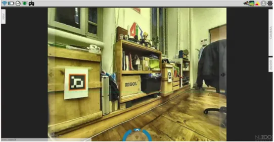
The provided ROS workspace includes most of the nodes and topics needed to start our work. In particular, there are nodes responsible for publishing sensors data, such as encoders, IMU, camera vision, laser scans and markers. Moreover, we have the nodes used to control the robot through the command velocity topics, via joy-pad or browser interface. The browser interface itself is also a useful piece of software, which allows the user to see the images provided by the two cameras and the recognized marker, and to

(19)

Figure 2.2: NuZoo web interface. The recognized marker is orange bordered.

manage the various minor functionalities such as speakers, lights and so on.

2.2.1 ROS topics

In this section we will describe the most relevant, for our purposes, ROS topics published and/or subscribed by the previously implemented nodes. They allow the ROS system to communicate both with sensors and actu-ators, by reading outputs and sending commands respectively. The topics are introduced with the name and the message type used.

• /r2p/encoder l and /r2p/encoder r, std msgs/Float32:

These topics, and all of the following ones which have a name starting with r2p/, are published by the r2p board, which manages most of the sensors. In particular, these topics publish as messages the number of ticks per second done by the left wheels (r2p/encoder l) and the right ones (r2p/encoder r). Every tick corresponds to a portion of spun wheel.

• /r2p/imu raw, r2p msgs/ImuRaw:

This topic contains the raw messages from the IMU, which include gyroscope, accelerometer and magnetometer. The r2p msgs/ImuRaw is a custom message type built by a three tridimensional vectors: angular velocity, linear acceleration and magnetic field. The names are self-explanatory enough and every vector has one compo-nent per axis: x, y, z. The values published represent the MEMS sensor register copy. In particular, the gyroscope has a 16 bit reading,

(20)

covering a range from -500 dps to +500 dps, with a sensitivity of 17.50 mdps per LSB and the accelerometer has a 12 bit reading, covering the range from −2g to +2g, that is about 1mg per LSB. The g here stands for the gravitational acceleration which measures about 9.81 m/s2

• /r2p/odom, geometry msgs/Vector3:

In this topic is published a very raw odometry, built in the board system. It is retrieved only by encoders data elaborations and is pub-lished as a vector of three elements in which the first and the second elements represent the position variation in meters (x and y) and the third element represents the orientation angle variation in radians.

• /nav cam/markers, nav cam/MsgMarkers:

In this topic is published the list of markers recognized by the robot in real time. Each marker is represented as a nav cam/MsgMarker mes-sage, which includes a numerical id of the marker (id), the name of the published marker frame (frame id) and its transform with the respect of the camera frame (pose), divided in position, as a tridimensional vector, and orientation, as a quaternion.

• /odom, nav msgs/Odometry:

In this topic is published the odometry, built by integrating the gyro-scope measurement in a ad hoc way. We improved this odometry for these project, as we will explain in ??. The nav msgs/Odometry mes-sage contains pose information, divided in position and orientation, and twist information, i.e. velocity, which is divided in linear and angular, both with the respective covariance matrices.

• /scanf, sensor msgs/LaserScan:

In this topic are published messages from the Hokuyo laser scanner, after being filtered by some outliers. The sensor msgs/LaserScan messages represent the collection of the distances at which an infrared ray beamed by the laser scanner has been intercepted by an obstacle.

2.2.2 Built-in navigation

The provided workspace includes different ways to teleoperate the robot. All of them always use the so called “laser bumper” which basically interrupts all forward movements in case of obstacle detected by laser scanner in a very

(21)

Figure 2.3: Ra.Ro. photograph from NuZoo website

close range. The teleoperation system operates in three ways: a manual one, an assisted one and a semi-autonomous.

Manual teleoperation

The manual teleoperation managed through the web application using a remote controller being plugged into a computer and connected to the robot via network. It is the simplest way and it is relies completely on human control.

Assisted teleoperation

The assisted teleoperation is managed via the web application interface which in this case can be runned even on mobile devices. It is Google street view inspired and allows to move the robot towards a specific spot by clicking or touching on the correspondent on-screen spot in the map besides its basic movements such as forward, backward and left and right rotation. The system cannot manage any obstacle in the trajectory. We can also consider as assisted teleoperation the one with the particular follow me marker. The operator must show the marker to the robot’s navigation cam and the robot it will try to keep the marker into the camera frame, following the person that holds it.

Semi-autonomous teleoperation

The most advanced navigation systems built into the robot consist in line following and in marker indication following. The first one consists in following colored line sticked or painted on the floor. It is possible to switch from one color to another. The second one consists in executing simple navigation tasks according to the recognition of a specific marker, which can be attached in sequence on walls creating, if needed, a patrol path.

(22)

Examples of a marker command can be to turn left 90◦, turn 180◦, keep the wall on your right. Moreover, a special marker is set on the recharging station and the robot can, under proper conditions, autonomously connect itself to the station after recognizing the marker, if desired.

None of these system implements a proper obstacle avoidance algorithm, nor a good odometry calculation. There is no mapping system, thus no localization is possible.

2.3 Platform purposes

As introduced at the beginning of this chapter, the full Ra.Ro. platform is designed to be a security guard, able to patrol parkings, supermarkets and so on. It has been already adapted by the producer company for other different purposes, usually starting from its simpler version, code name Geko, which is very similar to Ra.Ro. except for the cameras, which are attached directly to the robot base.

(23)

Chapter 3

Knowledge requirements

“Smirk : I like your spirit. I’ll do what I can. Of course... it’ll cost you. What have you got?

Guybrush : All I have is this dead chicken.

Smirk : That isn’t one of those rubber chickens with a pulley in the middle is it? I’ve already got one. What ELSE have you got?

Guybrush : I’ve got 30 pieces of eight.

Smirk : Say no more, say no more. Let’s see your sword. Guybrush : I do have this deadly-looking chicken.

Smirk : Yes, swinging a rubber chicken with big metal pulley in it can be quite dangerous... BUT IT’S NOT A SWORD!!! Let’s see your sword.”

The Secret of Monkey Island

3.1 State estimation

For a robot interacting with the environment it is important to retrieve information about the state of the environment around it and the state of the robot itself. This knowledge cannot be summarized into a unique hypothesis, in fact it is crucial to also have a characterization of the uncertainty of this knowledge [9].

We define the state of a robot as the values of specific variables needed to identify the robot and/or parts of it in a specific state space, for exam-ple velocity, position or orientation of a particular component. Most of the contemporary autonomous robots represent the possible states using proba-bility distributions in order to not rely only on a single “best guess”, but to have the possibility to update frequently the estimate of the state and the past states as well while required.

(24)

A well designed movable robot should be able to retrieve heterogeneous information given by different kind of sensors, in order to make the update of the possible states.

This is basically the definition of sensor fusion and in the following paragraph we are going to introduce the most used probabilistic techniques to estimate a state. These techniques are employed in different fields but on this essay we will focus only on robotic field.

3.1.1 Baysian state estimation

We define the belief of a state with the following formula:

bel(xt) = p(xt|z1:t, u1:t)

So the belief of a state in time t is defined as the probability to be in that state given the measurements z from the sensors and the known input values u until the time t.

To retrieve the measurement of the sensor at the t time is not very practical. In fact, the formula

bel(xt) = p(xt|z1:t−1, u1:t)

is more often used, in wich a posterior distribution represents the probability of each state given its prior, i.e. sensor readings and the controls until time t − 1. Hence this distribution is called prediction. From bel(xt) we can

obtain bel(xt) in recursive fashion, considering the first term as prior and

the second one the posterior. The most general form of the recursive state estimation is the Bayes filter, which is here reported.??

For each state variable we can divide its estimation into two steps.In the first one, the prediction, we estimate the state variable at time t given the ut and xt−1. In the second one, the innovation, the sensor readings zt are

used, combined with the previously calculated prediction. The mathematical formulation of the Bayes filter is given by

bel(xt) = ηp(zt|xt)

Z

x

p(xt|xt−1, ut)p(xt)dxt−1

which can be obtained:

• from the Bayes rule: P (B|A)P (A)_{P (B)} , together with the law of total prob-ability: P (A) =P

nP (A|Bn)P (Bn)

• assuming that the states follow a first-order Markow process, i.e. past and future data are independent if the current state is known: p(xt|x0:t−1) =

(25)

Algorithm 1 Bayesian filtering 1: _{function BayesFilter(bel(x}t−1), ut, zt) 2: for all x do 3: bel(xt) ← R xp(xt|xt−1, ut)p(xt)dx 4: bel(xt) ← ηp(zt|xt)bel(xt) 5: end for 6: return bel(xt) 7: end function

• assuming that the observation are independent of the given states, i.e. p(zt|x0:t, z1:t.u1:t) = p(zt|xt)

The generic Bayes filter algorithm is mostly impossible to use since the analytical representation of the multivariate posterior is usually difficult to retrieve. Moreover, the integrals involved in the prediction represent a very high computational effort.

The first practical implementation of the Bayesian filter for continuous domains was made by Rudolph E. Kalman, in 1960. The original formu-lation assumes that the belief distributions and measurement noise follow a Gaussian distribution and that system and observation models are linear [6]. Under these assumptions, the Kalman update equation yields the opti-mal state estimator, in terms of mean squared-error. The so called Kalman Filter (KF) is very important and it is still considered the state of the art in state estimation, especially its more generic version, the Extended Kalman Filters (EKFs), which admit in a sense the non-linearity of the system. The solution lies in Taylor series expansion applied to linearize the requested functions. These solutions are still widely employed today and are often the first choice in recursive state estimation. However, none of the KFs hold in the non-linear case. In particular, the EKFs can suffer from a poor approx-imation caused by the linearization of highly non-linear models affected by the propagation of the Gaussian noise.

In 1997, Simon Julier and Jeffery Uhlmann proposed the Unscented Kalman Filter (UKF) which, using the unscented transform for the lin-earization, can obtain better results in terms of accuracy, keeping the char-acterization of the error as Gaussian noise, which is usually reliable enough, and above all, easy to represent since the mean and the covariance give the full description of the distribution.

An alternative to the Kalman Filters is given by non-parametric filters. These ones does not rely on an analytic representation of the posterior prob-ability distribution, nor on parameters or statistics that can represent them.

(26)

A well-known approach is the particle filter, proposed by Gordon et Al. in 1993 [4]. The idea is to describe the posterior distribution in a Monte Carlo fashion, representing a possible state with a particle. The more particles are present in a certain region of the state space, the more that state is likely to be the real state. The advantage of this approach is that any kind of distribution can be represented in this way, but still problems exist. In particular we have to deal with a possible high dimension of the state space which carries the exponential growth of the number of particles needed to represent the probability distribution of the belief.

3.1.2 Graph-based State Estimation

For SLAM problem, in 1997, Lu and Milios developed and proposed a graph-based approach. In their formulation the nodes in the graph represent poses and landmark parameterizations. If a landmark is visible from a certain pose, then an edge linking the two poses is added. The state estimation problem consists in a maxi-likelihood optimization. Since every node and edge represents respectively poses and landmarks, the aim is to maximize the observations joint likelihood. This requires to solve a large non-linear, least-squares, optimization problem.

Graph-based approaches are considered to be superior to conventional EKF solutions, even though a more accurate research from the point of view of computational complexity is required in order to make them faster and thus more usable in on-line state estimation. The graph technique implies that not only the latest state can be estimated, but also the previous ones, making possible to continuously estimate the full robot trajectory.

An even wider generalization of the graph approach is the factor-graph, which is basically a hypergraph in which edges do not incide only between two nodes, but can possibly affect many of them. This comes up with a powerful tool in multi-sensor fusion problems, in particular it is appreciated the possibility to represent heterogeneous measurement, in sense of number of poses effected, maintaining a quite explicit design of the graph.

3.2 Odometry estimation

Odometry basically measures the distance traveled by a robot, or any kind of movable system, from an initial point, into the space in which it operates. It is crucial to have a good odometry estimation for many reasons, in particular for autonomous navigation. A good odometry estimation can be done only by retrieving and combining different sensor measurements, but certainly

(27)

the piece of information given by the wheels’ rotation is the base for the whole estimation, for every wheeled mobile robot.

3.2.1 Generic odometry

As mentioned before, the wheels’ rotation usually gives the most of the information about odometry, especially in the case in which an absolute pose measurement is not available, e.g. GPS sensor in indoor environment. As we are dealing with wheeled robots we can collapse our working space in a 2D plane, so estimate its odometry means indeed to estimate the posi-tion and the orientaposi-tion of the robot in this space. It follows that a three element vector (x, y, θ) is enough to represent this information. More pre-cisely the x and the y represent the two coordinate of the plane, considering the origin (0, 0) the initial position, and θ the rotation of the robot, with the respect of the initial orientation, around its vertical axis.

Each wheeled mobile robot (WMR) to be able to move must have a point around which all wheels follow a circular course. This point is known as the instantaneous center of curvature (ICC) or the instantaneous center of rotation (ICR). In practice it is quite simple to identify, because it must lie on a line coincident with the rotation axis of each wheel that is in contact with the ground. Thus, when a robot turns the orientation of the wheels must be consistent and a ICC must be present otherwise the robot cannot move.

If we could retrieve the sequence of the exact position variation of the robot (∆x, ∆y, ∆θ) at a good rate, the odometry would be simply the inte-gration of these measurement. These delta positions could be, if necessary, derived from the velocity along the axis.

Defined as v(t) the linear velocity in a t instant of time and ω(t) the angular velocity at the same time, can be generally retrieved the position and orientation of the robot at time t1 as follows

x(t1) = Z t1 0 v(t)cos(θ(t))dt y(t1) = Z t1 0 v(t)sin(θ(t))dt θ(t1) = Z t1 0 ω(t)dt (3.1)

In order to deal with concrete cases, namely discrete time, exist different integration methods. We will present three of the most common ones: Euler method, II order Runge-Kutta method and the precise reconstruction. For

(28)

(a) Euler method (b) Runge-Kutta method (c) Exact reconstruction Figure 3.1: Different integration methods results

these explanation we will use the relaxed notation xk = x(tk), vk = v(tk)

and so on, and we define Ts= tk+1− tk, namely the sampling period.

Euler method        xk+1= xk+ vkTscosθk xk+1= yk+ vkTssinθk θk+1= θk+ ωkTs (3.2)

This is the most simple integration method, but also the most subject to error in xk+1 and yk+1. θk+1 is exact in fact and it will be used also for

all the other integration methods, indeed. The whole system is correct for straight path. In general the error decreases as Ts gets smaller.

II order Runge-Kutta method

               xk+1 = xk+ vkTscos(θk+ ωkTs 2 ) xk+1 = yk+ vkTssin(θk+ ωkTs 2 ) θk+1= θk+ ωkTs (3.3)

Comparing with the Euler method, the II order Runge-Kutta one de-creases the error in computation of xk+1 and yk+1 using the mean value of

θk. Also in this case the smaller is sampling period Ts, the smaller is the

(29)

(a) TurtleBot (b) Khepera

(c) Robuter

Figure 3.2: Commercial differential drive robots

Precise reconstruction              xk+1= xk+ vk ωk (sinθk+1− sinθk) xk+1= yk− vk ωk (cosθk+1− cosθk) θk+1 = θk+ ωkTs (3.4)

Here is involved the instantaneous radius of curvature R = vk

yk. Note

that for ωk= 0 → R = ∞ the equation degenerate matching the Euler and

Runge-Kutta algorithms. The method is based on geometrical considera-tions.

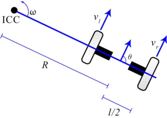
3.2.2 Differential drive odometry

The differential drive mechanism consist in two active wheels, rotating on a common axis, drove by two different motors. In addition one or more passive castor wheel(s) can support the robot stability without interfere with the robot kinematic. Many commercial robots adopts this kind of mechanism due the simplicity of implementation, the relative low cost and the com-pactness of the system. We can found it in TurtleBot, Khepera or Robuter. The whole robot motion is based on the difference in rotation velocity of the

(30)

Figure 3.3: Differential drive kinematics

two active wheels. The ICC lies on of course on the axis the wheels rotate around and the curve that the robot will follow depend on the position of this point with the respect of the middle point between the two wheels.[IMG]

The relationship between the wheels velocity vr and vl, the distance

be-tween the ICC and the midpoint of the wheels R and the angular velocity of the robot ω is given by the following

ω(R + l 2) = vr

ω(R − l 2) = vl where l is the distance between the 2 wheels.

We are actually interested in retrieve R and ω” from the velocities, which are usually available data given by the encoders, and l which is a fixed parameter. So the formulas are:

R = l(vr+ vl) 2(vr− vl)

ω = vr− vl l

(3.5)

It is interesting to analyze a couple of special case. When vr = vl then

R = inf, which means that the robot is moving in a straight line, is not curving. When vl = −vr then R = 0, which means that the robot is only

rotating around the vertical axis passing through the midpoint between the wheels.

(31)

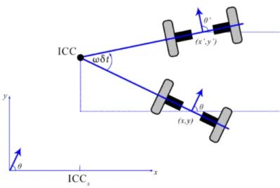
Figure 3.4: Differential drive robot motion from pose (x, y, θ) to (x0, y0, θ0)

Since the differential drive structure is non-holonomic, is not possible to do, for example, a lateral movement or any other kind of displacement not represented by the previous equations.

The position (x0, y0, θ0) in a particular instant of time is given by the computation on the previous (x, y, θ) and the time span ∆t between the two positions    x0 y0 θ0   =    cos(ω∆t) −sin(ω∆t) 0 sin(ω∆t) cos(ω∆t) 0 0 0 1       x − ICCx y − ICCy θ   +    ICCx ICCy ω∆t   

Where ICCx and ICCy are the coordinate computed as follows:

ICC = (x − Rsin(θ), y + Rcos(θ))

The specific case for the odometry calculation in differential drive, ac-cording with 3.1 is x(t1) = 1 2 Z t 0 (vr(t) + vl(t))cos(θ(t))dt y(t1) = 1 2 Z t 0 (vr(t) + vl(t))sin(θ(t))dt θ(t) = 1 l Z t 0 (vr(t) − vl(t))dt (3.6) 31

(32)

3.2.3 Skid-steering odometry

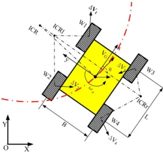
The skid-steering mechanic tries to maintains the simplicity and compact-ness of the differential drive, improving in the meanwhile the robustcompact-ness of the model. It consists in four wheels that we can divide in a pair on the left, front and rear, and a pair on the right, again front and rear. Each couple of wheels is driven by one motor, located in the middle of the front and rear wheel. These two wheels are usually connected by a transmission belt or a chain. Each motor allows to rotate the pair of wheels connected at with the same velocity.

Skid-steering compactness and the high maneuverability, in addition to the higher robustness, with the respect of the differential drive, makes this kind of mechanic an optimal choice for different purposes. This mechanic, indeed, offer a good mobility on different terrains, not only indoor ones, but also outdoor, because one of the advantages is the possibility of mount tracks for the terrains that require them, without changing the whole mechanic.

Unfortunately the drawback is a more complex kinematics because the pure rolling and no-slip assumption, that was possible to use for the differ-ential drive case, is no more an option because the wheels must slip during a curve. This implies a hard to predict motion, given the velocity input. Other disadvantages are an energy inefficient motion and a fast tires’ consumption, caused by the slippage indeed.

Wang et al. help to partially resolve the problem of the complex skid-steering kinematic proposing an approximation to the differential drive one. It is based on three assumption:

(i) the mass center of the robot is located at the geometric center of the body frame

(ii) the two wheels of each side rotate at the same speed (wf r = wrr and

wf l = wrl)

(iii) the robot is running on a firm ground surface, and four wheels are always in contact with the ground surface

Then considering the figure and the deriving the Equations ?? we obtain

   vx vy wz   = f " wlr wrr # (3.7)

where v = (vx, vy) is the vehicle’s translational velocity with respect to

its local frame, wz is its angular velocity, r is the radius of the wheels and

(33)

Figure 3.5: Skid-steering platform

During robot turn there are different ICRs: ICRl, ICRr and ICRG,

that are respectively of the left-side tread, right-side tread, and the robot center of mass. We define the coordinates of the ICRs respect to the local frame as (xl, yl), (xr, yr) and (xG, yG). All the treads share the same angular

velocity ωz, so these equations follows

yG= vx wz (3.8) yl= vx− wlr wz (3.9) yr= vx− wrr wz (3.10) xG= xl= xr= − vy wz (3.11)

from (??) to (??) the generic odometry kinematic (??) can be repre-sented as:    vx vy wz   = Jw " wlr wrr # (3.12) 33

(34)

Figure 3.6: Skid-steering to differential drive equivalence

Where Jw depends on IRCs coordinates and is defined as follows:

Jw = 1 yl− yr    −yr yl xG −xG −1 1    (3.13)

If the robot is symmetrical, then the ICRs will lie symmetrically on the x-axis, and will be xG = 0 and y0 = yl= −yr. The Jw matrix be rewritten

as: Jw = 1 2y0    y0 y0 0 0 −1 1    (3.14)

So the velocities defined in (??) can be defined, for the symmetrical model, as follows:          vx= vl+ vr 2 vy = 0 wz= −v_l+ vr 2y0 (3.15)

and from (??) we can get the instantaneous radius of the path curvature:

R = vG wz

= vl+ vr −vl+ vr

(35)

The ratio of sum and difference of left and right wheels’ linear velocities can be defined as a variable λ

λ = vl+ vr −v_l+ vr

and (3.16) becames

R = λy0

A similar approach is used in Mandow’s work, in which an IRC coeffi-cient χ is defined as:

χ = yl− yr

B =

2y0

B , χ ≥ 1 (3.17)

χ represents the approximation from the differential drive kinematic. We can notice that when χ is equal to 1 there is no slippage and the skid-steering model coincide with the differential drive. It implies that we can use the differential drive model to approximate the skid-steering one, working on the χ variable. In particular the skid-steering coincide with a differential drive with a larger span between the left and right wheels as shown in Figure. This is a very useful method and will be very appreciated for our work.

3.3 Sensor fusion framework

Since, as mentioned before, the pure kinematics equations are actually just an approximation of the real world, they are not enough to retrieve the correct odometry of a robot with a satisfying precision. This is why the multi-sensor fusion is required. Here we introduce the framework used to make this process in a way possible to set up.

3.3.1 ROAMFREE

The acronym ROAMFREE stays for Robust Odometry Applying Multi-sensor Fusion to Reduce Estimation Errors. The main aim of the framework is to offer a set of mathematical techniques and to perform sensor fusion in mobile robotics, focusing on pose tracking and parameter self-calibration. The main goals of the project include ensuring that the resulting software framework can be employed on very different robotic platforms and hardware sensor configurations and that it can be easily tuned to specific user needs by replacing or extending its main components.

In ROAMFREE the information fusion problem is formulated as a fixed-lag smoother whose goal is to track not only the most recent pose, but all

(36)

the positions and attitudes of the mobile robot in a fixed time window: short lags allow for real time pose tracking, still enhancing robustness with respect to measurement outliers; longer lags allow for online calibration, where the goal is to refine the available estimate of sensor parameters.

The system is based on a graph-based approach. In particular a factor graph is generated. This graph keeps the probabilistic representation of the pose retrieved by the sensor fusion measurements, the estimated sensor parameters and the sensor error models. All the modules interact in some way with this graph, for example to update it with new measurements or new estimated poses. The factor graph is designed to allow an arbitrary number of sensors, even if they work at different rates, without a predictable rate or producing obsolete data.

The framework implements a set of logical sensor, which are indepen-dent from the actual hardware that produce the measurement. For example an odometry measurement can be retrieved from a laser scanner elabora-tion or an wheels’ encoders one, but both can be properly setted up as a logical GenericOdometer sensor. Each logical sensor is characterized by a parametric error model specific for its domain. This means that we must initialize the sensors passing the specific parameters for that sensor. For example a DifferentialDriveOdometer requires the wheels radius and the wheels distance, expressed in meters. Another required parameter needed to properly set up a sensor is its position and orientation with the respect of the tracked base frame, in order to properly use the information retrieved. For example the camera sensor, possibly used to retrieve markers positions, must be properly set in order to calculate the exact transformation between the seen marker and the base frame.

The ROAMFREE’s modularity and its ROS implementation make it a very powerful tools for sensor fusion purposes and the other side aims. Unfortunately we had to deal with a lack of documentation which made the development of a stable ROS node quite hard.

Factor graph filter As mentioned before the core of ROAMFREE lies in the factor graph filter. We already written about the important features of graph-based approaches in paragraph ?? in a general way. The most rel-evant advantage is the possibility of menage high-dimensional problems in relatively short time. The graph holds the full joint probability of sensor readings given the current estimate of state variables, representing its factor-ization in terms of single measurement likelihoods. Each node of the graph contains a the pose of the robot and the sensors’ calibration parameters, i.e. gains, biases, displacement or misalignments. The nodes are generated by

(37)

Figure 3.7: An instance of the pose tracking factor graph with four pose vertices ΓW O(t)

(circles), odometry edges eODO(triangles), two shared calibration parameters vertices

kθand kv(squares), two GPS edges eGP S and the GPS displacement parameter S (O) GP S

new measurements, represented as hyper-edges (factors) connecting one or more nodes, depending on their order. For example a velocity measurement connects two nodes since it need one integration to retrieve a position; an acceleration needs three nodes because the twice integration required.

One, and only one, of the available sensors must be chosen as architecture master sensor, and a good practice is to choose an odometry sensor to play this role, because it has usually a high rate and it is the one that gives a hopefully good starting point for the optimization process. Once the master sensor measurement is collected, an initial guess of the new pose is made and then begins a non-linear optimization process, using also the other measurement retrieved in the meanwhile. It can happens that sensor reading are late for low rate, connection problems or in general are not available. In these cases, if the available once are not sufficient to generate a pose, the measurement handling is delayed until enough data are available.

The new node generation is based on a fixed-lag window. It means that only nodes contained in these time span are considered for the following pose. Older nodes and factors, since are no more used, are deleted. In order to avoid high loss of information older nodes and factors can be marginalized, keeping the information they used to holds in a new generated factor.

We can resume the factor-graph advantages here:

• Flexible with the respect of sensors’ nature and number. The mod-ularity of the system allows to manage all the inserted sensors in an independent and uniform way, by means the abstract hyper-edges

(38)

terface, as they are inserted into the graph.

• Sensors can be, if necessary, turned on and off during the process. The factors’ management is asynchronous, so they can be added into the graph as soon as new reading are available.

• Possible to deal with out-of-order measurements. If an old informa-tion is received, according to its time stamp, it will not be simply discarded, but will be created an appropriate factor, connecting the nodes interested by and updating and refining them.

• The quality of the estimation is higher and, in certain circumstances, faster than traditional filters, such as EKFs [8].

• The high degree of sparsity of the considered information fusion prob-lem is explicitly represented and can be exploited by inference algo-rithms. Indeed in our case a factor may involve up to three robot poses; moreover, it is difficult to imagine a robot employing much more than ten sensors for pose estimation, implying that each pose is incident to a limited number of factors.

Error models For each logical sensor model an error model definition is needed. All of these ones start from a common definition

ei(t) = ˆz(t; ˆxSi(t), ξ) − z + η (3.18)

where hatxSi(t) is the extended state for the sensor frame Siin which are

represented the position and the orientation of the frame with the respect of the world frame, its position and orientation at time t; ξ represents the vector of the parameters relative to that sensor and ˆz(t; ˆxSi(t), ξ)) is a predictor

measurement computed as a function of the previously defined parameters and the incident nodes. z is the real sensor output and η is the zero-mean Gaussian noise representing the measurement uncertainty. It is evident that the more the prediction is accurate, even equal to z, the more the error is near to 0, net of the Gaussian noise.

The equation that describes the actual error depends on the type of measurement considered. We can distinguish five classes:

(i) absolute position and/or orientation (e.g. GPS)

(ii) linear and/or angular velocity in sensor frame (e.g. gyroscope)

(39)

Figure 3.8: ROAMFREE estimation schema

(iv) vector field in sensor frame (e.g- magnetometer)

(v) landmark pose with respect to sensor (e.g. markers)

Moreover the other thing that characterize the sensor in ROAMFREE is the parameter’s vector ξ, which includes gain, bias and other specific parameters according to the sensor class. These parameters sometimes are easy to retrieve from sensors’ specifications or from observation, but often they need an accurate tuning to let everything works well.

An even more attention is required for covariance matrix setup. Indeed the factor graph wants this matrix as input in measurement update, in addition to the measurement itself and the sensor name. The covariance matrix can be even different according to the actual measurement, of course always being of the right dimension. Changing the value of the matrix means change the reliability of a sensor. In other words if two measurement indicate two conflicting outputs the system will trust more the one with a lower covariance.

A convenient feature is the outlier management made through the ro-bust kernel technique. It consist in setting a threshold in the measurement domain. If this threshold is exceeded, in module, the error model of the sensor, for that measurement, becomes linear instead of quadratic, which means that it is less involved in the following computation. It is useful to manage with errors that can sometimes occur in data retrieving.

Optimizations The optimization algorithms implemented in ROAMFREE are Gauss-Newton and Levenberg-Marquardt. Both of them require a prob-lem formulated as non-linear, wighted and least-squares optimization and here will discuss about how it is done. Consider the error function ei(xi, η)

(40)

associated to the i-th edge of the hyper-graph and defined as (??). We can approximate the error function as ei(xi) = ei(xi, η)|η=0since ei is a random

vector. It can involve non-linear dependencies with respect to the noise, so its covariance Ση is computed by means of linearization, i.e.:

Σei = Ji,ηΣηJ

T

i,η|xi=˘xi,η=0 (3.19)

where Ji,η is the Jacobian of ei with respect to η evaluated in η = 0 and

in the current estimate ˘xi. The covariance matrix Sigmaη is the one we

mentioned before and here is where it is involved in the optimization. A negative log-likelihood function can be associated to each edge in the graph, which stems from the assumption that zero-mean, Gaussian, noise corrupts the sensor readings. Omitting the terms which does not depend on xi, for the i-th edge this function reads as:

L_i(xi) = ei(xi)Ωeiei(xi) (3.20)

where Ωei = Σ

−1

ei is the information matrix of the i-th edge. The solution

for the information fusion problem is given by the assignment for the state variables such that the likelihood of the observations is maximum,

P = argmin x N X i=1 L_i(xi) (3.21)

It is possible to observe that this is a non-linear least-squares problem where the weights are the information matrices associated to each factor. If a reasonable initial guess for x is known, a numerical solution for P can be found by means of the popular Gauss-Newton (GN) or Levenberg-Marquardt (LM).

3.4 Simultaneous Localization and Mapping (SLAM)

With simultaneous localization and mapping (SLAM) is meant the building of a map while the robot locate itself into the map that is being created. The SLAM can be considered a preliminary phase in which the robot create the map and then it will use it for the autonomous navigation, or can be contextual to the autonomous navigation. It is important to point out that it does not matter if the robot, during the SLAM phase, is human controlled or not. The first localization guess is given by the odometry, but, as mentioned in section (??), it accumulates error as long as the robot moves. A good odometry estimation is desirable for the SLAM problem, but the error given by the odometry can be corrected using world references observed through

(41)

laser scanner(s), camera(s) (Visual SLAM) or similar sensors. It follow that the observation should be done in an environment as static as possible, even if SLAM frameworks can deal with mobile objects. Moreover the localization makes sense if it is made with respect of a map, but if the map is being made is evident the possible problem that can shows up. For sure SLAM must be done in recursive way and this is one of the main reason why is a so complex task. From a probabilistic point of view, there are two main forms of SLAM. One is known as the online SLAM problem: it involves estimating the posterior over the momentary pose along with the map:

p(xt, m|z1:t, u1:t) (3.22)

Where xt is the pose time at time t, m is the map and z1:t and u1:t are

the measurements and controls, respectively. This problem only involves the estimation of the variables that exist at time t. Many algorithms for the online SLAM problem are incremental: they discard past measurements and controls once they have been processed.

The second SLAM problem is called the full SLAM problem. Here we want to calculate a posterior over the entire path x1:t along with the map,

instead of just the current pose xt:

p(x1:t, m|z1:t, u1:t) (3.23)

Instead of computes the state incrementally as in online case, here the se-quence of states is computed one time.

Regardless of the method used to implement a full or online SLAM, the algorithm must follows these steps:

(i) Landmarks detection: the robot must recognize some feature from the environment, called landmarks. For a 2D map, horizontal LIDAR are the most common sensor used for this kind of task. Angles, edges, particular shapes are good candidates to be detected as landmark.

(ii) Data association: once the landmark is been detected, it must be matched with an possibly existing landmark into the map. It can be a hard task because a single feature can match with many, growing exponentially as long as the map grows.

(iii) State estimation. It takes observations and odometry to reduce errors. The convergence, accuracy, and consistency of the state estimation are the most important properties. Thus, the SLAM method must main-tain the robot path and use the landmarks to extract metric constraints to compensate the odometer error.

(42)

Figure 3.9: The image represent the topics subscribed and published by the mapping node, independently by the exact mapping system used

The major difficulties of SLAM are the following:

• High dimensionality: since the map dimension always grows when the robot explores the environment, the memory requirements and time processing of the state estimation increase. Some submapping techniques can be used to reduce these consumption, at the cost of a worse performance

• Loop closure: when the robot revisits a past place, the accumulated odometry error might be large. Then the data association and land-mark detection must be effective to correct the odometry. Place recog-nition techniques are used to cope with the loop closure problem.

• Dynamics in environment: state estimation and data association can be confused by the inconsistent measurements in the dynamic ronment. There are some methods that try to deal with these envi-ronments.

We will focus on 2D SLAM, using a laser scanner as sensor and related laser scans measurements. In general the aim of a SLAM framework is to collect the laser scans and try to associate them in one occupancy grid map. Then, if following scans match with the memorized map, the position will be corrected according to this match, hopefully improving the localization estimation. The more various the environment is, the more the localization is easy, because the probability to deal with a potential ambiguity is lower.

3.4.1 Gmapping

Gmapping is the most widely used laser-based SLAM package in robots worldwide. The algorithm has been proposed by Grisetti et al.in 2007 and it is a Rao-Blackwellized Particle Filter SLAM approach.

We mentioned the Particle Filter in section ?? and here we will describe RBPF, which is an optimized version for the SLAM problems.

(43)

Algorithm 2 Improved RBPF for map learning

Require:

St−1, the sample set of the previous time step

zt, the most recent laser scan

ut−1, the most recent odometry measurement

Ensure:

St, the new sample set

St= { }

for all s(i)_t−1∈ St−1do

hx(i) t−1, w (i) t−1, m (i) t−1i = s (i) t−1 //Scan − matching x0 (i)_t = x(i)_t−1⊕ u_t−1 ˆ

x(i)_t = argmax_xp(x|m(i)_t−1, zt, x0 (i)t )

if ˆx(i)_t = failure then x(i)_t ∼ p(xt|x(i)t−1, ut−1)

w(i)_t = w(i)_t−1· p(zt|m(i)t−1, zt, x0 (i)t )

else

//Sample around the mode for all k = 1 to K do

xk∼ {xj| |xj− ˆx(i)| < ∆}

end for

//Compute Gaussian proposal µ(i)_t = (0, 0, 0)T

η(i)= 0

for all xj∈ {x1, . . . , xK} do

µ(i)_t = µ(i)_t + xj· p(zt|m(i)t−1, xj) · p(xt|x(i)t−1, ut−1) η(i)_{= η}(i)_{+ p(z}

t|m(i)t−1) · p(xt|x(i)t−1, ut−1)

end for µ(i)_t = µ(i)_t /η(i)

Σ(i)_t = 0

for all xj∈ {x1, . . . , xK} do

Σ(i)_t = Σ(i)_t + (xj− µ(i)t )(xj− µt(i))T· p(zt|m(i)t−1· p(xt|x(i)t−1, ut−1)

end for Σ(i)_t = Σ(i)_t /η(i) //Sample new pose x(i)_t ∼ N (µ(i)t , Σ

(i) t )

//U pdate importance weights w(i)_t = w(i)_t−1· η(i)

end if // U pdate map

m(i)_t = integrateScan(m(i)_t−1, x(i)_t , zt) // U pdate sample set

S_t= St∪ {hx(i)t , w (i) t , m (i) t i} end for Nef f= 1 ΣN i=1( ˜w(i))2 if Nef f< T then St= resample(St) end if

We can start from (3.23) and factorize it as:

p(x1:t, m|z1:t, u1:t) = p(m|x1:t, z1:t)p(x1:t|z1:t, u1:t−1) (3.24)

This factorization allows to first estimate only the trajectory of the robot and then to compute the map given that trajectory. In particular p(m|x1:t, z1:t)

can be easily computed using “mapping with known poses” since x1:t and

z1:t are known.

The RBPF occupancy grid SLAM works as follows:

If new control data ut from the odometry and a new measurement zt

(44)

form the laser scanner is available:

1. Determine the initial guess x0_t(i), based on ut and the pose, since the last

filter t update xt−1 has been estimated.

2. Perform a scan matching algorithm based on the map m(i)_t−1 and x0_t(i). If the scan matching fails, the pose x(i)_t of particle i will be determined according to a motion model, otherwise the next two steps will be per-formed.

3. If the scan matching is successfully done, a set of sampling points around the estimated pose ˆx(i)_t of the scan matching will be selected. Based on this set of t poses, the proposal distribution will be estimated.

4. Draw pose x(i)_t of particle i from the approximated Gaussian ditribution of the improved proposal distribution.

5. Perform update of the importance weights.

6. Update map m(i) of particle i according to x(i) and zi.

The more detailed RBPF algorithm pseudo-code can be read in (??). The author proposes a way to compute an accurate distribution by taking into account both she movement of the robot and the most recent observa-tions. This decreases the uncertainty about the robot’s pose in the prediction step of the particle filter. As a consequence, the number of particles required decreased since the uncertainty is lower, due to the scan matching process, improving the performance.

3.4.2 Cartographer

Another possible approach for SLAM problem is using graph-based meth-ods. These ones use optimization techniques to transform the SLAM prob-lem into a quadratic programming probprob-lem. The historical development of this paradigm has been focused on pose-only approaches and using the landmark positions to obtain constraints for the robot path. The objective function to optimize is obtained assuming Gaussianity. Since this meth-ods are based on a factor graph, they are able to remember better the old sub-maps and the old localization and thus results more accurate respect to other approaches.Their main disadvantage is the high computational time they take to solve the problem, so they are usually suitable to build maps off-line.

(45)

Google’s Cartographer provides a real-time solution for indoor and out-door mapping. The system generates submaps from the matching of the most recent scans at the best estimation position, which is assumed to be accurate enough for short periods of time. Since the scan matching works only on submaps the error of the pose estimation in the world frame eventu-ally increase. For this reason the system runs periodiceventu-ally a pose optimiza-tion algorithm. When a submap is considered finished, no more scans are added to it and it takes part in scan matching for loop closure. If the robot estimated pose is close enough to one or more processed submap, the algo-rithm runs the scan matching between the incoming laser scans and those maps. If a good match is found it is added as a loop closing constraint to the optimization problem. By completing the optimization every few sec-onds, the loops are closed immediately when a location is revisited. This leads to the soft real-time constraint that the loop closure scan matching has to happen quicker than new scans are added, otherwise it falls behind noticeably. This has been achieved by using a branch-and-bound approach and several precomputed grids per finished submap.

3.5 Localization

As mentioned before, robot localization is the problem of estimating a robot’s pose relative to a map of its environment. It has been defined as one of the most fundamental problems in mobile robotics [3].

We can recognize different levels of localization problems. The localiza-tion tracking is the simplest one; the robot starts from a known posilocaliza-tion and the localization aim is to correct the hopefully small odometry errors. A more challenging problem is the global localization problem; the robot must localize itself without a given initial position. An even more difficult problem is the kidnapped robot problem; it can happen that an even well localized robot is moved, with no information about this transportation, to a different location. It can seems a similar problem to the second one, but here we can not trust a measurement as consistent with a previous one, be-cause the loss of information during the unexpected movement. Moreover it is useful to correct very bad localization problems.

In other words the localization problem consist in identify an appropri-ate coordinappropri-ate transformation between the global frame, which is fixed and integral with the map, and the robot frame. Then a detected object from the robot point of view can be, in turn, transformed with the respect of the global frame by coordinate transformation.

In robot localization the state xt of the system is the robot position,

(46)

Algorithm 3 Adaptive variant of Monte Carlo Localization

1: _{procedure AMCL(X}t−1, ut, zt, m)

2: X_t= Xt= 0

3: for all m := 1 toM do

4: x(m)_t = SampleMotionModelOdometry(ut, x(m)_t−1) 5: w(m)_t = MeasurementModel(zt, x(m)t , m); 6: X_t= Xt− hx(m)t , w (m) t i 7: wavg = wavg+ 1 Mw (m) t 8: end for

9: wslow = wslow+ αslow(wavg− wslow)

10: wf ast= wf ast+ αf ast(wavg − wf ast)

11: for all m := 1 to M do

12: with probability max(0.0,1.0 - wf ast

wslow) do 13: add random pose to Xt

14: else

15: draw i ∈ {1, . . . , N } with probability ∝ x(m)_t

16: add x(i)_t to Xt

17: end with

18: end for

19: return Xt

20: end procedure

which, for the two dimensional mapping, is typically represented as a three dimension vector xt= (x, y, θ) in which x and y indicate the position of the

robot in the map plane, and θ the angle formed by the robot orientation. The state transition probability p(xt|xt−1, ut−1) describes how the robot position

changes, given the previous position xt−1and the new sensors’ measurements

ut−1. The perceptual model p(zt|xt) describes the likelihood of making the

observation ztgiven that the robot is at position xt.

3.5.1 Adaptive Monte Carlo Localization (AMCL)

The Adaptive Monte Carlo Localization (AMCL) is a method to localize a robot in a given map. It is an improved implementation of particle filter. The word “adaptive” means that the number of particle used for the Monte Carlo localization is not fixed, but changes according to the situation. This number of particle is retrieved using the KLD-Sampling (Kulback-Leibler-Divergence) [5] [7]. The AMCL algorithm is here reported [??]. It requires the set of particles of the last known state Xt−1 and the control data utfor

(47)

the prediction; the measurement data zt and the map m for the update.

The algorithm returns the new status as a set of particles Xt. This filter

implementation is able to deal with the global localization problem, the localization problem and the kidnapping problem. The AMCL is flexible with the respect of the resampling technique, it means that an arbitrary one can be used. Another advantage is that AMCL is able to recover from localization errors by adding some random particles to the Xt set, after a

specified decade (lines 15 and 16 of ??). An AMCL ROS package is available [1] and a lot of robots uses this package for the localization since it provides a good configuration parameter suite.

3.6 A note on ROS reference system

Developers of drivers, models, and libraries need a share convention for co-ordinate frames in order to better integrate and re-use software components. Shared conventions for coordinate frames provides a specification for devel-opers creating drivers and models for mobile bases. Similarly, develdevel-opers creating libraries and applications can more easily use their software with a variety of mobile bases that are compatible with this specification. In this chapter we will explain the reference frames that should be used for a localization system, according to the ROS standard [?].

Coordinate frames

base link The coordinate frame called base link is rigidly attached to the mobile robot base. The base link can be attached to the base in any arbitrary position or orientation; for every hardware platform there will be a different place on the base that provides an obvious point of reference. A right-handed chirality with x forward, y left and z up is preferred.

odom The coordinate frame called odom is a world-fixed frame. The pose of a mobile platform in the odom frame can drift over time, without any bounds. This drift makes the odom frame useless as a long-term global reference. However, the pose of a robot in the odom frame is guaranteed to be continuous, meaning that the pose of a mobile platform in the odom frame always evolves in a smooth way, without discrete jumps. In a typical setup the odom frame is computed based on an odometry source, such as wheel odometry, visual odometry or an inertial measurement unit. The odom frame is useful as an accurate, short-term local reference, but drift makes it a poor frame for long-term reference.

(48)

map The coordinate frame called map is a world fixed frame, with its Z-axis pointing upwards. The pose of a mobile platform, relative to the map frame, should not significantly drift over time. The map frame is not continuous, meaning the pose of a mobile platform in the map frame can change in discrete jumps at any time.

In a typical setup, a localization component constantly re-computes the robot pose in the map frame based on sensor observations, therefore elim-inating drift, but causing discrete jumps when new sensor information ar-rives.

The map frame is useful as a long-term global reference, but discrete jumps in position estimators make it a poor reference frame for local sensing and acting.

earth The coordinate frame called earth is the origin of ECEF (earth-centered, earth-fixed) [?].

This frame is designed to allow the interaction of multiple robots in differ-ent map frames. If the application only needs one map the earth coordinate frame is not expected to be present.

Relationship between Frames

The relationship between coordinate frames in a robot system can be rep-resented as a tree since each coordinate frame can have a parent coordinate frame and an arbitrary number of child coordinate frames. Thus, the frames described before are attached as follows:

Figure 3.10: The tree frame representation.

The map frame is the parent of odom, and odom is the parent of base link. Although intuition would say that both map and odom should be attached to base link, this is not allowed because each frame can only have one parent.

Frame Authorities

The transform from odom to base link is computed and broadcast by one of the odometry sources.

(49)

The transform from map to base link is computed by a localization component. However, the localization component does not broadcast the transform from map to base link. Instead, it first receives the transform from odom to base link, and uses this information to broadcast the trans-form from map to odom.

The transform from earth to map is statically published and configured by the choice of map frame. If not specifically configured a fallback position is to use the initial position of the vehicle as the origin of the map frame. If the map is not georeferenced so as to support a simple static transform the localization module can follow the same procedure as for publishing the estimated offset from the map to the odom frame to publish the transform from earth to map frame.

(50)

(51)

Chapter 4

Navigation system for the

Ra.Ro.

“Guybrush: Van Winslow, head to Isle of Ewe!

Van Winslow: Please, sir, I think we should hit land first! Guybrush: Isle of Ewe... It sounds like ”I Love You”. Nice joke. Van Winslow: [Disappointedly] Yes, sir, joke...”

Tales of Monkey Island - The Siege of Spinner Cay

4.1 Navigation system overview

As we mentioned before, Ra.Ro. has already a kind of “autonomous” nav-igation system. It is based on line following and marker recognition, used as indication giver, such as “turn left”, “keep right”, “follow me” and so on. The system is quite reliable, if we accept the fact that we must attach in some way markers on walls and/or lines on the floor, and we are sure that the robot will not deal with movable or unpredicted obstacles, but it is very far from a real autonomous navigation. It is not possible, for example, to indicate any point on a map and expect that the robot will reach that point. So, our aim was to reach a solution at least reliable as the previous one, but more powerful. Ra.Ro. is ROS based, so the most logic approach was to implement the ROS navigation stack, and to work around it. The best advantage from this approach is the modularity of the system, and here follows the explanation of the modules we used in our project:

(52)

Figure 4.1: The ROS standard navigation stack schema

Odometry source

The odometry source provides the estimated robot position with respect to the starting pose. The easiest way to provide this data is to use the wheel encoder, but it is usually very imprecise because the slippage of the wheels, different floors friction, small obstacles that let the wheel rotate without robot movement, imprecise sensor itself and so on. So, to have a better odometry source is a good choice to use a multi-sensor fusion system, and it is basically most of the work of this thesis.

We compared a custom source developed manually integrating gyroscope and raw odometry provided by the wheels’ encoders and two factor graph filters built using the ROAMFREE framework; the first one using IMU sensor and encoders, and the second one using, in addition, the markers recognition.

Sensor sources

The sensor source is used by the navigation stack for mapping and for localization inside the mapped environment. It must generate PointCloud or LaserScan messages. In our case, since we mount a Hokuyo Laser scanner, we used this one as sensor source. A future work on this project could add as sensor source a module that can extrapolate point cloud from cameras.

Sensor transforms

For each sensor is necessary to provide a transform between the base frame and the sensor frame itself. The transformation must be published as a TF message and in our case is the static transform between the base-frame and the laser-frame.

(53)

Amcl

This module is optional. The Adaptive Monte Carlo Localization ap-proach uses a particle filter to track the pose of the robot against a known map (see map server, the following module). It corrects the robot position, estimated by the odometry system, moving the odom frame with the respect of the map frame. The less is the error in odometry estimation, the less the amcl module have to correct the position of the odom frame. During the initial phase, in which the robot doesn’t have to navigate autonomously, the amcl module can be missing.

Map server

As the amcl module, the map server is optional because is used in the autonomous navigation phase. It consists in a map previously collected or created.

Global Costmap and Global Planner

The global costmap carries the information about the obstacles in the map. It is possible to set up an inflation radius which represents a security distance that the robot must keep from the walls and other objects. These pieces of information are associated with a cost, and the global planner uses this cost information to find the most efficient path to reach a goal into the whole map.

Local Costmap and Local Planner

The local costmap is similar to the global one, but instead of deal with the whole map, is localized in a scrolling window around the robot. It is used to modify the global path according to unexpected obstacles, not included in the provided map. The local planner generates a modified path that should not deviate too much from the global one, according to the costs provided by the local costmap.

Base controller

The Twist messages outputted from the local planner are sent to the base controller. These messages represent the velocity that the robot should have to follow the generated path. The base controller is the module that interpret these messages and convert them into actual robot movement controlling the wheels’ speed.