Multiscale analysis of a HCN4 channel double mutation in a human sinoatrial computational model

(1)

A

LMA

M

ATER

S

TUDIORUM

· U

NIVERSITÀ DI

B

OLOGNA

S

CUOLA DI INGEGNERIA E ARCHITETTURA

C

ORSO DI

L

AUREA

M

AGISTRALE IN

I

NGEGNERIA

B

IOMEDICA

(LM)

T

ESI IN

M

ODELLI E

M

ETODI PER LA

C

ARDIOLOGIA

C

OMPUTAZIONALE

LM

Multiscale analysis of an HCN4 channel

double mutation

in a human sinoatrial computational model

Relatore:

STEFANO SEVERI

Correlatori:

FILIPPO CONA

ALAN FABBRI

Candidato:

EUGENIO RICCI

S

ESSIONE

III

A

NNO

A

CCADEMICO

2018/2019

(2)

(3)

Abstract

The Double Mutation (DM) I479V/A485E has been reported (Servatius et al., 2018) to determine a loss of function of the funny current (If), which is a key player of the onset of the action potential in the Sinoatrial Node (SAN). Thus, the DM can result in bradycardia. This work presents a multiscale study that links the DM (i.e. genotype) to the bradycardia (i.e. phenotype). To do this, first a tool to display and analyse electrophysiological data was developed. Thanks to it, the de-crease in If conductance was quantified and used as an input for a computational model of a human SAN cell. The simulation of the action potential of this model gave a Cycle Length (CL) of 1019 ms (compared to 814 ms of the Wild Type con-dition, +20.1 %). After this, a 1D and 2D model of the SAN were implemented, in order to test the behaviour of more complex systems (fibre and tissue), since these can show phenomena not present at the channel or single cell level. Several values of cellular heterogeneity (σ ) and coupling (ρ) were considered, in order to investigate the most physiologic degree of these properties. This was assessed relying on the most realistic results obtained for CL, Action Potential Amplitude (APA) and Conduction Velocity (CV). The results show that:1) increasing σ leads to shorter mean CLs and wider CL and APA distributions; 2) increasing ρ pro-vides wider CL and APA distributions, whereas their mean values are the highest for ρ = 1000 MΩ · m. A complete synchronization is therefore a trade-off be-tween σ and ρ; 3) for physiological values of σ (0.1873) and ρ (∼ 100 MΩ · m) cells manage to synchronize their pacing frequency and show a conduction veloc-ity similar to that reported in literature (∼ 11 cm/s) in both 1D and 2D models. This is true for both WT and DM but, in the last case, the mean CL is significantly shorter. This fact proves the detrimental effect of these mutations: in 2D, the heart rate drops from 75.6 bpm (WT) to 60.2 bpm (DM, -18.3 %).

(6)

(7)

Introduction

The sinoatrial node (SAN) has been known to be the spot from which the electrical pulse originates in the heart for a very long time ([1], [2] and [3]). In physiological conditions indeed, the SAN is able to deliver a stimulus to the right atrium and, through it, to the entire heart. This is possible since the cells found in the sinoatrial node present autorhythmicity, i.e. they can depolarize - up to the threshold value at which the action potential is triggered - without any external stimulus. Other kinds of cardiomyocytes (e.g. atrioventricular node cells, His bundle cells and Purkinje fibers cells) also present autorhythmicity, but at a lower frequency. For this reason, the stimulus coming from the SAN prevails, making the latter the responsible for the normal heart rate.

The self-pacing ability in the SAN is guaranteed by the sum of many mech-anisms that underlie the onset of the action potential (AP), which is a change in the membrane voltage, Vm. The start of this mechanism is given by the activation of the funny current (If) at low potentials, that causes the SAN cells to depolarize (by the intake of Na+ions) without any external inputs. The growth in membrane potential makes the Ca2+ channels (first the T-types, then the L-type) to open, letting calcium ions enter the cell and further depolarize it. The outward K+ cur-rent will at the end hyperpolarize the cell, bringing it at low potentials, where the cycle restarts. Unlike other types of cardiomyocytes, the role of the Na+ current (INa) was thought to be secondary in the SAN because of the slower rise in the AP upstroke. However, a recent work by Li et al. [4], resized this belief by proving that a block of this current impairs the functioning of the SAN, especially in dis-eased hearts. Therefore INa seems to be fundamental also in the sinoatrial node, particularly for what it concerns the AP conduction.

In the heart, the conduction of the AP is guaranteed thanks to the connection among the cells through the intercalated discs. The electrical coupling is provided by the gap junctions through which ions can flow, thus propagating the stimulus from one cell to the other. As already said indeed, the electrical pulse originates in the SAN and travels through the atria up to the AV node, the only excitable path connecting the atria to the ventricles. From here, and through the His bun-dle, the stimulus arrives to the Purkinje fibers, from which it is delivered to the

(8)

whole ventricles. Indeed, the action potential (in the heart but also in neurons) is the mechanism that nature has developed in order to deliver information at long distances. In this case, the propagation of the change of the membrane potential (the aforementioned information) is coupled with the release of calcium from the sarcoplasmic reticulum, that makes possible the binding of the filaments of actine and myosine and thus the contraction of cardiac tissue.

Despite of the complexity of the mentioned mechanism and the specializa-tion of the tissues involved, the normal funcspecializa-tion of the heart can in some cases be altered by many diseases, such as arrhythmias. In order to predict and treat these pathologies, a deep understanding of the physiology of the SAN is neces-sary. Unluckily however, few structural and physiological experimental data are available for the human SAN, since few studies explanted and analysed this very small (12-29.5 mm in length, 3.3-6.7 mm in width and 1-1.8 mm in depth [5]) and complex-shaped tissue. This is because, apart from the technical difficulties of explanting and preserving an intact SAN, it is hard to have available such a precious human tissue in a good condition.

Computational models and computer simulations can therefore provide a valu-able solution to this deficiency, since they allow to test hypothesis and to suggest new ones, without the necessity of handling human tissue. This was demonstrated by Joyner et al. [6], who used a computational model to explain how a small number of SAN cells can drive all the atrium by keeping a balanced source-sink relationship. From the very first work of Hodgkin and Huxley [7], which opened the era of the mathematical description of ionic currents, many steps forward have been made in the direction of an accurate mathematical modeling of the electro-physiology of the heart. The history of this progress, and what has been so far understood, can be found in the works of Denis Noble [8] and Yoram Rudy [9], respectively. Many models have indeed been proposed in the past for every type of cardiomyocytes (sinoatrial, atrial, ventricular, Purkinje fibers), especially for animal APs (since there are more electrophysiological data available). The single cell models have also been extended to 1D and 2D models, in order to study the propagation between different cells and the effects of both gap junction coupling and cellular heterogeneity. Very importantly indeed, the main aspect of the action potential is that it is not a phenomenon driven by a single factor. Instead, it ap-pears as a complex mechanism to which lower-level events participate in different extent. This concept is known as emergent behaviour: only at higher levels (i.e.: tissue or organ level) it is possible to appreciate phenomena not present at smaller scales (e.g.: channel or cell level), since they are the result of many combined factors. The AP and its conduction are examples of emergent behavior as all of the cellular currents contribute to the functioning of the first one and the second one is the result of the interaction between many different cells.

(9)

VII

The starting point of this thesis is the study by Servatius, Porro et al. [10]. This work presented the case of a patient with a double HCN4 channel isoform mutation, which provided an almost complete loss of function of the If current in a HEK-293 cellular line (that only expressed this type of channel). As it is known from literature, a loss of function in If determines a decrease in the heart rate; the patient reported in the study showed indeed a deep bradycardia. The aim of this thesis is therefore to assess this bradycardic effect on systems of increasing com-plexity: single channel, single human SAN cell, SAN fiber (1D model) and SAN tissue (2D model). This is in order to study the mutations in more physiologic conditions, taking for example into account the cellular heterogeneity at the fiber and tissue level, to see if their consequences are different from those observed in a single cell. Indeed, the interaction between cells with different properties can show phenomena that are not predictable at the single cell level.

This work therefore started from the assessment of the effects at the channel level, by developing a Graphical User Interface (GUI) that could serve as a tool for analysing electrophysiological data. The data of the cited study were anal-ysed in order to obtain the parameters (specifically the conductance of the funny current, gf) with which to feed a computational model of the human SAN cell. The single cell model by Fabbri et al. [11] was used to evaluate the consequences of the mutations on the whole cell. Finally, starting from the single cell model, 1D and 2D human SAN models were implemented in MATLAB and simulated (at several levels of cellular heterogeneity and coupling) taking advantage of the computational power offered by the GPUs.

The thesis is divided in two parts: Part I illustrates the building of the graphical user interface (GUI) and the analysis of in vitro data regarding the characteriza-tion of loss of funccharacteriza-tion of HCN4 channels. Part II reports the in silico experiments carried out to observe the effects of the HCN4 at tissue level. In Part I, Chapter 1 will discuss the SAN anatomy and physiology, the HCN4 channel structure and the mathematical modeling of the SAN. Chapter 2 will present the Elements Read GUI tool, realized during an internship at Elements srl, and the results that could be achieved thanks to it (in terms of the evaluation of the effects of the mutations on the If current). The effects of the mutation at the single cell level are also presented. In Part II, Chapter 3 will explain how the 1D and 2D models were designed and obtained, whereas in Chapter 4 the results of these models will be shown and discussed. Finally, Chapter 5 will summarize and highlight the most interesting results of the whole work.

(10)

(11)

(12)

(13)

Chapter 1 The sinoatrial node

In this Chapter the anatomy and physiology of the sinoatrial node, with special attention to its structure-function relationship, will be briefly presented. Also, the mathematical description of SAN cells will be discussed, with reference to the work of Fabbri et al. [11]. Finally, the structure and the importance of the HCN channel family (and specifically of the HCN4 isoform) will be discussed.

1.1 Structure-function relationship of the SAN

The sinoatrial node "is a compact mass of specialized cardiomyocytes enmeshed in a dense matrix of collagen, fibroblasts and fatty tissue" [5]. It is located in the intercaval region of the right atrium, adjacent to the crista terminalis, a muscular tissue. Its dimensions (12-29.5 mm in length, 3.3-6.7 mm in width and 1-1.8 mm in depth), and its banana-like shape, are quite agreed upon, but many micro-structural aspects are still debated [5].

The main dispute concerns the way the SAN is electrically connected to the right atrium: some researchers think that the stimulus is delivered thanks to dis-crete SinoAtrial Conduction Pathways (SACPs) , whereas other state that the SAN is entirely connected to the atrial tissue through diffuse interdigitations. This is a crucial topic, since the structure of the SAN deeply influences its function, namely its pacemaking activity. Evidence of both hypotheses have been proposed in the past ([13]), but lately many works ([5], [17]) provided proofs in favour of a dis-crete conduction system. In the study of Csepe et al. [5], an integrative approach combining functional and structural analysis at high resolution, allowed them to identify different SACPs in the SAN of two human hearts - one healthy and one diseased. This was achieved thanks to high-resolution optical mapping and 3D computer reconstruction of the SAN complex. As can be seen from Figure 1.2a, these evidences are both histological and functional, since the existence of SACPs

(14)

Figure 1.1: Histological section of the SAN [12].

allows to explain the different sites through which the electrical stimulus is deliv-ered by the SAN to the atrium. Despite this, the authors report how the functional block zone correlates to the anatomical border (made of fibrosis, fat, discontinuous myofiber) in a degree dependent from the region considered. Therefore, the alter-native hypothesis of an extensive connection between sinoatrial node and atrium can not be discarded, as precisely no evidence of the complete insulation of the structural border has been obtained so far. Nevertheless, for Li et al [17] SACPs allow to explain how the SAN maintains its pacemaking function even in patho-logical condition: by blocking signals coming from the atrium during fibrillation, they protect the SAN from overdrive suppression.

Another important characteristic of the SAN, for what it concerns its function, is its heterogeneity: this highly specialized tissue is not homogeneous, but on the contrary presents a transition from central SAN cells to atrial ones. Also in this case, two theories have been proposed, as can be seen in Figure 1.3. The first hypothesis, called the "mosaic" model (Figure 1.3a), suggests that the density of SAN cells decreases away from the center, while at the same time the number of atrial ones grows. For the second hypothesis, known as the "gradient" model (Figure 1.3b), there is a progressive transition in cellular properties from the SAN center to the crista terminalis [18].

A study from Inada et al. [14], reports these trends in the rabbit SAN according to the gradient model:

• Dimensions: central cells are smaller (∼ 63 µm in length, Cm∼ 40 pF), whereas peripheral ones are bigger (∼ 101 µm, Cm∼ 64 pF);

(15)

1.1. STRUCTURE-FUNCTION RELATIONSHIP OF THE SAN 5

(a) 3D reconstruction of the SAN, functional and histological SACPs evidences of a healthy heart.

(b) Zooming of the SACP complex.

(c) Distribution of the Cx43 connexin along the SACP.

Figure 1.2: Results of the study from Csepe et al. [5].

• Maximum upstroke velocity (dVm/dtmax): this parameter is low in central cells (∼ 2 V /s), but rises in the periphery (∼ 50 V /s);

• Maximum Diastolic Potential (MDP): central cells are more depolarized (MDP ∼ −60 mV ) with respect to the peripheral ones, which have a more negative MDP (∼ −75 mV ).

(16)

(a) Mosaic model. (b) Gradient model.

Figure 1.3: Main theories for the transition in cellular properties from the SAN to the atrium: (a) Mosaic model, (b) Gradient model [18].

• Gap junctions: conductance is low (0.5 − 25 nS) at the center of the SAN, compared to that in the atrium (30 − 635 nS). This is because electrical coupling is granted in the atrium by Cx43 and Cx40 connexin isoforms, which respectively form medium (60 − 100 pS) and high conductance gap junctions. In the center of the SAN, Cx43 and Cx40 are not expressed, leaving the place for the low conductance Cx45 (20 − 40 pS). This also causes the conduction velocity (CV, in cm/s) to be low in the center (∼ 2 cm/s) and high in the atria (∼ 70 cm/s). Peripheral cells are coupled via both Cx43 and Cx45 and therefore show halfway properties (∼ 30 cm/s). Regarding human SAN, new CV measures were found in literature: while Riera et al. [15] and Desplantez et al. [16] reported indicative values of 5 and 3-5 cm/s respectively, Fedorov’s group reported a CV of 11.8 ± 3.1 cm/s in a healthy heart [5]. This value was obtained thanks to a voltage activation map using a high-resolution near-infrared optical mapping, and showed a substantial decrease in a diseased heart: 3.6 ± 1.1 cm/s.

Going back to the transition theories, the fact that central cells show a lower conductance is because they have to be uncoupled from the atrium, because oth-erwise the latter would have an inhibitory effect on them: the lower MDP and the significant load it represents, would cause the SAN to fail in the rhythm genera-tion ([13], [14]). Thus, in silico simulagenera-tions show how a transigenera-tion layer of cells

(17)

1.1. STRUCTURE-FUNCTION RELATIONSHIP OF THE SAN 7 with a bigger expression of INaand a stronger cell-to-cell coupling, is needed in order to supply enough depolarizing current to the whole atrium and to deliver it efficiently. For these reasons, peripheral cells show a higher expression of Nav1.5 (an INachannel subunit) and Cx43 [14]. This study also proposes a cause to the absence of INa in central cells: AP of Purkinje fibres relies on INa, and for this reason they can be subject to overdrive suppression. This means that if a high-frequency source (such as an ectotopic focus) stimulates them, their activity is interdicted, since intracellular Na+concentration grows and therefore Na+− K+ pump current rises. Being this current an outward (hyperpolarizing) current, it prevents the cells from depolarizing, blocking the onset of the AP. To avoid this potentially lethal mechanism, pacemaking activity in the SAN centre is entrusted to ICaL instead of INa[14].

Despite this, the role of INa in the SAN seems to be crucial, especially in diseased hearts. As reported by a recent study [4] indeed, voltage-gated sodium channels (Nav) are fundamental in preventing conduction failure. If blocked, both cardiac and neuronal Nav isoforms (cNav and nNav) lead to beat-to-beat variabil-ity and reentry by impairing and depressing nodal conduction. These conditions can bring to Sinus Node Dysfunction (SND), which can only be treated with pace-maker implantation. This disease has indeed been linked to loss-of-function mu-tations in SCN5A [14], the gene encoding for the cardiac Nav1.5 channel subunit. Although this gene is more expressed in the atria (Figure 1.4a) than in the SAN, its block via tetrodotoxin (TTX) or the administration of adenosine to mimic a stress condition, caused rhythm generation failure, thus highlighting its roles in pacemaking and conduction. nNav is more abundant in the SAN instead (Figure 1.4b), and its blocking showed an increased probability of failure in intranodal conduction.

In conclusion, these facts demonstrate an only suspected importance of INain the SAN, even though its implications, and the whole SAN functioning, have not been fully understood yet.

(18)

(a) cNav expression in the SAN and right atrium.

(b) nNav expression in the SAN and right atrium.

Figure 1.4: INagenes expression in SAN and atrium [4].

1.2 Mathematical modeling of the SAN

The action potential generation is a complex and dynamic phenomenon. In the sinoatrial node, three phases of the action potential can be distinguished [15], as shown in Figure 1.5:

• Phase 4: spontaneous diastolic depolarization, due to the slow intake of Na+ and K+ (If current) and Ca2+ (ICaT) ions. This phase ends with the AP triggering, when Vmis in the range of -40/-30 mV;

• Phase 0: depolarization phase, driven by Ca2+ _{currents: L-type channels} which are activated at higher potentials with respect to the Ttype ones -determine the upstroke. In addition, L-type current is also important in the other types of cardiomyocytes, since it is responsible for the plateau phase. In working cardiac myocytes (atrial and ventricular), Phase 0 is instead due to INa which, having faster kinetics and a larger maximum current, deter-mines a steeper upstroke with respect to that of SAN cells;

• Phase 3: repolarization phase, characterized by the closing of L-type cal-cium channels, and the rise of rectifying potassium currents (IKr and IKs).

(19)

1.2. MATHEMATICAL MODELING OF THE SAN 9

Figure 1.5: Action potential of the rabbit SAN (red trace) and involved currents for both membrane clock (green bracket) and calcium clock (dark blue bracket) theories (LCRs: Local Calcium Releases). The three phases of the sinoatrial AP are also labeled. [19].

The autorithmicity lies in the spontaneous depolarization during phase 4 of the AP. Two theories have been proposed to explain this phenomenon: one is called the membrane clock and it is the oldest and most accepted one, even if it has been lately questioned by a novel hypothesis, named calcium clock. The first says that: I) all of the involved mechanisms are located in the membrane; II) diastolic depolarization is mainly due to the If current, which is responsible of bringing Vm to the threshold value at which the AP is triggered. For this reason, I_f is believed to determine the heart rate. The latter theory resizes the role of both the membrane and the funny current, in favour of the rhythmic and spontaneous Local Calcium Releases (LCRs, mediated by the ryanodine receptors) from the sarcoplasmic reticulum ([19], [20]). This release brings into play the Na+−Ca2+ (NCX) exchanger, and can therefore change the membrane voltage and trigger the AP. So far, it is not clear what the predominant mechanism is; however, the membrane clock and the calcium clock are closely related, since they can both

(20)

modify the membrane potential.

In addition to this still debated issues, many more aspects contribute to the complexity of the physiology of the SAN. Examples can be: I) the heart rate modulation from the sympathetic and parasympathetic nervous system and II) the fail-safe mechanisms that protects the SAN from failure. All these considerations make a full mathematical description of the SAN very difficult, even because there is little anatomical and electrophysiological data available for humans. Conse-quently, many models are based on animal (especially rabbit) data, and therefore represent more or less good approximations of what happens inside the human heart.

Thus, the lack of human data make in silico simulations of utmost importance to advance in our understanding of the physiology of the heart. This work indeed proposes a new 1D and 2D computational model of the human SAN, based on the single cell model by Fabbri et al. [11], in order to shed light on the mechanisms responsible for the generation of the heart rate and the conduction of the electrical signal.

1.2.1 Fabbri model

(21)

1.2. MATHEMATICAL MODELING OF THE SAN 11 The human single cell SAN model was based on the Severi-DiFrancesco rabbit SAN cell model [21] and updated including human data and automatic optimiza-tion to better reproduce the electrical activity of the human SAN.

The result reproduced indeed the main features of the AP in the SAN, accord-ing to literature [11]:

– Cycle length: 814 ms compared to 828 ± 21 ms found in literature; – APD90: 161.5 vs 143.5 ± 49.3 ms;

– DDR100: 48.1 vs 48.9 ± 25.4 mV/s;

The mechanisms of pacemaking are mainly explained thanks to the role of If, which manages to drive the diastolic depolarization and to participate to vagal and adrenergic stimulation together with IK,AChand ICaL, respectively. The role of the calcium clock was considered to be minor, since the work by Himeno et al. [22] showed how an impairment of this mechanism (through chelation of cytosolic Ca2+) did not affect the heart rate in guinea pig SANs. Despite the importance of the funny current, other actors are included in this mathematical description of the human SAN (see Figure 1.6):

– ICaL, responsible for the upstroke and the sympathetic stimulation; – I_CaT, responsible for the early diastolic depolarization;

– IK,ACh: modulates the parasympathetic stimulation; – IKr and IKs: repolarizing (outward) currents;

– INa: depolarizing current. Even if it is less expressed in the SAN with respect to the atria, its importance is still debated (as discussed in section 1.1);

– IKur and Ito: outward potassium currents. Of secondary importance in the SAN;

– Na+− K+ _pump _{and Na}+_{− Ca}2+ _{exchanger. These complexes help to} repolarize the cells, by restoring the original ionic concentrations;

– Jrel, Jtr and Jup: these calcium current densities take into account respec-tively: I) the Ca2+ release from the Junctional Sarcoplasmic Reticulum (JSR); II) the transfer of Ca2+ ions from the Network Sarcoplasmic Retic-ulum (NSR) to the JSR and III) the uptake of Ca2+ from the cytosol to the NSR;

(22)

– Cellular compartments: the cell is divided in four compartments, namely: subsarcolemma, cytosol, junctional sarcoplasmic reticulum (JSR) and net-work sarcolplasmic reticulum (NSR), that can be physically (e.g.: sarcoplas-mic reticulum) or virtually (subsarcolemma and cytosol) separated one be-tween another. The latter case, as for the sub-sarcolemmal space and the transition from NSR to JSR, reflects a different behaviour in ionic dynam-ics with respect to other compartments.

To conclude, the model consists of 33 first-order, non-linear differential equa-tions, which are responsible for the updating of the state variables (such as Vm, gating variables and ionic concentrations).

1.3 HCN channels

1.3.1 Structure and physiology

Hyperpolarization-activated cyclic nucleotide-gated cation (HCN) channels are part of the voltage-gated cation channels super-family. Four isoforms constitute these channels: HCN1, HCN2 and HCN4 have been found in both heart and brain, whereas HCN3 seems to be specific of neurons. For what it concerns the heart, HCN channels have shown to be the molecular corresponding of the If current, which has been known to have a primary role in autorhythmicity for a long time [23]. In fact, HCN channels have the properties of the "funny channels" [24]:

1. They open upon membrane hyperpolarization, contrarily to most voltage-gated channels;

2. They are permeable to both Na+and K+ions (with a PNa/Pkratio of ∼ 0.15-0.4); the glycine-tyrosine-glycine (GYG) sequence (Figures 1.7a and 1.7b ) is indeed shared with potassium channels. This does not mean that they are non-selective, since they are impermeable to Li+ and to divalent anions or cations. Furthermore, they can be blocked by extracellular Cs+. Their reversal potential (that can be computed with the Goldman-Hodgkin-Katz (GHK) equation) is around -25 mV and the current is therefore inwardly directed at rest (-65/-75 mV), thus bringing Vmtoward threshold;

3. They are modulated by cyclic adenosine monophosphate (cAMP), which accelerates their activation kinetics and shifts their V50 to more positive po-tentials, resulting in a faster and deeper opening of the channel and conse-quently in a higher pacemaking frequency (especially for HCN2 and HCN4).

(23)

1.3. HCN CHANNELS 13 HCN channels isoforms are formed by six helices (S1-S6) spanning through the cellular membrane (Figure 1.7a). Unit S4 is positively charged and acts as a voltage sensor; S5 and S6 instead, represent the pore-forming helices. Another important feature is the cyclic nucleotide binding domain (CNBD) in the C ter-minus, which is responsible for the interaction with cAMP. The central region of these channels is shared by all the four isoforms, whereas the N and C terminus vary in a higher measure, thus determining a difference in the properties of the isoforms. HCN1 has indeed the fastest kinetics (τ between 25-300 ms), followed by HCN2 and HCN3 (180-500 ms). HCN4 is the slowest isoform: its time con-stant spans from hundreds of milliseconds at low potentials (-140 mV), to many seconds at less negative voltages (-70 mV). V₅₀ varies in a wide interval (from -73 to -103 mV). Also the senstivivity to cAMP is different between the isoforms: this molecule deeply shifts V50of HCN2 and HCN4 as already explained, whereas HCN1 is immune to its action. Despite of this, ion selectivity and pharmacological response are quite similar between the four isoforms [24].

(a) (b)

Figure 1.7: (a) Structural model of HCN channels [24]; (b) HCN channel filter structure: weak K+ selective filter [25].

I_f channels are made of 4 HCN subunits, thus constituting tetrameric com-plexes. Potentially, the same isoforms could build an entire channel, but more probably different isoforms contribute to its structure. This is because, as re-ported by Altomare et al. [26] for the rabbit, the channels responsible for If show properties far from those of specific isoforms (HCN1 and HCN4 in particular, since they are the more expressed isoforms in the rabbit SAN). However, het-eromeric channels - formed by both HCN1 and HCN4 - reproduce more faithfully the electorphysiological features of If channels, thus suggesting that they are in-deed heteromeric structures.

Two hypotheses have tried to explain the gating mechanisms of HCN chan-nels [24]. One states that their function is similar to that of K+ channels (e.g.:

(24)

hERG channel): the opening is the result of the recovery from the inactivation. The alternative model proposes the activation from a closed state as the expla-nation. This latter theory suggests that the mechanism is the opposite of what happens in depolarization-activated channels: the channel is closed at positive voltages when S4 is in its outermost configuration, whereas it would be open in depolarization-activated channels. The coupling between S4 and channel gate has - for this hypotheses - an inverted polarity in HCN channels. Furthermore, the speed of channel opening seems to be mainly determined by S1 and S1-S2 linker activity.

HCN4 is the more expressed isoform in murine and rabbit SAN, followed by HCN1 and HCN2. Regarding humans, similar results were obtained by Chandler et al. [12], but Li et al [27] highlighted that HCN1 had a major expression ratio between SAN and atria compared to HCN4 and HCN2, thus suggesting its im-portance in the SAN. The imim-portance of HCN4 in the spontaneous activity of the SAN is out of question, since its mutations greatly affect the pacemaking activity [27], as the next section (1.3.2) will further analyse.

HCN isoforms structure and kinetics are almost identical in all mammals. This brings to the conclusion that, in order to obtain the wide range of heart rates (from ∼ 600 bpm in mice, to ∼ 70 in humans) seen in mammals, it is necessary to act on both the expression and up/down-regulation of HCN and other AP-related channels, rather than on their structure [24].

1.3.2 HCN4 mutations

As already mentioned, HCN4 is the most important HCN channel isoform in the human SAN, since the funny current (i.e. the main player of autorhythimicity) flows through it. Mutations in the HCN4 gene are therefore critical, as they may lead either to a loss or a gain of function in the channel, thus determining brady-cardia or tachybrady-cardia respectively.

The way a mutation can affect a cellular current is dual. On one hand, the channel structure can be changed, so that it does not work as it should, due to a functional impairment. On the other hand, the complex process of transcription from the genes to the 3D channel (trafficking) fails at some point, and as a result the channel is not even present in the plasmatic membrane. The latter mechanism is the most frequent.

HCN4 mutations have been linked to pathological conditions such as brady-cardia and sinus node dysfunction (SND). Verkerk et al. [28] report 22 HCN4 known mutations in humans up to 2015, that can cause insensibility to cAMP, shift of V50 towards hyperpolarization and reduced expression of the channels. All this changes resulted in the reduction of If, thus leading to the mentioned pathologies.

(25)

1.3. HCN CHANNELS 15 In 2018 two new mutations were reported and analyzed by Servatius, Porro et al. [10]: I479V and A485E, affecting the pore loop region between the S5 and S6 transmembrane helices, which contain the highly conserved CIGYG selectivity filter sequence of the HCN4 channel (Figures 1.7a and 1.7b). One of the aims of this thesis work is therefore that of providing more proof of the correlation between the genotype (these mutations) and the phenotype (the bradycardia of the patient, in this case).

Chapter 2 will show how electrophysiological data of HCN4 channels were analyzed in order to obtain parameters for in silico simulations, followed by the results of these simulations.

(26)

(27)

Chapter 2 Elements Read GUI: a User

Interface to display and analyze

electrophysiology experimental data

2.1 Introduction

The purpose of the first part of this thesis work was dual. On one hand, the devel-opment of a Graphical User Interface (GUI) for loading, displaying, analysing and exporting data coming from cellular electrophysiology experiments. The func-tioning of the GUI was tested by replicating the experimental results of a study regarding mutations of the HCN4 channel, which - as explained in the previous chapter - is responsible for the funny current in the sinoatrial node. On the other hand, the conductance of the mutated HCN4 channels extracted from this analysis was used as a parameter of the single cell model by Fabbri et al. [11]. This was made as a first a step to link the reduced available If current shown in the study (channel level) to the bradycardia the patient was affected by (organ level).

The interface was developed for and thanks to Elements Srl - the company where I carried out the internship for this thesis - which will distribute this tool as an open source software. The final name of the tool has not been decided yet, and therefore it could be distributed under another acronym in the next software release. Anyway, this tool will allow researchers to use the interface to perform simple analyses on their data, but also modify it or add code to it in order to implement the functionalities they desire.

(28)

2.1.1 Aims

This GUI aims to provide an easy and versatile tool for analysis, which can be easily adapted to the needs of every electrophysiology laboratory. The interface was entirely developed in MATLAB (2019b, Mathworks) using App Designer, a MATLAB tool dedicated to the creation of GUIs. Only the Home license was used to develop the GUI, so its use does not need any additional toolbox.

The Elements Read GUI owns several functionalities, namely: − Loading .abf (later described in section 2.2.1) or .mat format files;

− Visualization of basic data information (file name, sampling frequency, num-ber of samples, numnum-ber of sweeps);

− Cursors handling to extract portions of signal to be analyzed;

− Data Analysis: I/V and G/V graphs, histograms, power spectral densities (Welch’s method [29]);

− Fittings (linear, exponential, Gaussian, Boltzmann’s curve) of both raw data and data coming from analyses;

− Exporting of original data, analyses and fittings in a .mat file.

In this work only some of these functionalities will be presented, namely the ones that have been used to extract the parameters necessary for this thesis: I/V graphs, fitting with a Boltzmannn’s curve, plot of parameters (τ [ms] in this case) againts others (V [mV])

2.2 GUI Implementation

2.2.1 ABF format

(adapted from Unofficial Guide to the ABF File Format [30])

The ABF, which stands for Axon Binary Format, is a file format very common in cellular electrophysiology, used by the largely diffused Axon Instruments de-vices. Since it is coded in a proprietary code, to access the data produced by these instruments the knowledge of the internal structure of the file is needed. This was known for the first ABF distributed format, but the situation changed with the re-lease of the new ABF2 format, which was distributed without documentation, if not for a general user guide [31] from which Figure 2.1 was extracted.

(29)

2.2. GUI IMPLEMENTATION 19

Figure 2.1: Internal structure of ABF format [31]

Despite this lack, some programmers managed to extract the fundamental in-formation from the file, and the results are open source software that load data and their information in many languages: Matlab, Python, ecc. As can be seen in Figure 2.1, and as reported in the Unofficial guide to the ABF file format [30] in-deed, ABF files are composed by several sections, where the most important ones are Header and Data. The first one contains the information about the positions of the other sections, and it is therefore necessary to find the desired information, whereas the latter contains the true experimental data. Another useful section is Sync Array, containing information about the used experimental protocols (e.g.: number of sweeps, that is the number of acquired episodes such as the onset of an action potential). Every section is divided in blocks of 512 bytes, indicized by a block number: to extract data it is therefore necessary to know the starting position of the section, how much space one data takes (e.g.: a 16 bit integer takes 2 bytes), and how much data are present (i.e. how many bytes must be read). The problem with ABF2 is that the Header does not have a fixed dimension, so the positions of the sections are not known a priori; it is this fact that does not allow the direct access to the data. Nevertheless, the information on the position of the blocks is always stored in the same position of the Header, so, knowing this, it is possible to move to the position of the desired block. The work of the above mentioned programmers, was consequently that of deduce in which position of the Header the pointer to every section was; for example the information on the Data section are found in the 236th byte of the Header. In this byte (and in the next one), the position in which the section starts, the dimension of the data and how much data are present are saved, namely the three information needed to extract experimental data.

In order to load ABF files with this interface, the MATLAB script abfload.m (available open source [32], and which implements all this operations), was used.

(30)

2.2.2 ABF file acquisition modalities

(adapted from AxonTMBinary File Format (ABF) User Guide [31])

Inside ABF files it is possible to find data acquired in many ways, depending on the type of studied signal. These modes are:

– Gap-Free Mode: the file contains a unique sweep acquired with a uniform sampling interval; no stimulus waveform is associated to the signal. This modality is usually employed for continuous acquisitions of data where it is present a uniform activation in time;

– Event-Driven Mode: the acquisition starts after a specific triggering event, such as the exceeding of a threshold. In this case also, there is no stimulus waveform associated to the data. The variable-length mode is usually used to acquire data with peaks of activity separated by long quiescent periods, of unknown duration. If the activity has always the same duration, the Fixed-length mode is preferable, since it is possible to divide the acquisition in different sweeps (that is, episodes of the same length that could be compared with each other);

– High-Speed Oscilloscope Mode: similar to Event-Driven Fixed-Length mode, with the difference that in this case the exceeding of a threshold does not necessarily trigger an acquisition, so that it is possible for the analog-to-digital converter (ADC) to operate at its maximum sampling frequency;

Figure 2.2: Examples of data acquisition modes in ABF files [31]

– Episodic Stimulation Mode: in this mode, a certain number of sweeps of different length is acquired, forming a so-called “run”. If more “runs” are acquired, the values of the correspondent sweeps are averaged between

(31)

2.2. GUI IMPLEMENTATION 21 them, so that a “trial” is created and saved in the file. Only one “trial” can be stored inside an ABF file. The digital-to-analog converter (DAC) can generate one waveform for every sweep. This waveform can be composed by up to 10 “epochs”, in turn made up by signals such as steps, ramps and digital pulses. The length of these signals can be automatically increased from one sweep to another. It is also possible to use two different sampling frequencies: the “Fast” one, which is the DAC’s real one, and the “Slow” one, which is obtained through decimation of the signals, and employed to reduce the number of samples stored in the file.

2.2.3 Graphic interface functionalities

Figure 2.3: Appearance of Elements Read GUI graphical interface: in the upper graph, current data are showed, whereas in the bottom graph one can find the voltage steps of the protocol adopted. Cursor handling is on the high left. Always on the left, other information can be inserted, such as the Resting Potential and the Capacitance of the cell and the Experimental condition in which the data were obtained, in order to name the file to be exported.

The GUI allows one to load files through the drop down menu (Figure 2.3); this operation brings to the visualization of current data (top graph) and voltage

(32)

data (bottom graph). Every sweep is plotted in a different colour. It is possible to select up to 10 cursors, in order to define the portion of signal to analyse or fit. The cursors can be selected and located with the related fields in the top left, or by dragging them with the mouse. Further fields present in the interface allow to specify the experimental condition (in order to label the data to be exported) and to insert the values of the resting potential and of the capacitance of the cell. The first of these values can be used to calculate the conductance g = I/(V − Ek) of the cell. This is anyway a risky operation if the resting potential of the cell is in the range of the voltage steps applied in the experimental protocol, since V − Ek will be close to 0 and therefore the computed conductance will approach infinity. The capacitance of the cell can be instead used to normalize current data, in order to obtain a current density measure. Indeed, bigger cells tend to have more channels, thus they express higher currents. By normalizing with respect to this parameter, it is therefore possible to obtain a measure of the current flowing through a single channel.

Figure 2.4: Example of analysis and fitting performed through the GUI: exponential fitting of an I/V graph, with fitting parameters highlighted on the left (window in the foreground).

About the analyses, it is possible to perform I/V graphs, G/V graphs (activa-tion graphs), histograms, power spectral densities or to plot fitting parameters one against the other (e.g.: time constant of the current curve, obtained through an exponential fitting, against voltage). In Figure 2.4, an example of the I/V relation-ship obtained from data showed in Figure 2.3 is depicted. Note how the analysis is showed in a new window, which first of all presents the possibility to execute fit-tings on the analysis itself (in this case an exponential fitting was performed), but

(33)

2.3. RESULTS 23 also to change the axes mapping from linear to quadratic, logarithmic or square root. This can be useful if the data have a particular trend (e.g.: an exponential curve will appear as a straight line if y axis mapping is set to logarithmic).

Fittings can be performed on raw current data as well, in both cases the fitting parameters are showed in a table on the left, with the values of the selected curve highlighted. Finally, the GUI allows one to export raw data, analyses data and fitting parameters in a .mat file, so that one can perform more complex analyses directly in MATLAB.

2.3 Results

2.3.1 Current Features Extraction with Elements Read GUI

The purpose of the first part of this thesis work is to develop the graphical inter-face Elements Read GUI. Then, once this tool was available, it has been used to replicate the experimental results of Servatius, Porro et al. [10] in order to obtain parameters with which to feed a single cell computational model of the human sinoatrial node. This was made to assess the effects of the mention double mu-tation not only on the HCN4 channel, but on the SAN cell as a more complex system. In the study by Servatius, Porro et al. [10] indeed, the case of a patient affected by two different mutations of HCN4 channel was presented. This channel is well known for having a primary role in the self-excitation of specialized car-diomyocytes and neurons. Because of these mutations, the patient showed mood disorders, anxiety, ventricular fibrillation and sick sinus syndrome associated with a deep bradycardia. For the authors of this study, these symptoms were due to the fact that the mutations produce a partial loss of function of the funny current. This is because the mutations reduce the number of available channels, more than to altered current properties.

This can be assessed in Figure 2.5, where the results of the electrophysiologi-cal measures in several experimental conditions are shown:

– WT (1 µg): wild type (healthy) condition: all of the expressed channels are functioning. 1 µg is the plasmid quantity used to transfect the HEK 293 cells [10];

– WT (0.5 µg): only functioning channels are present, but in half the quantity of the WT (1 µg) condition;

– WT (0.5 µg) + I479V/A485E (0.5 µg): half of the expressed channels are healthy, half are mutated (heterozygous condition);

(34)

– I479V/A485E (1 µg): all of the expressed channels are mutated (homozy-gous condition).

The kinetics of the mutated current and of the non-mutated one are basically the same (Figure 2.5: D, activation graph; E, activation time constant). What changes is the entity of the current (Figure 2.5: C, I/V relationship), which in the case of heterozygous mutation (WT (0.5 µg) + I479V/A485E) is the half of the WT condition, but equal to the current produced by WT (0.5 µg) cells (Figure 2.5: A and B). This means that the mutated channels do not express an appreciable current.

(35)

2.3. RESULTS 25

Figure 2.5: Results of the study of Servatius, Porro et al. [10]. A) Current data in the different experimental conditions; B) Comparison between the current data of the WT 0.5 µ g condition and the WT 0.5 µ g + DM one. C) I/V curves for the different experimental conditions. D) Activation curves for the wild type, half expressed wild type and WT 0.5 µ g + DM conditions. E) Comparison between the activation time costants of WT 0.5 µ g and WT 0.5 µg + DM.

(36)

The same graphs (mean +/- SEM) were obtained thanks to the GUI (Figure 2.6). Also, parameters of the mean Boltzmann curves were obtained, to perform a validation against the values reported in the study (Table 2.1).

(a) I/V graph (b) Activation curves

(c) Time constants

Figure 2.6: Replication of the results of the study of Servatius, Porro et al. [10] using the GUI: a) I/V graphs for the 4 experimental conditions and relative linear regressions on the 4 most negative potentials: -160, -145, -130 and -115 mV; b) Activation curves of the 4 experimental conditions except for I479V/A485E, which does not express any current; c) Time constants of WT 0.5 µg and WT 0.5 µg + DM.

In Table 2.1, the V50and Slope factor values for human SAN cells, as measured by Verkerk et al. [33], are also reported. The differences between these values, the ones obtained with the tool developed during this work and the ones reported by Servatius et al., highlight two aspects. First, different experimental conditions and protocols (ionic solutions, absence of cAMP, amplitude and duration of voltage steps) were used. Second, and most importantly, there is difference between an heterologous system (e.g.: HEK-293 cells) and a real human cell, because the latter presents many mechanisms that are not found in HEK cells (an example

(37)

2.3. RESULTS 27

WT 1 µg WT 0.5 µg WT 0.5 µg + DM Human SAN cell V50[mV ] -106.2 ± 0.9 -103.9 ± 2.4 -102.2 ± 0.8 -96.9 ± 2.7

-103.1 ± 0.2 -102.1 ± 0.8 -102.6 ± 0.9

Slope[mV−1] -13.3 ± 1.1 -12.1 ±0.8 -11.3 ± 0.7 -8.8 ± 0.5

-11 ± 0.2 -10.7 ± 0.7 -12 ± 0.8

Table 2.1: Comparison between Boltzmann’s fitting parameters extracted with the GUI from HCN4 activation curves (black) and the same parameters as reported by Servatius, Porro et al. [10] (grey). In light blue the same features for a human SAN cells, as reported by Verkerk et al. [33], are presented.

could be the already mentioned cAMP), but have a real effect during patch-clamp experiments. Human cells also express other HCN isoforms and for this reason real If channels can have properties different from channels only formed by the HCN4 isoform. Moreover, to delete the effect of all types of channels that are expressed in a human SAN cell, except the If ones, the curves for human cells are obtained as follows: first, a patch clamp recording of the whole cell is made (thus considering every channel); second, Cs+ - which as said in Section 1.3, is able to block HCN channels - is added and a new recording is performed; finally, the difference between the two acquisition is computed, and this difference is meant to provide the effect of If alone. These operations can clearly involve errors that contribute to explain the difference between the reported parameters.

2.3.2 Effects of I479V and A485E mutations at the single cell

level

After evaluating the effect that the mutations induces to the If current, the next step was that to link the genotype, that is the mutation, to the phenotype, namely the symptoms expressed by the patient (the bradycardia in particular). It is indeed known from literature that a knock-out of the funny current, even if partial, leads to a slowdown of the cardiac frequency [34]. Having indeed less current available, more time is needed for the triggering of the action potential and therefore the frequency is reduced.

To assess the correspondence between the mutations and the bradycardia, a computational model of a human sinoatrial node cell (Fabbri [11]) was used: ac-tion potentials of this cell were simulated varying the HCN4 channel maximum conductance. As already mentioned, HCN4 is responsible of the self-pacing cur-rent of the myocardium, the funny curcur-rent. The maximum conductance expresses indeed a measure of the number of available channels, which is strongly reduced under a mutated condition, according to the above reported experimental data.

(38)

This parameter was obtained as the slope of the straight lines given by the linear regressions of the last 4 points of the I/V graph (160, 145, 130 and -115 mV, Figure 2.6), normalized with respect to the cell capacitance. Since the cell capacitance values were unfortunately missing, they were estimated for every cell as the ratio between the charge Q absorbed by the cell during a voltage step stimulation ∆V, and the voltage step itself. The charge Q was the sum of two contribution: I) the integral of the current with respect to the steady-state value after the voltage step, obtained by numerical integration and II) the integral of the current that flows through the membrane resistance with respect to the steady-state value. This second term was computed as the product between the current step at steady-state (difference in current before and after the stimulation) and the time constant of the response to the stimulus, obtained through an exponential fitting.

Maximum conductances were obtained as the slope of linear regression of I/V graphs since at low potentials, where there is a high probability that all of HCN4 channels are opened, the relationship between current and voltage of the Hodgkin-Huxley model If = G fmax· n∞· (V − Einv) becomes a simple linear re-lationship (Ohm’s law: If = G fmax· (V − Einv)), because n∞, the gating variable, is equal to 1. Given however that in the study the experiments were executed on HEK-293 cells (in order to over-express HCN4 channels), it is not possible to use the absolute value of the maximum conductance of the cell, but it is nec-essary to use a relative measure. The values obtained were therefore normalized with respect to the maximum conductance of the wild type condition (in which the conductance and therefore the current is maximum), thus getting a percentage measure of the decrease of the conductance of the funny current with respect to the healthy condition.

Table 2.2 shows the conductance values used in the single cells simulations, obtained by scaling the WT 1 µg value respectively of the 45 %, 46 %, 33 %, 8 % and 2.6 %, which represent the residual activations obtained in the different experimental conditions. In Table 2.2 the results of the simulations are also shown.

WT 1 µg WT 0.5 µg WT 0.5 µg + DM WT 1 µg + Amio DM DM + Amio Gfmax/Gfmax(WT1) 100 % 45 % 46 % 33 % 8 % 2.6 % gf[µS] 0.00427 0.00192 0.00196 0.00141 0.000342 0.00011 CL [ms] 814 907 890 946 1019 1030 HR [bpm] 73.7 66.2 67.4 63.4 58.9 58.3 ∆HR - +10.2 % +8.6 % +14 % +20.1 % +20.9 %

Table 2.2: Percentage values of maximum If conductance with respect to the wild type

condition (G fmax/G fmax(W T 1)) and correspondent absolute gf values; Duration of the

action potential (CL, Cycle Length, in ms); Heart rate (HR, in beats per minute) and HR percentage variation.

(39)

2.3. RESULTS 29

Figure 2.7: Comparison between the APs of the cells in the different experimental condi-tions: both the double mutation and the Amiodarone contribute to slow down the beating frequency. Their combined effect provides the longest CL: 1030 ms.

As it can be seen from the results reported in Table 2.2, at the decrease of the maximum conductance, the duration of the cycle length (CL) increases from 814 ms of the WT condition to 1019 ms of the case in which only mutated channels are expressed in the cell (DM condition). This is also visually assessable in Figure 2.7. Consequently, the heart rate drops from about 74 bpm of the healthy condition, to the 59 of the pathological one. The simulation gives therefore a confirmation, regarding the bradycardia, of the study by Servatius, Porro et al. [10], for which this symptom is due to the reduced current expressed by the cells affected by the double mutation under investigation.

As reported in the study, the patient was also treated with an anti-arrhythmic drug, the amiodarone, which it is known to have a bradycardic effect. This was tested by reducing the conductances for I_kr, Ito, INaL, INaand the permeability of late calcium current PCaL respectively of the 2.9 %, 6.0 %, 5.1 %, 0.3 % and 2.4 % (Table 2.3).

IKr Ito INaL INa PCaL If

Reduction [%] 2.9 % 6.0 % 5.1 % 0.3 % 2.4 % 66 %

Table 2.3: Effects of Amiodarone on the conductances and permeabilities of a SAN cell at a concentration of 3· Free Cmax ([35], [36]).

(40)

concentra-tion of 2.1 µM, which was considered to be 3 times the maximum concentraconcentra-tion achievable by the drug after its administration (Free Cmax). This data was ex-tracted from the study of Crumb et al. [35]. This study did not report data about HCN4 channel and If current, so the values presented in the work by Tamura et al. [36] were considered. This study reported an IC₅₀ of 2.1 ± 1.9 and a Hill coefficient h = 0.9 ± 0.2. Using the Hill equation,

Activation(%) = 1

1 + (IC50+ 3 · FreeCmax)h

and considering the worst case (IC50= 2.1 + 1.9 and h = 0.9 + 0.2), a percent-age activation of 33% was obtained for the HCN4 channel. This means that I_f is reduced of 2/3.

Considering the consequences of amiodarone only, the AP duration of the sin-gle cell model changes from 814 ms to 946 ms (HR = 63.4 bpm). Combining the effects of both mutations and amiodarone instead, a total activation of 2.6% is achieved, bringing the CL to 1030 ms and the HR to 58.3 bpm. For this human SAN cell model, the onset of an AP is guaranteed even in the case of complete block of the funny current (gf = 0), opposite to what happens in the model of a rabbit sinoatrial node cell [11], from which the human one was derived. This proves the robustness of the mechanisms at the base of the functioning of the hu-man heart, although a relevant decrease in the heart rate is still present.

Regarding the replication of the experimental results of the study by Servatius, Porro et al. [10], some clarification is necessary. First of all, cell capacitance val-ues, used to normalize the current in I/V graphs (Figure 2.6), were not available. The normalization is a necessary operation since it allows to obtain a measure of the current independently from the dimensions of the cell: in fact, the bigger the cell is, the more channels it owns and therefore the more current it expresses. The capacitance of the cell provides a measure of its size and consequently of the number of channels; normalizing with respect to it means to obtain a measure of current density, specific of a single channel. The estimation of the capacitance was performed as already described in section 2.3; here, we point out that all the estimation process can have introduced some errors, that can explain the bigger variability shown by the replicated graphs with respect to the original ones. This is anyway a qualitative observation, since the state of the art of the experimen-tal acquisitions does not reckon on automated methods of feature extraction (e.g.: steady-state value of the current signal) as the developed tool does. The measure is entrusted to the researcher, with consequent intra- and inter- operator variability, which makes the comparison unreliable.

Another critical issue, observable in the conductance graph of Figure 2.6b, is given by the fact that at high potentials, the current seems not to inactivate

(41)

2.3. RESULTS 31 completely, in contrast with what it should happen. This is because the extraction of the absolute maximum value of the tail currents is a sensitive operation, that can introduce a high variability depending on the algorithm used and on the signal preprocessing.

The experimental protocol used in the study, namely voltage steps with vari-able durations (just enough to get to a steady-state value, so as not to stress the cells) is very specific and uncommon. Furthermore, considering that such results were not used to obtain simulation parameters, it was chosen not to implement a solution to this issue. The implementation of a more robust algorithm went indeed beyond the aims that this GUI proposes to satisfy, so it was not undertaken. This way, on one hand a future development of this tool remains possible, and on the other hand the user is free to implement specific methods for other protocols.

(42)

(43)

(44)

(45)

Chapter 3 Materials and Methods

The aim of the second part of this thesis work was the development of a 1D and a 2D models of the human sinoatrial node, and the assessment of the effect of the mutations reported by Servatius, Porro et al. [10] on the models themselves. About this, the main question was if the bradycardic effect seen on the single cell model is of the same entity on more complex systems (i.e. at fiber and tissue levels). This chapater will therefore explain how these models were designed and implemented.

3.1 Hardware and software

All the simulations were executed on a workstation running with a 16-core AMD Ryzen Threadripper 2950x, an NVIDIA Titan V GPU and 64 GB RAM. The models were entirely developed using Mathwork’s MATLAB, version 2019b. For the 1D model, 100 cells were considered; given an approximate length of 50 µm for a human central SAN cell, this mimicked the behaviour of a 5 mm fiber. In the 2D model, a matrix of 50x50 cells was implemented, simulating a 2.5x2.5 mm tissue. A total of 2500 elements - obtained dividing the dimensions of the SAN by the dimensions of a single cell - is a good esteem of the magnitude of the cells composing the rabbit SAN [40]. This qualitative computations surely underestimates the number of cells in the human SAN, but can be a realistic start. However, considering them as symmetric and all of the same size is surely an approximation.

The length of the simulations was 20 s, a time span that allows the cells to get to a steady-state condition. For the 1D model, this took about 300 s, whereas the 2D model needed around 1100 s to be solved.

(46)

3.2 Connecting the single cell models implementing

gap junctions

The 1D and 2D computational models were first obtained in MATLAB as a multi-dimensional union of human SAN single cell models from Fabbri [11]. This was achieved by connecting the models with an equation representing the inter-cellular linking due to gap junctions. In fact, if two neighbouring cells are at different potentials, there will be a current flowing from the cell at higher potential to the one at lower potential. Depending on the resistance offered by the gap junctions, this coupling can be more or less strong: in an extreme situation (R → ∞) the cells are totally uncoupled and beat at their intrinsic frequency.

In the 1D model, the gap junction current is obtained as the sum of the differences in voltage between one cell and the cells right before and after this cell, divided by the resistance of the gap junction. First the voltage difference was calculated:

V_net= V_m(2 : end, end) − 2 ·V_m+V_m(1, 1 : end − 1)

This reflects a linear relationship between current and voltage (Ohm’s law) in the gap junctions, as reported by Hagen et al. [38] and generally accepted.

Similarly this is made in the 2D model, but this time another dimension on which to calculate the difference in voltage must be considered:

V_net = Voriz+Vvert where Vorizis:

V_oriz= V m(:, [2 : end, end]) − 2 ·V m(:, :) +V m(:, [1, 1 : end − 1]) and similarly Vvert is:

V_vert = V m([2 : end, end], :) − 2 ·V m(:, :) +V m([1, 1 : end − 1], :)

To get a current, we divide Vnet by the resistance of the gap junctions between each cell. In this way the final equation that updates V m at each time step is achieved: δVm δ t = −itot C_m + Vnet R_gap·Cm

(47)

3.2. CONNECTING THE SINGLE CELL MODELS 37

itot= if+ iKr+ iKs+ ito+ iNaK+ iNaCa+ iNa+ iCaL+ iCaT+ iKACh+ iKur whereas Cmis the capacitance of the cell, equal to 57 pF. Either in 1D and 2D, no-flux boundary conditions were considered.

For both models a main script was designed to:

1. Set the simulation parameters (e.g.: number of cells, duration of the sim-ulation, integration step, gap junction resistance and standard deviation for the cell variability. These last two topics will be respectively described in sections 3.5 and 3.6);

2. Set the initial conditions for every cell. These were obtained by randomly sampling 2s of a single cell simulation using MATLAB datasample built-in function. The same random seed was fixed for every simulation so that comparisons between simulations with different parameters settings could be made;

3. Set the cellular heterogeneity, as will be discussed in section 3.6;

4. Preallocate the state variables vector on the GPU, through the gpuArray MATLAB command;

5. Call the function that solves the ODEs system; 6. Save the workspace variables.

In order to integrate the differential equations of the model, a forward Euler’s method with fixed step was implemented. A function containing this algorithm was therefore built and called from the main script (the code for this function in the 2D case can be seen in Figure 3.1).

As shown in Figure 3.1, the states are updated by calling another function, Model_2D_GPU , which calculates the variation of the state variables for every cell at every time step. This is made by calling the function which implements the single cell model by Fabbri et al. [11] and by computing Igap = Vnet/Rgap as already described at the beginning of this section (Figure 3.2).

For every simulation, a fixed step of 10 µs was used, except for the 2D case with R → ∞ and σ = 0.4, that required a step of 8 µs to be integrated (both in WT and DM condition). This small integration steps caused the state vector to have dimensions equal to 33x50x50x2 · 106 (2.5 · 106, with a time step of 8 µ s). 33 is indeed the number of state variables of the single cell model; 50 is

(48)

Figure 3.1: MATLAB code for Euler’s method

Figure 3.2: MATLAB code for Model_2D_GPU

the number of cells considered both on x and y dimensions and 2 · 106(2.5 · 106) is the number of time steps necessary to simulate 20s of activity. The 1D model state vector was 33x100x2 · 106. Such vectors were too big for the GPU memory (12 GB), so it was necessary to split them in smaller and less memory-consuming

(49)

3.2. CONNECTING THE SINGLE CELL MODELS 39 variables. It was chosen to allocate to the GPU vectors with 1000 time step (so 33x50x50x1000 (1250) and 33x100x1000), representing 10 ms of simulation, and to execute repeated calls to the Euler function in Figure 3.1 through a for loop in the main script (Figure 3.3).

Figure 3.3: MATLAB code for the loop in the main script

As can be seen in Figure 3.3, after the call to the integrating function, the last time step of the updated states is saved in the variable yOld, representing the ini-tial condition of the next iteration. After this, the membrane voltage signal hosted in y, the state vector, is first undersampled (1 sample every 100 (125) is kept, in order to have a step of 1 ms instead of 10 µs), then transferred from the GPU to the local workspace and finally stored in a variable named stateVect of dimensions 2000x33x50x50x10. 10 is the result of the undersampling: at every iteration, of the 1000 (1250) 10 µs-timesteps necessary to simulate 10 ms, only 10 samples are collected (spaced 1 ms one between the other); 2000 is the number of iterations the main loop is executed, in order to obtain 20 s of simulation. A sequence of 2000 repetitions of 10 ms give in fact 20 s. The operation of retrieving data from the GPU is really time-expensive [37]; for this reason, only the voltage signal is transferred to the workspace at every iteration. All this process was necessary since it is not possible to use variables bigger than the GPU memory because they can not be allocated on it. In addition, the converted code (see later in this section) did not automatically free space when the allocated variables were not necessary anymore, and this caused the GPU memory to go on overflow every few iteration. To avoid this, a reset of the GPU memory was done every 10 iterations (variable gpuRes), after storing all the undersampled state variables in the stateVect array. Later, the y and yOld vectors, together with the dy vector (which will be filled with the variations of the state variables, as returned by the single cell model) are

(50)

once again preallocated on the GPU. Since after the reset the simulation restarts from the final condition of the previous iteration, its first step coincides with this previous condition and was subsequently removed.

3.3 The Matlab GPU coder

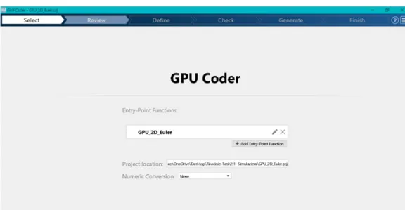
In order to exploit the high computational speed provided by the GPU, the code was translated to CUDA kernels obtained thanks to MATLAB GPU Coder. This useful tool allows to convert MATLAB functions to computationally efficient CUDA code contained inside a MEX file (MATLAB Executable). MEX files are the MATLAB interface to machine code (in this case the GPU-tailored CUDA, which is discussed in section 3.4).

Of course the GPU Coder has many restrictions, namely not every MATLAB built-in function can be translated to CUDA, but its simplicity and the efficiency that can be achieved without knowing another programming language, make it an easy and valuable instrument. Furthermore, any kind of C, C++ or CUDA kernel written by the user can be included inside a MEX file, making up for the lack of built-in functions that can be directly converted.

In order to use the GPU Coder, some preparation steps are necessary:

1. The CUDA toolkit must be installed ([42]). On MATLAB, it is possible to check if this is true by running the gpuDevice command. Other requisites for the use of GPUs on MATLAB, such as the availability of the Parallel computing toolbox, are explained on Mathwork’s site ([43]);

2. It is necessary to add the directive %#codegen, that enables the error check-ing specific to code generation, after the function declaration of every func-tion that is wanted to be converted;

3. To convert the functions to CUDA code, the coder.gpu.kernelfun pragma must be added in the body of the function;

4. Preallocate all the output variables at the beginning of the functions. Steps 2 and 3 can be visualized in Figures 3.1, 3.2 and 3.3, whereas the preal-location step can be appreciated in Figure 3.4.

To sum up, the simulations were obtained by running a script that iteratively calls the Euler’s method function, which in turn iteratively calls the function that I) computes the state variable variations by calling the single cell function and II)

Multiscale analysis of a HCN4 channel double mutation in a human sinoatrial computational model

A

LMA

M

ATER

S

TUDIORUM

· U

NIVERSITÀ DI

B

OLOGNA

S

C

L

M

I

B

(LM)

T

ESI IN

M

ODELLI E

M

ETODI PER LA

C

ARDIOLOGIA

C

OMPUTAZIONALE

LM

Multiscale analysis of an HCN4 channel

double mutation

in a human sinoatrial computational model

Relatore:

STEFANO SEVERI

Correlatori:

FILIPPO CONA

ALAN FABBRI

Candidato:

EUGENIO RICCI

S

ESSIONE

III

A

NNO

A

CCADEMICO

2018/2019

Contents

I

1

II

33

Abstract

Introduction

Chapter 1

The sinoatrial node

1.1

Structure-function relationship of the SAN

1.2

Mathematical modeling of the SAN

1.2.1

Fabbri model

1.3

HCN channels

1.3.1

Structure and physiology

1.3.2

HCN4 mutations

Chapter 2

Elements Read GUI: a User

Interface to display and analyze

electrophysiology experimental data

2.1

Introduction

2.1.1

Aims

2.2

GUI Implementation

2.2.1

ABF format