Corso di Laurea Magistrale in Ingegneria e Scienze Informatiche
Cross-simulator integration:
ns3 as a network simulation back-end
for Alchemist
Relatore:
Prof. Mirko Viroli
Correlatore:
Ing. Danilo Pianini
Presentata da:
Giacomo Scaparrotti
Prima Sessione di Laurea
Anno Accademico 2018/2019
Innovative distributed systems are often studied with the aid of simulation, especially in the case of large scale and situated systems. One of the key aspects of distributed systems is the presence of a set of nodes which must communicate with each other in order to perform their collective task. Consequently, the behaviour of the network plays a key role in determining how the distributed system will act as a whole, but support for realistic simulation of network communication may not be available in simulators that focus on higher-level phenomena, such as the execution of a program on the nodes belonging to a distributed system. Network simulation is usually performed with dedicated simulators which, on the other hand, mostly focus on low-level aspects, such as the behaviour of the physical channels and of the network protocols. The present works aims at filling this gap between high-level distributed system simulation and low-level network simulation by creating a cross-simulator integration between Alchemist, a simulator for large scale situated distributed systems, and ns3, a network simulator, which has been exploited in order to give Alchemist the ability to accurately simulate the network interactions be-tween the nodes. Finally, the whole system has been tested to demonstrate how different network setups can affect the execution of a program in a distributed system.
1 Background 2 1.1 Context and Motivation . . . 2 1.2 Co-simulation approaches . . . 3
2 Domain Analysis 6
2.1 Tools for realistic network simulation: Network Simulator 3 (ns3) . . . . 6 2.2 The Alchemist networking model . . . 11 2.2.1 Networking in the Protelis incarnation . . . 14
3 Architecture 15
3.1 Simplified native interface for ns3: ns3asy . . . 15 3.2 Java bindings for the simplified native interface: ns3asy-bindings . . . 23
4 Cross-simulator integration 31
4.1 Integration of realistic network simulation in Alchemist . . . 31 4.1.1 Integration with the Protelis incarnation . . . 34
5 Evaluation 39
6 Conclusion and future work 46
Bibliography 48
1
Background
1.1
Context and Motivation
Alchemist [1] is a Discrete Event Simulator (DES) [2, 3], which is a kind of simula-tor where the events are executed one at a time moving forward the simulation time consequently [4]. This approach allows to easily model events distributed with various temporal distributions. The typical scenarios can involve many different phenomena, from chemical reactions [5] to pedestrians movement [6, 7].
In Alchemist, the domain entities can be reified in many different ways. To model this aspect, the concept of Incarnation has been introduced, which is a specialization the the Alchemist model that helps to define specific kinds of simulations, allowing for the specification of the concrete implementations of the Alchemist abstract entities should be made, performing a model-to-model translation (M2M).
Among the other things, Alchemist is used to simulate the execution of distributed programs [8]. A distributed system requires the nodes to be able to communicate with each other. The communication can be performed using different technologies, each one having its own peculiarities. For example, if the nodes are connected using a wireless network, their communication will probably experience a higher delay than the one ob-tainable with a wired network. There are also examples of systems in which the node communicate in non-convenctional ways, such as using sound waves in an underwater environment, whose behaviour is determinant for the whole system design [9]. More generally, the relevance of the network is paramount, because it may affect the way the system behaves as a whole [9, 10].
Unfortunately, Alchemist does not provide a way to simulate the behaviour of a real network. This is not necessarily a problem in certain circumstances; for example, the testing of a new distributed algorithm may not need an accurate representation of the network, since that is not the purpose of the simulation. There have also been some cases where a simplified model of a network has been used inside Alchemist [8], but this is clearly not ideal. However, if the behaviour of the network is actually consid-ered a crucial aspect of the system, there is the need to realistically simulate it as well. Modern networks are based on a plethora of technologies and protocols, so it would be very difficult to accurately and reliably model them inside Alchemist. However, there are some specialized simulators whose aim is to provide a convenient and realistic way to simulate a network. Consequently, a sensible approach would be to integrate one of these simulator with Alchemist, exploiting it for the simulation of the communications and using Alchemist to simulate all the other aspects of the distributed system, such as the execution of the program itself.
The integration between Alchemist and a network simulator has been the aim of this work, which led to the creation of a co-simulation system that makes it possible to re-alistically simulate network communication in a simulated distributed system. This has been done by exploiting ns3, a network simulator which supports many different proto-cols and technologies, has high performance and is open source. ns3 has been integrated with Alchemist by creating two libraries: the first one allows for the usage of ns3 as a black box, while the second one makes it possible to use ns3, which is written in C++, from Alchemist, which is written in Java.
To evaluate the capabilities of the co-simulation system, a testbed simulation has been created, involving the exchange of messages in a distributed system using different com-munication technologies. The results demonstrated the effectiveness of the system as a whole.
1.2
Co-simulation approaches
There have been some previous works in which multiple simulators have been used to-gether to manage different aspects of a single task. In many articles, this approach is defined as co-simulation [11]. Most of the works that deal with networking involve the use of a network simulator which is used together with another simulator that deals with
the phenomena of interest. There are different approaches to co-simulation than mainly differ in the way the simulators communicate with each other, which is an aspect that depends on different factors, such as the technologies used by the simulators (i.e. the programming languages they are written in). If two simulators are written with same programming language, the could be integrated using a shared memory aprroach; oth-erwise, it is possible to do so using a foreign function interface or an indirect form of communication, such as sockets or shared files. The overall simulation will be lead by one of the two simulators, which will act as a master, while the other will act as a slave. In fact, most simulators do not provide a means to integrate them with another simula-tor out-of-the-box, so it must be developed by the user. In [12], a network simulasimula-tor is integrated with a traffic simulator in order to simulate a VANET having both a realistic movement of the vehicles and a realistic network interaction. In this case, the network simulator leads the simulation, making the traffic simulator execute one step at a time based on the network interactions between the vehicles. The two simulators communi-cate indirectly with the use of sockets. This approach is based on the assumption that the network communication constantly determines what happens inside the system, and this is a consequence of the aim of the co-simulation, which is to ”better understand the influence of VANET applications on traffic patterns”. Another proposal is the one in [13], in which a network simulator written in C++ is integrated with a power grid simu-lator written in MATLAB. In this case, the main simusimu-lator works indipendently from the network simulator, synchronizing their internal times only if needed (for example, when a communication should occur). Like in the previous case, the communication between the two simulators is realized using sockets.
In [14], the authors integrated a network simulator with a power system simulator. Con-trarily to what happens in the previous works, the simulators do not interact through sockets, but directly: the authors modified the network simulator to expose an inter-face that could be used by the power simulator. These modifications are puposely built around the specific application, so some modeling of the particular system is present in the network simulator, too.
An even looser coupling between different simulators is proposed in [15]. In this case, the simulator communicate by means of a configuration file that is written by the main simulator and read by the network simulator as a configuration for its task. When the network simulator ends its task, it makes the results available to the main simulator, which will retrieve them later.
It is clear that it is possible to realize a co-simulation platform in many different ways, having the simulators communicate with different methods.
It is interesting to note that these works do not simulate generical distributed systems, but rather very specific scenarios, such as the behaviour of vehicles in traffic or the dis-tribution of electrical energy in the power grid.
Alchemist is able to simulate some sorts of distributed systems (for example, the ones running Protelis program) for which it is currently the only available simulator (and will probably be for a long while), so an approach like the ones described before is needed to bring realistic network simulation into these kind of systems.
To the author’s best knowledge, there are no works where ns3 has been used in conjunc-tion with a Java-based simulator.
2
Domain Analysis
2.1
Tools for realistic network simulation: Network
Simulator 3 (ns3)
Figure 2.1: The ns3 logo
The Network Simulator 3 (ns3) [16, 17, 18, 19] is a discrete-event network simulator for Internet systems, targeting primarily research and education.
ns3 has been chosen for this project because it supports a wide variety of protocols and technologies, it has a high level of performance (more on this below) and is free and open source. Moreover, it has been designed for extensibility, which is necessary for this project, and the use of the simulator is not different from the use of any other library (i.e. there is nothing like special syntax or DSLs). Its main competitors lack some of these features. ns2 has a poorer design and is getting old; OMNET++ is harder to extend, because it is not a specialized simulator, but rather a general purpose one, and it is not open source. One of the fundamental goals in the ns-3 design was to provide a high level of realism of the models, so their implementation is as close as possible to the one found in real operating systems, such as Linux and BSD, whose network stacks heavily influenced the ns3 one [20]. Different simulation tools have taken different approaches to modeling, including the use of specific modeling languages, code generation tools, and component-based programming paradigms. While high-level modeling languages and
simulation-specific programming paradigms have certain advantages, simulating actual implementations accurately is not typically one of their strengths. The higher level of ab-straction can cause simulation results to diverge significantly from experimental results, and therefore an emphasis was placed on realism. For example, ns-3 chose C++ as the programming language because it facilitated the inclusion of C-based implementation code (as a side note, this also proved to be also useful to integrate it with Alchemist). The ns-3 architecture is also similar to the one of the Linux operating system, with internal interfaces (network to device driver) and application interfaces (sockets) that map well to how computers are built today. ns-3 is not a completely new simulator, but rather a synthesis of several previous tools, including ns2, which used to be a reference in its field [19]. An emphasis has been put also on ease of debugging, better alignment with current languages, and performance (the latter being an important aspect for this project) This led the ns3 team away from the mixture of OTcl and C++ found in ns2, which was hard to debug and had less than ideal performance. Instead, the designers chose to put an emphasis on C++-based models for performance and ease of debugging. Figure 2.2 briefly illustrates how ns3 is built:
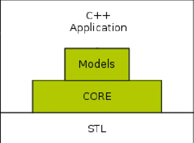
Figure 2.2: Graphical representation of the ns3 architecture. The entire software is based on the C++ Standard Template Library. The Core module provides the basic facilities used by all the Models. The simulation is a C++ application that has access to all of these functionalities.
The main feature of this architecture stands in the fact that simulation are C++ programs theselves, instead of being written in some sort of scripting language (as OTcl for ns2) or in a configuration file. This is not necessarily an advantage for the simulation
itself, but the fact that the simulator’s interface is made to be easily accessible from the outside proved to be useful to integrate it with Alchemist. This also implies that a simulation for ns3 has access both to all its functionalities and to external ones: aside from being dependent from ns3, it is a fully fledged C++ program.
ns3 organizes its functionalities into so-called modules. A module is a part of the simulator which handles a specific aspect of it. These are the most prominent modules: Core This module contains all the basic facilities used by all the other modules. These facilities include smart pointers, callback handlers, attributes manager, logging utilities and random variables.
Network This module contains the models of all the basic components of a network. it is worth citing some of these:
Node A node is communication endpoint. An example of node is a computer in a LAN.
NetDevice A NetDevice is the means used by a node to interact with the network, like a Ethernet adapter inside a computer. The network module also contains a model of the corresponding MAC address.
Socket A socket, just like in operating systems, is a software abstraction which enables an application to communicate across the network.
Application An Application is the equivalent of a program running on a com-puter. An Application runs on a specific Node. It can use sockets to commu-nicate with other Application running on other Nodes. ns3 contains various pre-defined Application (such as an Application which periodically sends a UDP packet) in a ad-hoc module.
Internet The Internet module contains the model for all the protocol normally used on the Internet, such as IPv4, IPv6, ICMP, TCP (with its various version), UDP, etc. Devices modules There are many modules which model various kind of devices, such
as CSMA devices or Wi-Fi devices.
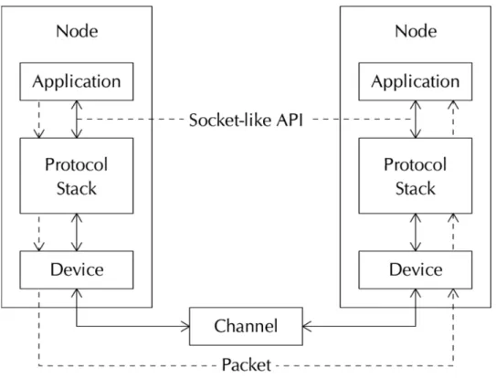
Figure 2.3: Graphical representation of the ns3 network stack
It very closely resembles the actual architecture of a computer network; in fact, even programming an application inside ns3 is very much like programming in a real environment. This eases the development of a simulation.
One of the strengths of ns3 is its accurate reproduction of real devices and protocol along with its performance. In fact, ns3 is one of the fastest network simulators currently available, as shown in Figure 2.4 and 2.5 from [21], where the same simulation, consisting in a number of nodes connected to a wireless network and broadcasting messages, is run on multiple network simulators.
Figure 2.4: This diagram shows how the network size affects the execution time of a reference simulation, which consists in a number of nodes connected to a wireless network and broadcast-ing messages.
Figure 2.5: This diagram shows how the memory occupied by the simulator changes with the size of the network of a reference simulation, which consists in a number of nodes connected to a wireless network and broadcasting messages.
The authors in [21] conclude that “ns-3 is capable of carrying out large-scale network simulations in an efficient way” and that “ns-3 demonstrated the best overall perfor-mance”, making it a good choice for its integration with Alchemist, taking into account its application in simulating large scale distributed systems.
2.2
The Alchemist networking model
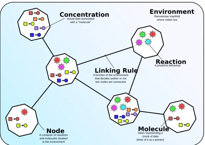
Alchemist [1] is a Discrete Event Simulator (DES) [2, 3] based on the Next Reaction Method from Gibson and Bruck [22], featuring a chemistry inspired meta-model. As a consequence of this aspect, the terminology used for the various simulated entities resembles the one commonly used in chemistry. These are the main concepts:
Node A Node is an entity situated in the Environment. A Node is a sort of container in which there are other entities, called Molecules, which have an associated Con-centration.
Reaction A Reaction is an event that can change the state of the Environment. Every Node have a (possibily empty) set of Reactions. Each Reaction is in turn made up by a set of Actions. A Reaction is triggered by a certain Time Distribution, which determines when a Reaction should happen, and only if a set of Conditions is satisfied.
Neighborhood The Neighborhood is a set of Nodes connected to a central Node. Every Node has its (possibly empty) Neighborhood.
Linking Rule The Linking Rule is the criterion used to determine which Nodes belong to a certain other Node’s Neighborhood.
Figure 2.6: The main entities of the Alchemist model. When two or more nodes are connected according to a certain Linking Rule, they must be able to communicate with each other.
Alchemist does not impose a fixed interpretation of Molecule and Concentration, whose definition is demanded to specific Incarnations.
In the context of networking, the main entities of interest are the Neighborhood and the Linking Rule. If a Node is intended as a node in a network, the Nodes in a certain Neighborhood, which is determined by the given Linking Rule, should be able to com-municate with each other. Since the Alchemist meta-model is deliberately generic, it doesn’t define how different Node should communicate, because the concept of commu-nication can have different meanings in different settings. This means that this should be determined by each Incarnation.
At the moment, no incarnation provides a means to handle realistic network commu-nication, even the ones specifically aimed at distributed computing, such as the Protelis
incarnation.
2.2.1
Networking in the Protelis incarnation
Protelis[23] is a programming language based on Field Calculus[24] and inspired from the Proto language [25], which has been puposedly made for writing programs that should be executed on aggregates of devices. A system of devices running a Protelis program is, in fact, a distributed system.
Protelis is an interpreted language whose virtual machine is written in Java. The execu-tion of a Protelis program involves the presence of a so-called Execuexecu-tion Context, which is an interface between the Protelis program and the environment the devices is located in. When a Protelis program is run inside Alchemist, the Execution Context is provided by Alchemist itself, making it a fundamental part of the system.
Since the nodes that run a Protelis program are distributed in the environment, the way they interact through the network plays a fundamental role. Despite this, the Protelis incarnation does not provide a means to realistically simulate these interaction. Some attempts have been made in the past to mitigate this issue: an example can be found in [8], where a delay has been added to the messages’ reception in order to emulate the network’s real behaviour, according to a formula like the following one:
d = p + s b
where d is the delay, p is the propagation delay, s is the packet size and b is the data rate. This is different from what really happens in a network, where, for instance, the delays are not fixed and a message is potentially divided in more parts on the physical level, each one handled individually. This method can assess a base level of perfor-mance for the distributed system by introducing a pessimistic delay, but it fails when the aim is to determine the real requirements to deploy the system in a real setting and, more generically, to understand how the system performs with a certain level of precision. Anyway, the complexity of a networks spreads far beyond a simple matter of delays, and this approach, albeit easy to implement, can capture only a small part of it. A novel approach is needed: this will be the subject of the next chapters.
3
Architecture
3.1
Simplified native interface for ns3: ns3asy
As discussed in the previous chapter, ns3 is a very rich simulator, but it is also a rather complex piece of software, which means that even setting up the most basic simulation requires writing a lot of code: a network between two nodes can be made by a number of different technologies, both at the physical and at the logical (protocols) level, and each one must be configured individually. Anyway, most networks only use a limited subset of all the possible technologies: in a home and office context, most nodes will be prob-ably connected using Ethernet or 802.11 Wi-Fi at the physical and link levels, and will probably use IP at the network level and TCP or UDP at the transport level; also, since the vast majority of the nodes uses some kind of operating system, the communication will be mediated by a socket.
Having this more restricted framework to deal with, ns3asy has been created, which is a new ns3 module whose aim is to provide access to many common network function-alities in a simple way. Its architecture is somewhat similar to the one in [14], but with a more generic approach: ns3 is not made aware of the nature of the whole simulation; it only has to deal with the networking aspect. The interface provided by ns3asy is simple: first of all, the user must define the network topology (how the nodes are connected to each other), then zie must choose which physical technology (currently, Ethernet and Wi-Fi are supported) and which transport protocol (TCP or UDP) to use. For each technology, it is optionally possible to specify some other parameters (for example, in the case of Ethernet, it is possible to specify the channel’s error rate). Finally, zie can
register a function as a callback which will be called when a node receives a packet (call-backs can be resitered also to receive notification upon packet sending and, if TCP is used, connection creation and deletion). ns3asy already provides its default callbacks, which print on the standard output the current operation and the packet’s content. After these operations, which can be done with a small number of lines of code, the user can start to send packets, whose transmission will be simulated by ns3.
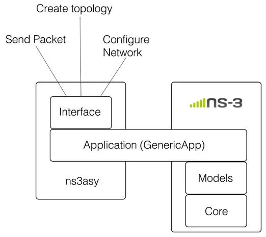
Figure 3.1 illustrates how ns3asy works compared to the barebone ns3:
Figure 3.1: Graphical representation of how ns3asy integrates with ns3 (please refer also the to Figure 2.3 in the previous chapter). The main difference stands in the application level: instead of having a ad-hoc application for each simulation, ns3asy gives the user the ability to access ns3’s feature using a simple interfaces that allows for sending and receiving packets through the simulated network. The inner workings of ns3 are consequently transparent to the user.
As illustrated, each node runs an Application called GenericApp, which acts as a bridge between ns3 and the user. GenericApp exposes an API which allows to user to send and receive data through it, without having to deal directly with ns3. From the Application’s standpoint, what happens inside ns3 is not a concern: GenericApp makes ns3 transparent with regards to the user, allowing him to use the network through a socket-like interface. This is actually close to what happens when running a ’normal’ application which relies on the operating system to deal with the network: the
applica-tion only has to deal with sockets, but it doesn’t have to care about the inner workings of the network.
The diagram in Figure 3.2 shows how ns3asy is structured:
Figure 3.2: Diagram which illustrates how ns3asy is structured. ns3asy provides an interface built on top of a ns3 Application, allowing for sending packets and configuring the network without having to deal directly with ns3.
The example in Listing 3.1 illustrates how to set up a simple simulation using ns3asy: Listing 3.1: Example of usage of ns3asy to create a simple simulation.
1 //there are two nodes in the simulation
2 SetNodesCount(2);
3 //the first node is connected to the second node (but not the other way round)
4 AddLink(0, 1);
5 /*
6 * Ethernet will be used, with TCP (’false’ in the first parameter), default packet
7 * size, 0.0001 as the error rate of the physical channel, and a data rate of 1 Mbps
8 */
9 FinalizeSimulationSetup(false, 0, 0.0001, "1Mbps"); 10 //10 packets will be sent
11 for (unsigned int i = 0; i < 10; i++) {
12 /*
13 * The packet will be sent by the node with id ’0’, a single copy of the
14 * packet will be sent with this function call, the content of the
15 * packet will be "test", which is an array of char with size 4
16 */
17 SchedulePacketsSending(0, 1, "test", 4);
18 }
19 //Actually send the packets
20 ResumeSimulation(-1);
21 //Close the connection and terminate the simulation
22 StopSimulation();
The SchedulePacketSending function makes a socket inside GenericApp send a packet containing the provided payload, which will be received by the recipient trig-gering its receive callback. A set of built-in callbacks is provided with ns3asy, which make GenericApp print what’s happening inside it (these are the callbacks used in the previous example). Clearly, when used in a ”real” context, the user will provide his own callbacks that will handle the events according to the aim of the considered simulation (for example, instead of simply writing the received packets on the standard output, the user might want to store them in order to evaluate them).
At the moment, ns3asy supports the following technologies: Physical level and Data Link level
– CSMA (An Ethernet-like technology, which shares the same carrier sense mul-tiple access logic, albeit in a simplified way)
– Wi-Fi (With support for node and access point positioning and for all the propagation models provided by ns3)
Network level – IPv4 Transport level
– TCP (With the New Reno congestion control algorithm [26]) – UDP
Application level
– Any program that can interact with ns3asy with the corresponding C interface When refering to specific physical technologies, it is possible to configure other specific parameters:
CSMA
Data rate The maximum data rate supported by the physical medium, e.g. 100 Mbps. By default, the channel provides a gigabit grade data rate, but it is possible to specify any data rate.
Error Rate The error rate is used to determine if a byte in a certain frame will get corrupted.This done by applying the following formula:
c ← r < [1 − (1 − e)s]
where c is a boolean variable which determines is a packet will get corrupted or not, e is the provided error rate, s is the packet size (at the physical level) and r is a random variable. By default, r is determined by a uniform distri-bution which uses the same seed at each simulation run, in order to obtain
a deterministic behaviour of the simulation. Because s is at the exponent on the right hand side of the equation, the probability of losing a packet is pro-portional to its size; in other words, a large packet has a greater probability of being lost than a small one (in the same circumstance). As a consequence, the provided error rate does not immediately determine how many packets will be lost, because it also depends on how large they are. ns3 allows to use different error models but, at the moment, this is the only one supported by ns3asy for CSMA. Anyway, it is also one of the closest to real life networks, as many other ones are a further simplification of this algorithm.
Wi-Fi
Access point position It is possible to set a position for the access point. Nodes positions It is possible to set a position for each node. This is mandatory. Propagation delay model The propagation delay model is used to determine the time taken from the Wi-Fi radio signal to go from the source to the destination. There is no default propagation delay model; however, the model used in most simulations has been the Constant Speed Propagation Model, which assumes the signal to always propagate with the same speed c (the speed of light). ns3 provides only another propagation delay model, which determines the delay starting from a random distribution.
Propagation loss model The propagation loss model is used to determine how the radio signal gets attenuated as it travels through space. There is no default propagation delay model; however, the model used in most simulations has been the Logarithmic Distance Propagation Loss Model, which determines the path loss L according to the following formula:
L = L0+ 10n log10
d d0
where L is the path loss, L0 is the path loss at reference distance, d is the
distance between the transmitter and the receiver, d0 is the reference distance
(by default, it is 1 meter) and n is the path loss exponent. By default, the path loss exponent n is 3, which is empirically considered a value which accounts for the average loss in different environments: in free space, a good value for n is 2, while indoor a good value is 4. Being merely an exponent, n does not
have a unit of measurement. Despite being relatively simple, this model is actually capable of representing the path loss with a good level of accuracy [27]. This model has been considered a good compromise between simplicity and accuracy, at least for the experiments that have been done to demonstrate the functionality of ns3asy (more details in the following chapters). Anyway, every model available in ns3 is also available in ns3asy. There are models which simulate the behaviour of Wi-Fi signals in different scenarios, such as in buildings, outdoors, NLoS (non line of sight), etc...
It must be noted that GenericApp, which constitutes the main link between ns3 and an outer program, is not strictly tied to any of these technologies (for example, the creation of the sockets used by each GenericApp doesn’t happen inside the GenericApp class itself, so any kind of socket based on any technology can be used); this means that ns3asy’s functionalities can be expanded mostly without modifying what already exists, but rather only adding new pieces of code.
It is clear that creating a simulation using ns3asy hides many technicalities which may not be necessary in certain contexts: if, for example, the aim of the simulation is to determine how long a certain amount of packets takes to be trasmitted from one node to another, ns3asy is perfectly suited.
In order to achieve this level of simplicity, it has been necessary to simplify some aspects of the configuration. The following aspects are the most remarkable ones: All the nodes share the same communication technology It is not possible to
de-fine a network in which different nodes are connected using different communication technologies (i.e. some with Ethernet and some with Wi-Fi). This may sound lim-iting, but it can be a perfectly reasonable trade-off: simplicity has been considered one of the key goals during the design of ns3asy, so configurability had a lower priority.
All the nodes share the same physical link Again, this is due to the will to keep ns3asy as simple as possible. It must be noted that, in fact, this is not as limiting as it may sound: ns3 makes some simplification regarding the simulation of the physical layer which make this feature less relevant. For example, Ethernet imple-mentation does not simulate collisions on the physical medium; instead, a busy flag
is used to signal whether the channel can be used or not. This means that there are no retransmission due to collisions, thus relieving the trafic on the channel and making it less influenced by the number of connected node.
It is not possible to run multiple instances of ns3 from the same process This is a limitation derived from the design of ns3 itself, which is inherently single-threaded. Anyway, it must be noted that there isn’t a standardized way of manag-ing thread from whithin a C program and, until recently, it did not exist in C++, neither. Actually, Alchemist also uses a single thread when executing a single simu-lation, leveraging multithreading only when there are multiple batched simulations in queue. When using ns3asy as a stand-alone product, this is not that much of an issue, because it just replicates the same limitation that’s present in ns3. The nodes cannot move Albeit ns3 provides a mobility model which allows the nodes
the move inside an environment, this functionality is not available through ns3asy. This is clearly not a concern when it comes to wired networking, but it can be a limit with wireless links. However, it is possible to assign a certain position to each node before the simulation start, which, for the moment, has been considered a viable trade-off.
These aspects are partially a consequence of the necessity to provide a pure C interface to ns3asy, thus making it impossible to expose it using the object-oriented abstractions provided by C++. This makes it necessary to wrap every functionality exposed by ns3 in an object oriented way into a vanilla C function, which requires an additional effort. The reason for this necessity has to do with how the integration with the Java platform works (this aspect will be covered in the next section). A side effect of this stands in the necessity of managing the memory with the functions provided by the C Standard Library, such as malloc. These functions are considered as legacy when used in C++ [28], but they are necessary, for example, in order for a function to safely return a string as an array of char. Since fully manual memory management tends to be very error prone, proper tools have been used in order to minimize the chance of having such errors, the main one being Valgrind Memcheck [29], which helped preventing some subtle error entering mainline.
3.2
Java bindings for the simplified native interface:
ns3asy-bindings
One big downside of ns3asy is its native nature: ns3asy, just like ns3, is written in C++ (actually, this is necessary in order to be able to access ns3’s functionalities) and exposes its interface as a C library, so a simulation which makes use of it must be written in C or C++, too. Even without thinking about the main reason why this project took place (being able to use ns3 from Alchemist), this is bothersome: C and C++ are languages that are rather difficult to use, especially for an inexperienced programmer, and this can be a deterrent for those who would like to use ns3’s functionalities but don’t have the ability to do so.
In order to provide the ability to use ns3asy with an higher-level language, ns3asy-bindings has been created. ns3asy-ns3asy-bindings provides the ability to use ns3asy from a program written in any JVM-compatible language, and is itself written in Java. To the author’s best knowledge, this is the only library which allows the usage of ns3 with a language different from C++ (actually, ns3 comes with some automatically generated bindings for Python, but they are just mere wrappers for the C++ interfaces, and share the same conceptual level of complexity, along with the fact that they’re very scarcely documented).
This result has been achieved leveraging Java Native Access (JNA), which is a library that allows a Java program to invoke a native library just by defining its interface and its location. This is different from what Java Native Interface (JNI) does, because JNI requires the native library to aware of java’s existence: in JNI, two pointers, one to the Java environment and one to the calling object, are always provided as parameters to the native functions, which must be defined consequenly. Also, the header files are usually generated starting from the Java code using javac. On the contrary, JNA allows the programmer to write the native code as usual, without the need to care about what happens inside the JVM. In order to achieve this, JNA leverages a native library call libffi (where ffi stands for Foreign Function Interface) which deals with all the technicalities such as finding a function inside a compiled library starting from the function’s name and determining its call conventions. This library is what makes possible to find a native function starting only from its name defined inside a Java inteface. To better understand
how JNA works, here is a brief example:
Listing 3.2: Example of usage of JNA to map a function called printf located in the c library to a Java method
1 import com.sun.jna.Library; 2
3 public interface MyNativeLibrary extends Library {
4 MyNativeLibrary INSTANCE = (MyNativeLibrary) Native.
loadLibrary("c", MyNativeLibrary.class);
5 void printf(String format, Object... args);
6 }
This piece of code allows the use of a function called printf which can be found inside a library called c. There is also a static object inside the interfaces which serves as a way to access it.
It is worth taking a closer look at how this actually works, and why. When the loadLibrary static method of the Native class is called (line 4), JNA will look inside the native li-brary called c searching for a function named printf that can accept a String and an array of Object as parameters. JNA ’knows’ different ways to convert a Java object, such as String, into a valid C data type (for example, a String can be converted into a char*), and, unless the user wants to specify a special way to do so, the built-in methods are fine. If JNA manages to find all the declared methods in the native library (in this case, it is only necessary to find the printf function), an object that adheres to the provided inteface is created and put inside the INSTANCE static field.
The native library can consequently be used this way:
Listing 3.3: Usage of the library loaded with the code shown in Listing 3.2 1 import JNAApiInterface;
2 import com.sun.jna.Native; 3
4 public class Example {
5 public static void main(String args[]) {
6 MyNativeLibrary lib = MyNativeLibrary.INSTANCE;
7 lib.printf("Hello World");
8 }
This is all that’s needed to use JNA, meaning that the native library does not need to be modified in any way. From this point of view, JNA has a big advantage over JNI. The main downside of JNA, at least for what concerns this project, is its inability to call functions written in C++: only vanilla C is supported. In fact, a compiled C++ program differs from a C one, among the other things, in virtual table layout, exception handling, the structure of its stack frames, because it has to deal not only with plain data, but also with objects, and in the fact that function names are consequently man-gled, even for purely procedural ones. This limitation is the reason why the functions defined in ns3asy are actually exported as C functions. The implications of this aspect will be discussed later.
On the one hand, ns3asy-bindings allows the functions defined in ns3asy to be used from Java, but there’s more. Java is not only a programming language, but also a platform with its idioms and its customs. In Java, data input and output is usually performed using a stream, which is an abstraction over what actually happens ”un-der the hood” On the lower level there are the streams for interacting with the actual I/O devices, such as files or serial ports. A ”low-level” stream is only able to read or write individual bytes, but it is possible to wrap it inside a higher-level stream which takes care of transforming something complex in a series of bytes. With the combina-tion of multiple streams it’s possible, for example, to write an entire object to a file and read it back. To comply with this pre-existing idiom, ns3asy-bindings provides its own implementation of the OutputStream and InputStream interfaces: writing to Ns3OutputStream means using the ns3 simulator to send some data from a certain node to another (Ns3InputStream does the inverse operation). The most important aspect is the transparency of this process: the user does not need to know how ns3 works; instead, the only requirement is a basic knowledge of Java’s idioms.
Figure 3.3: Diagram which illustrates how ns3asy-bindings is structured. ns3asy-bindings com-municates with ns3 by means of ns3, which acts as a bridge. It allows to do all the operations allowed by ns3asy, and it also provides a means to integrate with Java streams, that can be used in order to have a smoother integration with the Java platform. A more detailed view is given in the Class Diagram in Figure 3.4.
labelns3asy-bindings
It must be noted that having a simple interface to ns3 is not only a matter of ease of use: when building complex pieces of software, it is necessary to hide the technicalities behind an inteface that exposes to the user only what really matters to him, and this is exactly what ns3asy-bindings does. In other words, if the user had to deal directly with the underlying ns3asy interface, the code which made use of it would be bloated with implementation details which would jeopardize its development.
Listing 3.4: Example of usage of ns3asy-bindings. The signature of the methods loaded from the native library are the same as in Listing 3.1. The main feature of this example is the usage of the Streams provided by ns3asy-bindings to send and receive data through ns3
1 public void example() throws IOException, ClassNotFoundException {
2 final int nodesCount = 2;
3 final NS3Gateway gateway = new NS3Gateway();
4 NS3asy.INSTANCE.setNodesCount(nodesCount); 5 NS3asy.INSTANCE.addLink(0, 1); 6 7 NS3asy.INSTANCE.finalizeSimulationSetup(false, 0, 0.002, "1 Mbps"); 8
9 final Object toSendObject = new Date(); 10
11 final NS3OutputStream ns3OutputStream = new NS3OutputStream(
gateway, 0, false);
12 final ObjectOutputStream oos = new ObjectOutputStream( ns3OutputStream);
13 oos.writeObject(toSendObject);
14 oos.close();
15
16 final Endpoint receiver = gateway.getReceivers().get(0); 17 final Endpoint sender = gateway.getSenders(receiver).get(0); 18
19 //flawless integration with Java idioms
20 final NS3asyInputStream ns3asyInputStream = new
NS3asyInputStream(gateway, sender, receiver); 21 final ObjectInputStream ois = new ObjectInputStream(
ns3asyInputStream);
22 final Object receivedObject = ois.readObject();
23 ois.close();
24
26 }
In this example, a Date object is created (it could be any other Java object), sent through ns3 from one node to the other, read back and printed on screen. It must be noted that the object actually passed through a whole simulated network (it wasn’t just copied). In other words, toSendObject and receivedObject are equals accord-ing to their equals method, but they’re not the same object (toSendObject == receivedObjectis false).
The NS3Gateway class deserves a closer look. In ns3, the arrival of a packet is per-formed by calling a callback bound to the receiving node, which accepts as a parameter the whole packet. This is an idiom of the simulator, and therefore cannot be changed, but, in Java, an InputStream reads the bytes one at a time. The NS3Gateway class aims at filling this gap: when a NS3Gateway object is created, it registers itself as the callback, so it can store the received packets into an internal data structure. When the InputStream is created, it is given the NS3Gateway object as a parameter, from which it can read the received bytes one at a time, as it should.
ns3asy-bindings allows for the setting of all the configurations listed for ns3asy, thus enabling the use of all the technologies listed in the previous section.
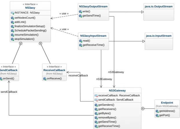
Figure 3.4: UML Class Diagram which illustrates how ns3asy is structured. The NS3asy in-terface, which can be used through its INSTANCE static field, provides the means to interact with the underlying ns3 simulator, including the ones used to configure the network, to send a packet, and to actually execute the simulation. The Streams make use of the NS3asy ob-ject, to directly interact with the ns3 simulator, and of the Ns3Gateway obob-ject, which is used, as described before, as a receiver for the callbacks coming from ns3. The diagram is slightly simplified with respect to the real implementation for clarity’s sake.
It is interesting to note that the signatures of the methods closely resemble the one of the corresponding C functions. In fact, JNA is able to perform the necessary conversions when needed (for example, it can convert a String object into an array of char), but at the same time it does so only when strictly needed (for example, it may not be necessary to convert a Java native array, such as int[], into the corresponding C one, because it would be passed by reference anyway), leading to good performance in most
4
Cross-simulator integration
4.1
Integration of realistic network simulation in
Al-chemist
The main reason why the previous libraries have been developed has been their integra-tion in the Alchemist simulator. As stated previously, the lack of a realistic representaintegra-tion of network communication can be an issue for some of Alchemist’s application, especially the ones in the field of distributed computing, so there was to need to provide a concrete answer.
Given its general purpose nature, Alchemist does not impose a pre-defined network model, as different incarnations may want to handle this aspect differently. The only requisite is for the nodes belonging to a certain Neighborhood to be able to communicate with each other. Generally speaking, the integration between Alchemist and ns3 would work as follows:
1. A node requires Alchemist to send a message to a neighbor 2. Alchemist passes the request to ns3
3. ns3 simulates the process of sending the message
4. When done, ns3 tells Alchemist if the message arrived and how much time t it took 5. Alchemist schedules a new event at time t consisting in the arrival of the message
6. The neighbor receives the message at time t
Clearly, the previous process exploits ns3asy and ns3asy-bindings to make Alchemist and ns3 cooperate. It is interesting to note that there is no explicit synchonization of the simulation times between Alchemist and ns3; in fact, this is not a mandatory feature: what really matters are the time intervals, and not its absolute value. In other words, it is not relevant to know the exact moments when a message is sent and received, but rather the time interval between its departure and its arrival. As a consequence, the internal times of Alchemist and ns3 may drift apart, but this does not affect the overall simulation. As a consequence of this approach, when the network simulator is running, it is not possible to add further events until it stops. Moreover, ns3 is involved in the simulation only when a communication act happens (third point of the previous list); in every other moment, it is not running. Alchemist is the simulator which leads the overall simulation, therefore it is the master. It can be said that the coupling between Alchemist and ns3 is loose, where having a tight coupling would mean to costantly maintain the time synchronization between the two simulators. A loose integration is certainly simpler than a strict one, because each simulator can run almost indipendently from the other, exchanging data with it only when really needed.
If there is the need to send a Java object through a network, be it a real or a sim-ulated one, it necessary to serialize it. Java provides a built-in facility so serialize and deserialize objects, but it has been subject to criticism, mainly because of its poor per-formance due to the will of its designers to make it possible to recreate an entire object graph, even though the vast majority of use cases for serialization don’t involve serializ-ing programs, but merely serializserializ-ing data. The integration of ns3asy with Alchemist has been built with this aspect in mind, allowing the user to adopt any serialization frame-work of its choice. The built-in implementation makes use of Java’s serialization facilities. Since Alchemist’s functions are divided into so-called modules, an ad-hoc module has been created for the integration with ns3, called ”alchemist-ns3”. This module provides access to the functions provided by ns3asy through ns3asy-bindings and to the serializa-tion facilities. A class called AlchemistNs3, along with a so-called Serializer, act as a bridge between Alchemist and ns3asy-bindings. The module’s behaviour (e.g. the technology that must be used at the physical layer) can be configured through a YAML file, just like every other aspect of the simulation.
The diagram in Figure 4.1 shows how the alchemist-ns3 module works in conjunction with ns3:
Figure 4.1: Diagram which illustrates how the alchemist-ns3 module works in conjunction with ns3. The network is configured according to the provided YAML file. When a node belonging to a certain incarnation needs to send a message, it sends its request to alchemist-ns3, which delegates the operation to ns3asy-bindings, according to the mechanism discussed in the previous chapter. When a message is received inside ns3, alchemist-ns3 delivers it to the corresponding node inside Alchemist. In the next section, a more thorough explaination is given refering to a specific incarnation.
In Listing 4.1 there is an example of a configuration for alchemist-ns3. Listing 4.1: Configuration for Alchemist of a CSMA network
1 [...]
2
3 ns3:
4 protocol: "TCP"
6 error-rate: 0.0001 7 data-rate: "1Mbps" 8 serializer: 9 type: it.unibo.alchemist.ns3.utils.DefaultNs3Serializer 10 11 [...]
In this example, a CSMA network is created with the provided packet size, data rate, error rate, and serializer. The number of nodes and their positions are determined from their displacements.
The concept of communication can have different meanings in different incarnations. It can be said that having a realistic network simulation in Alchemist only makes sense when dealing with distributed systems. One of the incarnations dealing with distributed systems is the Protelis incarnation, so this has been considered the most natural choice for developing a concrete implementation of realistic network simulation.
4.1.1
Integration with the Protelis incarnation
In a distributed system, communication between nodes is of paramount importance. The system can tackle its task only if its components are able to cooperate, and they do so by exchanging information using some sort of network; systems running Protelis programs are no exception. Protelis is different from other languages in the fact that it has been made to define the behaviour of a system in its entirety, but when it comes to what each node do, there is still the need to make it communicate over a network. As described in a previous chapter, Alchemist did not provide any way to actually simulate a network in a realistic manner, but the way it handled network communication was prone to this sort of addition.
Before describing how ns3 has been integrated in the Protelis incarnation, let’s have a look at how networking for Protelis is handled in Alchemist from a generic perspec-tive. A Protelis program runs inside its own virtual machine, which in turn runs on the JVM. When a Protelis program, running in its own Protelis virtual machine, needs to send a message to another node (for this explaination, it doesn’t matter what’s in-side these messages), it does so by calling a specific function provided by the
Execu-tion Context, which is an interface between a Protelis virtual machine and environ-ment in which it is executing. When a Protelis program is run inside Alchemist, the Execution Context is provided by Alchemist itself, in the form of a dedicated class, called AlchemistExecutionContext, containing all the necessary functions, in-cluding the one, called shareState(), used by the nodes to send a message. When shareState() is called by the Protelis virtual machine, it delegates the actual mes-sage sending to a so-called network manager, which is implemented by the
AlchemistNetworkManager class. This class must take the message and deliver it to the corresponding recipient.
In its basic form, this is done by simply sharing the object containing the message with the recipient. In the implementation bundled with Alchemist, this operation is completed istantaneously, so their is basically no realism about the networking aspect. Memory sharing is clearly good from a performance perspective, as not having to allo-cate more memory makes the program save time, but this is clearly different from what happens in a real network, whose implementation cannot be based upon this method.
This is where ns3 comes into play. Instead of sharing the message between the sender and the recipient, a realistic network simulation is carried out by having the latter re-ceive the message after is has been delivered through the network simulated by ns3. As pointed out in a previous chapter, this is done by actually simulating the inner workings of all the devices which would be involed if a real network was used, and the delivered message is not merely the sent one, but is an actual brand new message recreated at the other end of the network.
The pseudo-code in Algorithm 1 wraps up the process.
When the executing Protelis program needs to send a message to a Neighbor, the vir-tual machine it is running on delegates the operation to Alchemist, which is the hosting platform. In turn, Alchemist, after having serialized the message, passes it to ns3 through ns3asy. ns3 realistically simulates the message delivery and, when it’s done, makes the message received by the recipient available to Alchemist, along with two timestamps: one for the time at which the message was sent, and one for the time at which the mes-sage was received. As stated before, their absolute values might differ from Alchemist’s
Algorithm 1 Realistic message delivery
1: procedure SimulateRealisticMessageArrival 2: begin procedure
3: msg ← message to be delivered 4: toSend ← serialize(msg) 5: for each neighbor :
6: send(toSend) //sends a message through ns3
7: rcvd ← deserialize(receive()) //receives that message through ns3 8: sendTime ← time at which the message was sent
9: recTime ← time at which the message was received 10: delta ← recTime - sendTime
11: scheduleEvent(rcvd, delta) 12: end procedure
internal time, but what really matter is instead the resulting delta (their difference). The delta is used to determine the moment at which the message should actually be received by the recipient inside Alchemist. To make the recipient actually receive the message, a corresponding event is scheduled inside Alchemist. When the moment comes, the recip-ient will receive its message. If, for some reason, the message gets lost (for example, due to an error on the physical medium), no event will be scheduled. An event is actually a Reaction, whose only corresponding Action consists in the message receival.
This entire process is implemented inside the AlchemistNetworkManager class, which makes use of the AlchemistNs3 class described in the previous section.
In order to support this flow, Alchemist’s engine has been modified to support runtime Reaction add and removal, an operation which was previously not possible. This is clearly necessary in order to add an event at runtime to an already existing Node.
The UML Class Diagram in Figure 4.2 shows how ns3asy is used inside the Protelis incarnation:
Figure 4.2: UML Class Diagram which illustrates how ns3asy is integrated inside the Protelis incarnation. AlchemistNetworkManager, whose objects are used by each Protelis node to com-municate with the others, uses NS3asyOutputStream and Ns3asyInputStream to simulate the arrival of the messages to the neighbors and evaluate the time each message took to arrive. The Ns3Gateway object used to handle the received data and the Serializer object are statically provided by the AlchemistNs3 class, which is configured when the simulation is loaded.
Figure 4.3: UML Sequence Diagram which illustrates how the Protelis incarnation makes use of ns3 through ns3asy in order to achieve realistic network simulation. The lifelines with a yellow background represent entities living inside the Java Virtual Machine, while the ones with a blue background represent entities written in C and C++, and consequently living in a native environment. The represented entities do not fully reflect the real ones for simplicity’s sake. The diagram refers to a single neighbor: the entire procedure shall be repeated for each neighbor.
This diagram also makes it clear how JNA is used to integrate ns3 inside Alchemist through ns3asy and ns3asy-bindings. It might be interesting to evaluate how much JNA impacts on the overall performance of Alchemist; this topic will be covered in the next chapter.
5
Evaluation
In order to evaluate how a real network affects the performance of a simulation that makes use of it, a testbed simulation has been realized. Since the integration of ns3 with Alchemist has been implemented only for the Protelis incarnation, this is the one that has been used. This reflects one of the main reasons why ns3 has been integrated with Alchemist in the first place: having a realistic network simulation for distributed applications, for which Protelis has been purposely made.
The testbed application tackles the following task: a certain number of node is laid out in the environment; one node is labeled as ”source”, while another one is labeled as ”destination”. The aim of the program is to create a gradient going from the source to the destination, based on the distance between each node. The environment has two dimensions, so the distance between the nodes is an euclidean one.
The gradient is evaluated by a program written in Protelis, which is then executed by the corresponding virtual machine hosted by Alchemist. In order to calculate the dis-tances between the nodes, each node has to communicate with its neighbors: a node can calculate its distance from a neighbor, but not from the nodes outside its neighborhood. This is where the integration between ns3 and Alchemist comes into play.
The experiment consists in the execution of such program with different network con-figurations. Both CSMA and Wi-Fi have been used, in order to have a full coverage of the implemented features. In all cases, the program is run until the Alchemist environ-ment is stable, which is, until there are no further changes in the nodes it contains, for a certain number of simulation steps. The simulation is considered finished when this
condition is met. At that point, the environment should be like in Figure 5.1.
Figure 5.1: Representation of how the environment should be at the end of the test simulation. Each node has a different hue depending on its distance from the source node, which is located on the bottom left (the one with a yellow dot). On the side of each node there is the indication of its distance from the source.
The first experiment involves the use of a CSMA (Ethernet like) network. At each run, the channel error rate has been changed in order to evaluate its impact on the time needed to spread the information about the gradient. As a reminder, this is the formula used to map the provided value into an actual error rate:
where c is a boolean variable which determines is a packet will get corrupted or not, e is the provided error rate, s is the packet size (at the physical level) and r is a random variable. When evaluating the results, it must be noted that, using this formula, the probability of losing a packet is proportional to its size. By default, a CSMA channel has a MTU of 1500 bytes (just like Ethernet), but the upper protocols (like TCP) do not necessarily use the entire MTU, so a certain error rate value does not immediately map to a certain error rate on the physical channel. This may seem counterintuitive, but it actually lead to a behaviour which is close to what actually happens in real networks: small packets have a smaller chance of getting corrupted than larger ones.
The network has been configured with the following parameters:
1 [...]
2
3 ns3:
4 protocol: "TCP"
5 error-rate: [different values]
6 data-rate: "Default" #gigabit grade
7 serializer:
8 type: it.unibo.alchemist.ns3.utils.DefaultNs3Serializer
9
10 [...]
Figure 5.2: The histogram represents how many simulated time units the system takes to sta-bilize changing the error rate of the CSMA channel. It is clear that a high error rate leads to a poorer overall performance of the system.
0.0001
0.0002 0.00025 0.0003
Error rate
0
5
10
15
20
Simulated Run time (s)
It is clear that different error rates have a great impact on the simulation run time. Clearly, the greater the error rate, the longer the simulated system takes to stabilize. It must also be noted that, if the packets fill an entire MTU, an error rate of 0,0002 already provides an average packet loss that can be considered greater than the average loss on a typical Ethernet network, so it is normal that with even grater ratios the performance drops significantly. In fact, a packet loss is a relatively rare event in Ethernet networks, which tend to be quite reliable, so the lowest error rate should be considered the one which most closely resembles the one in a real network. When evaluating these data, it
must also kept in mind that losing packets may lead to the drop of a TCP connection. The system as a whole may still manage to reach its final status, because each node is connected to many neighbors, so there are multiple ways of reaching a node in this partic-ular application, but the performance may furtherly drop. This is the case of the higher error rate, which explains why the total run time is significantly higher than the others. In the other cases, it must be noted that the TCP protocol is cautious when enlarging the sending rate when no errors occur (Additive Increase), but if an error occurs, it is very aggressive in shrinking the rate (Multiplicative Decrease), so a systematic corrup-tion of the packets is likely to cause the channel’s bandwidth to be underused, because the part of it that can really be used becomes smaller. Since the AIMD algorithm was purposely made to avoid congestion, a high error rate can be also considered a means to simulate it, and not only a way to model an actual bad channel. This can be useful if the user wants to simulate a certain level of pre-existing traffic on the channel in a simple way. The second experiment involves the use of a Wi-Fi network. This experiment can be considered closer to the typical applications of Protelis, where the distributed system may consist of physical devices that need to communicate wirelessly in order to tackle their function. Various tests have been made moving the access point in different position, to evaluate the impact of its distance from the node on the performance of the system. The nodes were standing in a squared space centered in (0, 0) with a side 10 units long. The radio waves are assumed to propagate at the speed of light c, while the propagation loss model is the Logarithmic Distance Propagation Loss Model, which determines the path loss L according to the following formula:
L = L0+ 10n log10
d d0
where L is the path loss, L0 is the path loss at reference distance, d is the distance
between the transmitter and the receiver, d0 is the reference distance (by default, it is
1 meter) and n is the path loss exponent. By default, the path loss exponent n is 3, which is empirically considered a plausible value for most circumstances: in free space, a realistic value for n is 2, while indoor it is from 4 to 6. Being merely an exponent, n does not have a unit of measurement. This is clearly not the only model available in ns3, but it is considered accurate while still being simple [27]. In the case of Wi-Fi, it is not possible to manually specify an error rate, as it is determined by these parameters: this is why this evaluation does involve changing the position of the access point.
The network has been configured with the following parameters:
1 [...]
2
3 ns3:
4 protocol: "TCP"
5 ap-position: [different values]
6 propagation-delay: "ns3::ConstantSpeedPropagationDelayModel" 7 propagation-loss: "ns3::LogDistancePropagationLossModel" 8 serializer: 9 type: it.unibo.alchemist.ns3.utils.DefaultNs3Serializer 10 11 [...]
The following diagram shows how the simulation time changes moving the access point in different positions:
Figure 5.3: The histogram represents how many simulated time units the system takes to sta-bilize having the access point located in different positions. It is clear that, when the nodes are located at the edge of the range of the access point, the performance drops.
(0, 0) (5, 5) (10, 10) (50, 50) (80, 80) (85, 85) (89, 89)
AP Position
0
5
10
15
20
25
There is clearly a correlation between the distance of the access point from the node and the execution time. When the access point is not too far away from the nodes, the difference is minimal, because the available bandwidth is greater than the needed one, so some packet loss doesn’t influence the overall performance, but the bandwidth shrinks as the distance becomes greater, leading to greater run times. Greater distances are not reported in the diagram, because they made it impossible for the nodes to connect to the access point, consequently making it impossible to correctly execute the Protelis program. When the access point is positioned in (89, 89), the nodes are at the edge of its range, so the system takes longer to stabilize. Again, this may also be due to the behaviour of the AIMD algorthm of the TCP protocol, which is also known to misbe-have when using TCP over a wireless network, because the loss of some frames can be considered normal in this context, while it’s a rare occurence on a wired network [30]. This makes the congestion control algorthm shrink the sending rate interpreting the loss of some segments as a form of congestion, while in fact it is a physiological phenomenon in a wireless network, thus leading to a sub-par usage of the channel. On the other hand, when the access point is in positions closer to the nodes, the run times tend to be very similar. It must be noted that the number of nodes used in this test is smaller than the one used with the CSMA network, so the absolute run times are not directly comparable. This experiments have been useful not only to evaluate the impact of realistic net-working over a simulation, but also to evaluate how JNA affects the performance of Alchemist. The most critical aspect is parameters passing, as there could be the need to copy their value instead of simply passing a reference, because native code handles them differently from the JVM. VisualVM has been used to measure the impact of JNA on the overall performance. After running an entire simulation involving the use of ns3 and, consequently, of JNA, its impact has been estimated to be 3-4% of the total run-time (obviously not accounting for the actual execution of the native code). This can be considered a good result, and proves that using JNA instead of JNI did not have a significant impact on the performance. Put from another perspective, an eventual opti-miziation should not focus on the integration between native code and Java code itself, but instead on the rest of the codebase, which is where most of the CPU time is spent.
6
Conclusion and future work
In the previous chapters we illustrated how ns3, a network simulator, has been integrated with Alchemist in order to obtain an accurate simulation of networking. This allows the messages that should be sent from an Alchemist node to another to pass through an entire simulated network stack, which accurately represents a real one. This can be con-sidered an achievement on its own, given the complexity of both Alchemist and ns3 and the fact that they’re written in different languages (Java and C++); in particular, the latter fact proved to be a major challenge.
The case study proved the system to be working, allowing to demonstrate how different networks can affect the execution of the same distributed program.
There is still work to do in order make the system ready for production: the system must still be considered a prototype, which must be expanded and refined to become a finite product. Some current limitations must be overcome in order to cover all of Alchemist’s functionalities.
Anyway, it is appropriate to state that this integration represents a further advancement in Alchemist’s ability to accurately simulate different kinds of systems. Having a realistic network simulation will lead to more accurate simulations of distributed systems, which is one of the fields Alchemist has been built for.
The future work should focus on overcoming the limitations listed in chapter 3. Adding the support for node mobility is necessary to simulate some scenarios, such as moving pedestrians, which have been studied in some previous works [6, 7]. Actually, these kind of systems would also benefit from other improvements: it is reasonable to think that moving nodes may use a cellular network to communicate, such as a 4G network, so the support for further technologies would be welcome. A further enhancement that should
be taken into account is the ability to create more complex network topologies, such as with multiple access points connected to a wired network. These improvements would also give the ability to simulate many systems of interest, such as the one involving the use of drones, where a combination of accurate network simulation and high-level dis-tributed system simulation would be a good means to study even a system as complex as in [31], involving a swarm of drones constantly communicating over the network. When these limitations will be overcome, it will be possible to have a realistic represen-tation of network communication even in complex simulations.
From a more technical standpoint, the support for the execution of multiple instances of ns3 from multiple thread would be a good means to improve the simulation times, giving the ability to run multiple instances at the same time. An in-depth assessment of the performance of the co-simulation platform could be useful to identify further possible improvements to the implementation.
Alchemist is a complex software, having a codebase with almost 100.000 lines of code and hundreds of used libraries, whose modification is not a simple task. Achieving this objective can be considered a good result, even with the considerations that have been part of this paper.