Iterative methods for the saddle-point problem arising from the
H
C
/E
I
formulation of the eddy current problem.
Ana Alonso Rodr´ıguez
∗Rafael V´azquez Hern´andez
†April 21, 2008
Abstract
This paper is concerned with the resolution of the linear system arising from a finite element approximation of the time-harmonic eddy current problem. We consider the HC/EI formulation introduced and analyzed in
[2], where an optimal error estimate for the finite element approximation using edge elements of the first order is proved. We reduce the linear system by eliminating the Lagrange multiplier introduced in the insulator region. Two different iterative procedures are proposed: a modified SOR method and an Uzawa-like method. The finite element scheme has been implemented in Matlab and the two iterative procedures have been compared by solving four different test problems.
1
Introduction
To model the electromagnetic phenomena concerning alternating currents at low frequencies, it is often used the time-harmonic eddy currents model. The main equations of this model are Faraday’s law
curl H = σE + Je in Ω , (1)
and Amp`ere’s law
curl E = −iωµH in Ω , (2)
where E, H and Jedenote the electric field, the magnetic field and a given generator current respectively. For the
sake of simplicity the computational domain Ω ⊂ R3 is assumed to be a simply connected Lipschitz polyhedron.
The typical setting for an eddy current model distinguishes between a conducting region ΩC, which we suppose
strictly contained in Ω, and its complement ΩI := Ω \ ΩC. We shall assume that both ΩC and ΩI are Lipschitz
polyhedron and that ΩC is connected but not necessarily simply connected. The magnetic permeability µ is
assumed to be a uniformly positive definite 3 × 3 tensor, whereas the electric conductivity σ is supposed to be a positive definite tensor in the conducting regions, and to be null in non-conducting regions. The real scalar constant ω $= 0 is a given angular frequency.
Since σ ≡ 0 in the non-conducting region, the generator current has to satisfy the compatibility conditions
div Je,I= 0 in ΩI and
! Γ
Je,I· n dS = 0 , (3)
where Γ := ΩC∩ ΩI and n denotes the unit outward normal vector on Γ pointing towards ΩI. Here and in the
sequel, given any vector field v defined in Ω, we denote by vL its restriction to ΩL, L = C, I.
Equations (1)-(2) do not completely determine the electric field in ΩI, and it is necessary to demand the gauge
condition
div(#EI) = 0 in ΩI, (4)
where # is the dielectric permittivity, which is also assumed to be a uniformly positive definite symmetric tensor.
∗Dipartimento di Matematica, Universit`a di Trento, I-38050 Povo(Trento)
In the boundary of the computational domain, suitable boundary conditions must be assigned. Most often, the tangential component of the electric field, E × n, or the magnetic field, H × n, are given (here n denotes the unit outward normal vector on ∂Ω). Below we demand
H × n = 0 on ∂Ω . (5)
This implies another compatibility condition for Je,I, namely
Je,I· n = 0 on ∂Ω . (6)
Moreover an additional gauge condition for the electric field in the insulator of the type
#E· n = 0 on ∂Ω , (7)
must be added.
The complete eddy current model we consider is the system of equations (1)-(7) (see [1]). In this system it is possible to reduce the number of unknowns by eliminating either the electric field E or the magnetic field H. In the so-called hybrid formulations the main unknowns are different fields in the conductor and in the insulator. This kind of formulation is particularly interesting for finite elements approximation, since it is possible to use
unrelated (“non-matching”) meshes on ΩC and ΩI.
This paper concerns the hybrid formulation of the eddy current model which uses as main unknowns the
magnetic field in the conductor and the electric field in the insulator: the HC/EI formulation. It is obtained in
the following way: from Amp`ere’s law the electric field in the conductor is written EC = σ−1(curl HC− Je,C),
and replacing it in Faraday’s law one gets
curl(σ−1curl H
C) + iωµHC= curl(σ−1Je,C) in ΩC.
On the other hand, from Faraday’s law the magnetic field in the insulator is HI = (−iωµ)−1curl EI, so replacing
it in Amp`ere’s law and multiplying the equation by −iω one obtains
curl(µ−1curl E
I) = −iωJe,I in ΩI.
The tangential components of the electric and magnetic fields must be continuous on the interface Γ, so we have HC× n = HI× n = (−iωµ)−1curl EI× n ,
and
EI × n = EC× n = σ−1(curl HC− Je,C) × n .
Finally the boundary condition H × n = 0 on ∂Ω can be written in terms of E, since HI× n = µ−1curl EI× n.
So we consider the system of equations
curl(σ−1curl H
C) + iωµHC= curl(σ−1Je,C) in ΩC,
curl(µ−1curl E I) = −iωJe,I in ΩI, div(#EI) = 0 in ΩI, µ−1curl EI× n = 0 on ∂Ω , #EI· n = 0 on ∂Ω , HC× n = (−iωµ)−1curl EI × n on Γ , EI× n = σ−1(curl HC− Je,C) × n on Γ . (8)
This formulation of the eddy current problem has been proposed and analyzed in [2]. It is motivated as a
convenient approach for complicated geometrical configurations where the conductor ΩCis not simply connected.
In that paper the continuous and discrete variational formulations of (8) are discussed and an optimal error estimate for edge finite elements is proved.
The outline of this paper is as follows. In Section 2 we recall the weak formulation and the finite element approximation of the hybrid problem. In Section 3 we consider the system obtained from the finite element discretization. Since the Lagrange multiplier introduced in the insulator region is zero, we eliminate it reducing the number of unknowns. Then we introduce two iterative procedures to solve the reduced linear system: a modified SOR method and an Uzawa-like method. In Section 4 we compare this two algorithms by showing some numerical results corresponding to four different test cases: in the first test case the problem has known analytical solution; the second and third test cases are model problems where the conductor is not simply connected, and the last test problem is Problem 7 in the TEAM workshop.
2
Weak formulation and finite element approximation
We start this section introducing some notation that we shall use in the following. The space H(curl; Ω) indicates
the set of real or complex vector valued functions v ∈ (L2(Ω))3 such that curl v ∈ (L2(Ω))3, and H0(curl; Ω) is
the subspace of H(curl; Ω) constituted by curl free functions. We recall the trace space for H(curl; Ω):
H1/2(div
τ; Γ) := {v × n | v ∈ H(curl; Ω)} .
The electric field in the insulator EI belongs to the space
ZI := {zI ∈ H(curl; ΩI) | div(#zI) = 0 and #zI · n = 0 on ∂Ω} .
The weak formulation of the (HC, EI) hybrid model reads (see [2]):
Find (HC, EI) ∈ H(curl; ΩC) × ZI : & ΩC(σ −1curl H
C· curl vC+ iωµHC· vC) + &ΓvC× n · EI = fC(vC) & ΓHC× n · zI + iω−1 & ΩIµ −1curl E I· curl zI = gI(zI) for all (vC, zI) ∈ H(curl; ΩC) × ZI
where
fC(vC) := !
ΩC
σ−1Je,C· curl vC and gI(zI) := !
ΩI
Je,I· zI.
It can be shown, via the standard theory for saddle-point problems, that this problem has a unique solution.
The proof relies on the stability of the pairing (u, w) (→ &Γ(u × n) · w on H1/2(divτ; Γ) × H1/2(divτ; Γ), and
this stability is very hard to preserve in the discrete setting. The remedy proposed in [2] is to work in a smaller
constrained space. The drawback is that now the solution in ΩI is not the physical electric field EI, but a suitable
magnetic vector potential 'EI such that HI = −(iωµ)−1curl 'EI. Assuming for simplicity that
Supp Je∩ Γ = ∅ , (9)
it follows that divΓ(HC× n) = curl HI· n = 0 on Γ. Hence we shall work on the spaces
' XC:= {vC∈ H(curl; ΩC) | divΓ(vC× n) = 0 on Γ} , and ' ZI := {zI ∈ H(curl; ΩI) | ! ΩI zI · ∇ψI = 0 for all ψI ∈ H1(ΩI)} .
We shall use below the following orthogonal decomposition of the space 'ZI:
'
ZI = (H0(curl; ΩI))⊥⊕ HI, where
HI := {zI ∈ H0(curl; ΩI) | div zI = 0 and zI· n = 0 on ∂ΩI} .
In order to get rid of the constrained space 'XC× 'ZI, we shall introduce two Lagrange multipliers. Let us
define the space
X∗
endowed with the graph norm. We deal with the uncostrained problem: Find (HC, 'EI, q, φI) ∈ XC∗ × H(curl; ΩI) × L2(Γ)\C × H1(ΩI)\C : aC(HC, vC) + d(vC, 'EI) + &Γdivτ(vC× n)q = fC(vC) d(HC, zI) + aI('EI, zI) +&ΩIzI· ∇φI = gI(zI) & Γdivτ(HC× n)p = 0 & ΩIE'I· ∇ψI = 0
for all (vC, zI, p, ψI) ∈ X∗C× H(curl; ΩI) × L2(Γ)\C × H1(ΩI)\C ,
(10) where aC(uC, vC) := ! ΩC [σ−1curl u C· curl vC+ iωµuC· vC] (= sC(uC, vC) + i mC(uC, vC)) , (11) aI(wI, zI) := iω−1 ! ΩI µ−1curl wI· curl zI (= i sI(wI, zI)) (12) and d(vC, wI) := ! Γ vC× n · wI. (13)
In [2] it has been proved that this problem has a unique solution.
We notice that the Lagrange multiplier φI ∈ H1(ΩI)\C is equal to zero. In fact, taking as a test function in
the second equation zI = ∇φI ∈ H(curl; ΩI) we obtain, from the assumptions on Je,I (3), (6) and (9),
gI(∇φI) = ! ΩI Je,I· ∇φI = − ! ΩI div Je,IφI+ ! ∂Ω Je,I· n φI− ! Γ Je,I· n φI = 0 . Moreover, aI('EI,∇φI) = 0 and d(HC,∇φI) = −&Γdivτ(HC× n)φI = 0, hence
! ΩI
|∇φI|2= 0 .
Remark 2.1 A different hybrid formulation can be obtained by eliminating the magnetic field in the conductor
and the electric field in the insulator: the EC/HI formulation. In this formulation the magnetic field HI belongs
to the constrained space
VJe,I
I := {vI ∈ H0,∂Ω(curl; ΩI) | curl vI = Je,I} .
If we impose the constraint curl HI = Je,I by means of a Lagrange multiplier it must belong to a constrained
functional space, namely
UI := {uI ∈ (L2(ΩI))3| div(#uI) = 0 and #uI· n = 0 on ∂Ω} ,
which means that a further multiplier must be introduced. In fact, the Lagrange multiplier for the constraint
curl HI = Je,I turns out to be the electric field in the insulator EI, so the numerical resolution of this hybrid
formulation would be very costly.
Another way to deal with the constrained space VJe,I
I makes use of scalar magnetic potentials by representing
V0
I = ∇H0,∂Ω1 (ΩI) ⊕ H(∂Ω; Γ), where H(∂Ω; Γ) is the set of harmonic fields
H(∂Ω; Γ) := {vI ∈ (L2(ΩI))3| curl vI = 0 , div(µvI) = 0 , vI× n = 0 on ∂Ω , µvI· n = 0 on Γ} . This approach requires the construction of a basis of H(∂Ω; Γ). Such a basis is readily available, once we know a
collection of surfaces in ΩI that cut any non-bounding cycle (see [5]). Finding these cuts for an arbitrary shape
of ΩC seems to be a challenging problem(see [7]). For this reason the hybrid HC/EI formulation seems to be
For the finite element approximation of (10) we consider two families of regular tetrahedral meshes TC,h and
TI,hof ΩC and ΩI respectively. We employ the space of (complex valued) N´ed´elec curl-conforming edge elements
of the lowest order XL,hto approximate the functions in H(curl; ΩL), L = C, I. Let us denote by Pkthe standard
space of complex polynomial of total degree less than or equal to k. To approximate the functions in L2(Γ) we
use the finite element space
YΓ,h:= {ph∈ L2(Γ) | ph|T ∈ P0, ∀ T ∈ TΓ,h} ,
where TΓ,h is the restriction to Γ of the mesh TC,h, and to approximate the functions in H1(ΩI) the space
HI,h:= {ψI,h∈ C0(ΩI) | ψI,h|K∈ P1, ∀ K ∈ TI,h} . The discrete problem that we consider reads:
Find (HC,h, 'EI,h, qh, φI,h) ∈ XC,h× XI,h× YΓ,h\C × HI,h\C :
aC(HC,h, vC,h) + d(vC,h, 'EI,h) + bC(vC,h, qh) = fC(vC,h)
d(HC,h, zI,h) + aI('EI,h, zI,h) + bI(zI,h, φI,h) = gI(zI,h)
bC(HC,h, ph) = 0
bI('EI,h, ψI,h) = 0
for all (vC,h, zI,h, ph, ψIh) ∈ XC,h× XI,h× YΓ,h\C × HI,h\C ,
(14) where bC(vC, q) := ! Γ divτ(vC× n) q and bI(zI, ψI) := ! ΩI zI· ∇ψI.
This problem has a unique solution and optimal error estimates can be proved (see [2]).
As in the continuous problem, the Lagrange multiplier φI,h∈ HI,h\C is equal to zero. In fact, taking ∇φI,h∈
XI,h as the test function in the second equation of (14) we have that gI(∇φI,h) = 0 and aI('EI,h,∇φI,h) = 0.
Moreover, since divτ(HC,h× n) ∈ YΓ,h the third equation in (14) implies that divτ(HC,h× n) = 0, hence also
d(HC,h,∇φI,h) = 0 and it follows that bI(∇φI,h, φI,h) =&ΩI|∇φI,h|2= 0.
3
Solving the linear system
We shall use the following notation: let V and W be Hilbert spaces of complex valued functions and r : V ×W → C
a sesquilinear form. Let us consider finite-dimensional subspaces Vh ⊂ V and Wh ⊂ W with bases {vl}Nl=1h and
{wk}Mk=1h respectively. We assume that vland wk for 1 ≤ l ≤ Nh, 1 ≤ k ≤ Mhare real valued functions. Then R
denotes the Mh× Nh matrix with coefficients Rk,l= r(vl, wk) ∈ C.
Choosing a basis for each finite dimensional space XC,h, XI,h, YΓ,h\C and HI,h\C, and using the notation
stated above, system (14) can be written as: AC DT BCT D AI BIT BC BI HC ' EI Q ΦI = FC GI 0 0 , (15)
with AC = SC + iMC as in (11), and AI = iSI as in (12). The complex vectors HC, 'EI, Q and ΦI are the
coefficients of HC,h, 'EI,h, qh and φI,h in the chosen bases of XC,h, XI,h, YΓ,h\C and HI,h\C, respectively. The
and XI,h, respectively. The matrices SLfor L = C, I, MC, BC, BI and D are real. SLwith L = C, I is symmetric
and positive semidefinite and MC is symmetric and positive definite.
Problem (15) is an indefinite system that arises from a saddle-point problem. It has the form . A BT B / . x y / =. f0 /,
with A and B block structured matrices and A symmetric positive semidefinite. It can be solved using, for instance, the method presented in [9](see also [4] for a review of numerical methods for the solution of saddle point problems). However, to take advantage of the fact that our problem arises from an eddy current problem with two different subdomains, we rearrange system (15) in the following way:
AC BCT DT BC D AI BIT BI HC Q ' EI ΦI = FC 0 GI 0 . (16)
Since ΦI = 0 and BIE'I = 0, it is possible to eliminate this unknown considering the reduced system
AC B T C DT BC D AI+ iγBITBI HC Q ' EI = F0C GI , (17)
where the parameter γ is any positive real number.
Proposition 3.1 System (16) and system (17) are equivalent.
Proof. Since system (16) has a unique solution (HC, Q, 'EI, ΦI) with ΦI = 0, and in particular BIE'I = 0, it is
clear that (HC, Q, 'EI) is solution of (17). Hence to show that both systems are equivalent it is enough to show
that (17) has a unique solution. If there exists a non null solution of the homogeneous problem AC B T C DT BC D AI+ iγBITBI VPC ZI = 00 0 ,
recalling that AI = iSI we have
V∗ C(SC+ iMC)VC+ VC∗BCTP + VC∗DTZI = 0 , P∗B CVC= 0 , ZI∗DVC= −iZI∗(SI+ γBITBI)ZI. (18) Replacing V∗
CBCTP and VC∗DTZI in the first equation of (18) by the values given in the second and third equations we get
VC∗SCVC+ i(VC∗MCVC+ ZI∗SIZI+ γZI∗BITBIZI) = 0 .
In particular, since MCis symmetric positive definite and SI is symmetric positive semidefinite it follows that
BIZI = 0. This means that
AC BCT DT BC D AI BIT BI VC P ZI 0 = 0 0 0 0 ,
and hence, since the matrix in this system is non singular, the vectors VC, P and ZI are equal to zero. !
Even if for any value of γ > 0 systems (16) and (17) are equivalent, the computed solutions for small values of γ could be different, because in the limit case γ = 0 the reduced system is singular. On the other hand for big values of γ the matrix of the reduced system is ill-conditioned. The convergence rate of the resolution algorithms
depends on the choice of this parameter, more precisely γ should be chosen such that the matrices SI and γBITBI
Remark 3.1 It is worthy to note that the matrix AI+ iγBTIBI = i(SI+ γBTIBI) is invertible if and only if ΩI is simply connected. In fact, let us consider the space
'
ZI,h:= {zI,h∈ XI,h :
! ΩI
zI,h· ∇φI,h= 0 ∀ φI,h∈ HI,h} ,
that, analogously to its continuous counterpart, can be decomposed as the following direct sum '
ZI,h= [H0(curl; ΩI) ∩ XI,h]⊥⊕ HI,h, where
HI,h:= H0(curl; ΩI) ∩ 'ZI,h.
Given ZI ∈ Cn, let us denote zI,hthe function in XI,h with coefficients ZI. From the definitions of SI and BI,
and since SI is symmetric and positive semidefinite, it holds that (SI+γBITBI) ZI = 0 if and only if curl zI,h= 0
and zI,h∈ 'ZI,h which means that zI,h∈ HI,h. Moreover it can be proved that dim HI,h= dim HI, and it is well
known (see [3]) that dim HI = pI, where pI = β1(ΩI) stands for the first Betti number of ΩI, that is zero if and
only if ΩI is simply connected.
On the other hand let us consider the perturbed matrix SI+ γBITBI+ εD DT. It is possible to prove that
for each ε > 0 this matrix is not singular. In fact, if (SI + γBITBI + εD DT) ZI = 0 we have in particular
(SI+ γBITBI) ZI = 0 and DTZI = 0, hence zI,h∈ HI,hand
! Γ
vC,h× n · zI,h= 0 ,
for all vC,h ∈ XC,h. From the discrete inf–sup condition proved in [2]
∃β > 0 : sup vC,h∈ XC,h vC,h$= 0 0 0&ΓvC,h× n · zI,h 0 0 0vC,h0H(curl;ΩC) ≥ β0zI,h0(L 2(ΩI))3 ∀ zI,h∈ HI,h,
it follows that zI,h= 0, which implies ZI = 0. !
Next we present two different algorithms to solve system (17), both of them taking advantage of the fact that the problem is formulated in two subdomains.
Modified SOR method
It is a block version of the SOR method. If the domain is not simply connected, in order to have non singular matrices on the diagonal of the block decomposition, the subproblem in the air region is modified by adding the
term iεD DT (see Remark 3.1) . In [10] a similar idea has been used to solve the problem formulated in terms of
a magnetic vector potential in the whole domain Ω. In that paper the problem is perturbed adding a term of the
form εM, where M is the matrix that corresponds to the bilinear form in (L2(Ω))3, m(w, z) :=&
Ωw · z. In our
experience, the use of DDT instead of the mass matrix in the insulator, improves the convergence of the method.
The algorithm reads:
Algorithm 1 Given H0
C, Q0 and 'EI0 for k ≥ 0 solve . AC BCT BC / . HCk+1/2 Qk+1/2 / =. FC− DTE'Ik 0 / , set . HCk+1 Qk+1 / = (1 − θ). HCk Qk / + θ. HCk+1/2 Qk+1/2 / , then solve i(SI+ γBITBI+ εD DT) 'EIk+1/2= GI− DHCk+1+ iεD DTE'Ik, and set ' EIk+1= (1 − θ) 'EkI + θ 'E k+1/2 I .
The real number θ is the relaxation parameter of the SOR method and must be chosen 0 < θ < 2. The
parameter ε is taken equal to zero if the subdomain ΩI is simply connected; in other case it must be greater than
zero. The performance of the algorithm depends on the appropriate choice of both parameters (see Table 2). At each iteration of the algorithm one needs to solve a linear system in each subdomain. To solve the subproblem in the insulator we use the preconditioned conjugate gradient method, taking as the preconditioner
an incomplete Cholesky factorization of SI+ γBITBI+ εD DT. For the subproblem in the conductor we make use
of its saddle-point structure, and solve it with an inexact Uzawa’s algorithm with variable relaxation parameters (see [8]). For a system of the general form
. AC BTC BC / . h q / =. f0 / ,
the algorithm reads: given h0 and q0, for j ≥ 0 set
hj+1= hj+ ωjAˆ−1C 1 f− (AChj+ BCTqj) 2 , and qj+1= qj+ τjPˆC−1BChj+1,
where ˆAC is a preconditioner for AC and ˆPC is a preconditioner for BCAˆ−1C BCT. In particular we take as the
preconditioner ˆAC an incomplete LU factorization (ILU) of AC, and as ˆPC an ILU of BCΛ−1C BTC, where ΛC
is a diagonal matrix with the elements of the main diagonal of AC. The parameters ωi and τi are computed
dinamically at each iteration, as it is done in [8]. Uzawa-like method
This algorithm is a preconditioned Uzawa’s method with variable relaxation parameter chosen as in [8], but adapted to the particular structure of our problem. The algorithm reads as follows:
Algorithm 2 Given 'E0 I for k ≥ 0 solve . AC BTC BC / . HCk+1 Qk+1 / =. FC− DTE'Ik 0 / , then compute rk = DHCk+1+ i(SI+ γBITBI) 'EIk− GI, dk = ˆN−1rk, and τk= 3 (rk,dk) ( !A−1C DTd k,DTdk), rk $= 0 , 1 , rk = 0 , and set ' EIk+1= 'Ek I + θkτkdk.
Here θk is a parameter that, for an exact Uzawa’s algorithm, can be chosen 0 < θk ≤ 12; the matrix ˆN is a
preconditioner for P =1 D 0 2 . AC BCT BC 0 /−1. DT 0 / − i(SI+ γBTIBI) , (19)
and ˆAC is a preconditioner for AC.
In all the numerical tests presented in Section 4 we set θk constant and equal to 12, and we take as
precondi-tioners ˆN and ˆAC the ILU of the matrices SI+ γBITBI and AC, respectively.
We notice that this algorithm doesn’t require to solve any linear system in the insulator, hence it is not
necessary to modify the matrix of that subproblem, even in the case of ΩI being non simply connected, i.e. when
the matrix SI+ γBTIBI is singular (see Remark 3.1). On the other hand in the conductor one needs to solve a
linear system at each iteration, and it can be used, for instance, the inexact Uzawa’s method already proposed in the modified SOR scheme.
Remark 3.2 The straightforward extension to our system of the method presented in [8] would require, for the
computation of τk, to calculate the expression
4 5 A−1C . DTd k 0 / , . DTd k 0 /6 , 5
AC being a preconditioner of the block structured matrix corrsponding to the conductor. However, to take
ad-vantage of the null blocks, we are only considering the main part of the matrix, and computing ( 5A−1C DTd
k, DTdk)
where ˆAC is a preconditioner for AC.
!
4
Numerical results
The finite element method and the algorithms introduced in the previous section have been implemented in Matlab. In the following we present some numerical tests illustrating how the algorithms perform. In the first set of numerical experiments we solve a problem with known analytical solution to validate the computer code and test the convergence properties of the methods. In the second and third numerical tests we consider a torus-shaped coil inducing eddy-currents in a non simply connected conductor, which is a torus in the second test problem and a trefoil knot in the third one. The last case concerns the benchmark Problem number 7 in the TEAM Workshop, which deals with an asymmetrical conductor with a hole (see [6], [10]). All the simulations have been run on a single processor Intel Xeon 5140 2.33GHz.
A problem with known analytical solution
In this set of tests the conductor ΩCand the domain Ω are two cubes centered at the origin and with edge lengths
2 and 10, respectively. We shall construct an analytical solution (HC, 'EI) which will consist of two C2 functions
with compact supports in ΩC and ΩI, respectively.
Let us suppose that ω, µ and σ|ΩC are positive constants equal to one, and that σ|ΩI ≡ 0, as it was said
before. Given a closed ball centered at x0 ∈ Ω and with radius r0, we define the function p with support in this
ball as follows:
p(x) =
3
q7|x−x0|r0 8, if |x − x0| ≤ r0,
0, if |x − x0| > r0,
q being the unique eighth degree polynomial such that q(0) = 1, and the polynomial and its first three derivatives
are null at the points 1 and −1. It is easily seen that q is given by the expression
q(x) = x8− 4x6+ 6x4− 4x2+ 1 .
Now, let ΘC be the closed ball centered at the origin with radius r0 = 0.9, and ΘI the ball with center at
x0= (0, 3, 0) and radius r0= 1.9. Obviously, the two balls are disjoint and they are strictly contained in ΩC and
ΩI, respectively. Let us denote by pC and pI the functions corresponding to the balls ΘC and ΘI, and define the
electric field in the insulator as ' EI := curl(0, 0, pI) = 4∂p I ∂y ,− ∂pI ∂x, 0 6 ,
and the magnetic field in the conductor as
HC:= i curl(curl(0, 0, pC)) = i 4 ∂2pC ∂x∂z, ∂2pC ∂y∂z,− ∂2pC ∂x2 − ∂2pC ∂y2 6 .
Now from first and second equations in (8) one can easily compute Je,C and Je,I, and check that the excitation
current density Je satisfies the three compatibility conditions.
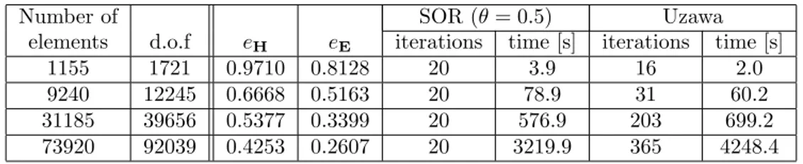
The program has been tested by solving this academic problem with four successively refined meshes, with grid sizes corresponding to h, h/2, h/3 and h/4 and setting the parameter γ equal to one in the four cases. In Table 1 we present the relative error between the computed and the exact solutions. More precisely, we set
eH= 0HC− HC,h0H(curl;ΩC) 0HC0H(curl;ΩC) , eE= 0'EI− 'EI,h0H(curl;ΩI) 0'EI0H(curl;ΩI) .
Figure 1 shows the plots in a log–log scale of the relative errors of eH and eE versus the number of degrees of freedom. As can be seen, the error is reduced when the mesh is refined, even though the relative error for the finest mesh is still quite large. One of the reasons for these large errors is that the solution of our problem is a polynomial of seventh degree, and the support is concentrated in a small part of the domain.
Number of SOR (θ = 0.5) Uzawa
elements d.o.f eH eE iterations time [s] iterations time [s]
1155 1721 0.9710 0.8128 20 3.9 16 2.0
9240 12245 0.6668 0.5163 20 78.9 31 60.2
31185 39656 0.5377 0.3399 20 576.9 203 699.2
73920 92039 0.4253 0.2607 20 3219.9 365 4248.4
Table 1: Results for problem with known analytical solution.
In Table 1 are also presented the number of iterations and computational times when solving system (16) using
SOR method with relaxation parameter θ = 0.5 and when solving with Uzawa’s method. In this case, since ΩI is
simply connected, the perturbation parameter in the SOR method can be taken ε = 0 and the number of iterations is independent on the mesh size. The computational time includes the calculation of the preconditioners.
103 104 105 106 10−0.7 10−0.6 10−0.5 10−0.4 10−0.3 10−0.2 10−0.1 Number of d.o.f. Relative errors Rel. error H C Rel. error E I y=Ch
Figure 1: Relative error versus number of d.o.f.
Two tori
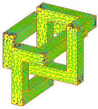
In the second test the computational domain is a cube with edge length 27 cm. We consider two coaxial tori of square section with edge length 1 cm. and radius 6.5 cm. (see Figure 2 where a similar torus is shown):
the upper torus is a coil, that is part of the insulator region ΩI, where we impose a clockwise current density
Je,I of magnitude 106 A/m2, whereas the second torus is the conductor. For the physical magnitudes we are
taking µ = µ0= 4π × 10−7 H/m, the magnetic permeability of the air, σ = 107S/m and the angular frequency
ω = 2π× 50 rad/s. The parameter γ is set equal to 106.
In this case, since the air region ΩI is not simply connected, the parameter ε in the SOR method must
be positive. We present in Table 2 the convergence results for different choices of ε and θ for a mesh with
27152 elements. Then we take the best values found for both parameters (θ = 0.5, ε = 105) and use them in
three different meshes to compare the behaviour of the modified SOR and the Uzawa’s method. The results are summarized in Table 3.
ε = 105 ε = 106 ε = 107 iterations time [s] iterations time [s] iterations time [s]
θ = 0.25 51 720.8 196 1392.2 1751 6372.1
θ = 0.5 22 461.9 96 761.3 874 3247.5
θ = 0.75 NC NC 63 580.6 582 2251.1
θ = 1 NC NC 47 496.3 436 1760.4
θ = 1.25 NC NC NC NC 357 1505.0
Table 2: Two tori. Results for the SOR method with several values of θ and ε. (NC: not convergent)
Number of SOR (θ = 0.5, ε = 105) Uzawa
elements d.o.f iterations time [s] iterations time [s]
3394 4763 24 32.8 336 55.6
27152 34795 22 461.9 239 751.3
91638 113853 25 2937.1 211 4356.1
Table 3: Two tori. Comparison of SOR and Uzawa’s method. The trefoil knot
We want to show how the (HC, 'EI) formulation performs in problems with complicated geometries, (see
Re-mark 2.1). In particular we consider a problem in which the conductor is a socalled trefoil knot. It is well
known (see e.g. [5], [7] ) that there exists one “cutting” surface which cuts any non-bounding cycle in ΩI, but its
construction is a difficult task.
We suppose that ΩC is a trefoil knot formed joining cubes of edge length 1 cm. Above the conductor there
is placed a torus-shaped coil (see Figure 2). The sizes of the coil and the computational domain Ω are the same that in the previous test case. The physical magnitudes, the source current and the parameter γ are also taken as in the two tori test case.
Figure 2: Detail of the mesh for the trefoil knot
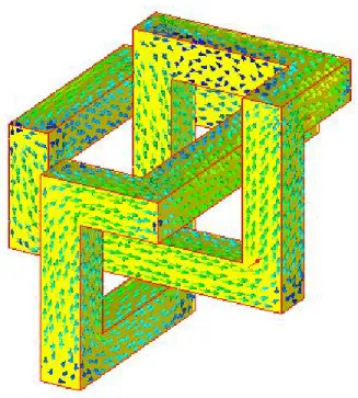
In Table 4 we present the number of iterarions and the CPU time for the modified SOR method with relaxation
part and the imaginary part of the current density JC= curl HC on the surface of the knot.
Number of SOR (θ = 1, ε = 106) Uzawa
elements d.o.f iterations time [s] iterations time [s]
37057 51665 402 4524.4 678 5673.4
Table 4: Results for the trefoil knot.
Figure 3: The current density in the trefoil knot: real part Benchmark problem 7 in the TEAM Workshop
Our last test corresponds to benchmark problem number 7 in the TEAM workshop (see [6]). It consists of a thick aluminum plate with a hole eccentrically placed, and subjected to an asymmetric magnetic field. The field is produced by an exciting current traversing a coil above the plate (see Figure 5). The magnetic permeability is
µ = 4π× 10−7 H/m, the electrical conductivity is σ = 3.526 × 10⁷ S/m, the angular frequency is ω = 2π × 50
rad/s, and the absolute value of the real part (respectively, imaginary) of the excitation current density Je,I is
1.0968 × 10⁶(respectively 0) A/m2. The parameter γ is set equal to 5 × 10⁶.
In Table 5 we present the number of iterations and CPU time for the perturbed-SOR method with relaxation
parameter θ = 1 and ε = 106, and for the Uzawa’s scheme.
Number of SOR (θ = 1, ε = 106) Uzawa
elements d.o.f iterations CPU time [s] iterations CPU time [s]
98857 131434 134 16868.6 191 17794.4
Figure 4: The current density in the trefoil knot: imaginary part 19 30 100 X Z 0 34 19 A1 A3 B3B1 288 Y X 0 108 150 18 150 108 18 294 294 R25 R50 288 A1 B1 (A3) (B3) 72
Figure 5: Geometry of the TEAM model
We also present a comparison of our numerical results with the experimental data given in [6]. In the left
of Figure 6 is represented the z component of the magnetic induction BI (≡ ωi curl 'EI) along a straight line in
the air region, with y = 72 mm. and z = 34 mm. In the right of Figure 6 is represented the y component of
z = 19 mm. We notice that the results for the magnetic induction in the air are not completely satisfactory. This
is due to the fact that BI is calculated from the curl of the computed 'EI and since we are using first order edge
elements this curl is constant on each element. The oscillations are due to the relative position of the elements of the mesh where we compute the numerical values, with respect to the line where the field is measured.
0 0.05 0.1 0.15 0.2 0.25 0.3 −40 −20 0 20 40 60 80 100 x (m) sign(Re(B z ))|B z | (G) numerical experimental 0 0.05 0.1 0.15 0.2 0.25 0.3 −2 −1.5 −1 −0.5 0 0.5 1 1.5 2x 10 6 x (m) sign(Re(J y ))|J y | (A/m 2) numerical experimental
Figure 6: Left: z component of BI along line A1–B1. Right: y component of JC along line A3–B3.
5
Conclusions
We have implemented the finite element approximation of the HC/EI formulation of the eddy-current problem
studied in [2]. In particular we have considered a reduced linear system eliminating the Lagrange multiplier introduced in the insulator region by the penalty method. For the resolution of the resulting linear system we have proposed two different algorithms: a modified SOR method and an Uzawa-like scheme. Both algorithms take advantage of the coupled nature of the eddy current problem, which distinguishes between a conductor and an insulator.
In the light of the results presented above, the modified SOR method performs better in all the four test cases. The number of iterations by subdomains is smaller than for the Uzawa’s method and also the CPU time is lower. In our opinion the performance of Uzawa’s method can be improved with a better preconditioner for the matrix
P defined in (19).
In the case of a simply connected conductor the penalization parameter of the modified SOR method is taken
ε = 0 (so the method is actually the standard SOR), and the rate of convergence turns out to be independent
of the mesh size. In other geometrical situations ε must be positive, and the performance of the modified SOR method depends on the choice of this ε and the relaxation parameter θ.
Morever it is worthy to note that the condition number of the reduced system is quite sensible to the choice of the penalization parameter γ.
Acknowledgements. It is a pleasure to thank Oszk´ar B´ır´o and Alberto Valli for some useful conversations about the subject of this paper.
The second author (R.V.H.) has received financial support by a predoctoral grant FPI from the Spanish Ministry of Education and Science, cofinanced by the European Social Fund.
References
[1] A. Alonso Rodr´ıguez, P. Fernandes, and A. Valli, Weak and strong formulations for the
pp. 387–406.
[2] A. Alonso Rodr´ıguez, R. Hiptmair, and A. Valli, A hybrid formulation of eddy current problems, Numer. Methods Partial Differential Equations, 21 (2005), pp. 742–763.
[3] C. Amrouche, C. Bernardi, M. Dauge, and V. Girault, Vector potentials in three–dimensional
non-smooth domains, Math. Meth. Appl. Sci., 21 (1998), pp. 823–864.
[4] M. Benzi, G. H. Golub, and J. Liesen, Numerical solution of saddle point problems, Acta Numer., 14 (2005), pp. 1–137.
[5] A. Bossavit, Computational Electromagnetism. Variational Formulation, Complementarity, Edge Elements, Academic Press, San Diego, 1998.
[6] K. Fujiwara and T. Nakata, Results for benchmark problem 7 (asymmetrical conductor with a hole), COMPEL, 9 (1990), pp. 137–154.
[7] P. W. Gross and P. R. Kotiuga, Electromagnetic Theory and Computation. A Topological Approach, Cambridge University Press, New York, 2004.
[8] Q. Hu and J. Zou, An iterative method with variable relaxation parameters for saddle-point problems, SIAM J. Matrix Anal. Appl., 23 (2001), pp. 317–338 (electronic).
[9] , Substructuring preconditioners for saddle-point problems arising from Maxwell’s equations in three
dimensions, Math. Comp., 73 (2004), pp. 35–61 (electronic).
[10] H. Kanayama, D. Tagami, M. Saito, and F. Kikuchi, A numerical method for 3-D eddy current