Feasibility study and development of a full digital passive radar demonstrator

(1)

UNIVERSITÀ DI PISA

Scuola di dottorato in Ingegneria “Leonardo da Vinci”

Corso di Dottorato di Ricerca in

TELERILEVAMENTO

Tesi di Dottorato di Ricerca

“Feasibility study and development of a full digital passive radar

demonstrator”

Autore

Relatori

Michele Conti

__________________

Prof. Marco Martorella

___________________

Dr. Ing. Amerigo Capria

____________________

(2)

A

BSTRACT

In the past few years we have witnessed a growing interest in Passive Radars which exploit electromagnetic emissions coming from non-cooperative transmitters for example TV/Radio stations. The main feature of these systems is the absence of a transmitter. This feature, in addition to reduced system costs, makes this kind of equipment hard to intercept.

Many demonstrators have been developed in the past decade by Universities, research facilities and private companies, however, we can’t say we have found a solution to fully satisfy the performance and cost requirements.

This thesis focuses on the development of a low cost passive radar demonstrator with the aim of achieving a high range resolution exploiting the DVB-T signal as illuminator of opportunity (IO), which should satisfy both cost and performance needs.

The study and design of the above mentioned radar demonstrator lead to three main innovative aspects.

The first aspect is the realisation of a low cost passive radar demonstrator based on Software Defined Radio (SDR) technologies. In particular the Universal Software Radio Peripherals (USRPs) seems to be a good solution which meets the requirements of scalability and modularity which our system must have, for example the possibility to receive different signals by using the same hardware configured via software.

The second aspect is the development of the whole processing chain. A theoretical analysis and experimental validation for every algorithm have been done. In particular, all algorithms developed are independent from the type of illuminator of opportunity chosen. This advantage, in conjunction with the use of a hardware which can be reconfigured via software, makes the entire radar system adaptive to the signal used. The third and final point focuses on the way to obtain a passive radar system which offers high range resolution. Specifically, in this thesis, the possibility of obtaining a high range resolution using adjacent DVB-T channels has been studied.

A theoretical analysis, followed by a validation on real data will highlight that the resolution enhancement is proportional to the number of exploited DVB-T channels.

(3)

The radar’s functionality is tested on different scenarios: maritime and aerial. The experimental results obtained with the demonstrator in both scenarios for different types of targets is proved both the feasibility of our radar system and the actual improvement of range resolution resulting from using multiple DVB-T adjacent channels

(4)

A

CRONYMS

ACF Autocorrelation Function

ADC Analog to Digital Converter

ADS-B Automatic Dependent Surveillance - Broadcast

AF Ambiguity Function

API Application Programming Interface

CAF Cross Ambiguity Function

CCF Cross-Correlation Function

CNR Clutter to Noise Ratio

COFDM Coded Orthogonal Frequency-Division Multiplexing

COTS Commercial Off-the-Shelf component

DAB Digital Audio Broadcasting

DBPSK Differential Binary Phase Shift Keying

DDC Digital Down-Converter

DNR Direct to Noise Ratio

DVB-T Digital Video Broadcasting - Terrestrial

EIRP Equivalent Isotropic Radiated Power

FFT Fast Fourier Transform

FM Frequency Modulation

GI Guard Interval

GNU Gnu is Not Unix

GSM Global System for Mobile Communications

IO Illuminator of Opportunity

LAN Local Area Network

LIT Long Integration Times

LNA Low Noise Amplifier

LS Least Squares

MIMO Multiple-Input and Multiple-Output

(5)

OFDM Orthogonal Frequency-Division Multiplexing

PBR Passive Bistatic Radar

PCI Peripheral Component Interconnect

PCL Passive Coherent Location

PCR Passive Covert Radar

PRBS Pseudorandom Binary Sequence

RAID Redundant Array of Inexpensive Disks

RDA Range-Doppler-Azimuth

RF Radio Frequency

SDR Software Defined Radio

SFN Single Frequency Network

SINR Signal Interference plus Noise Ratio

TPS Transmission Parameters Signalling

UHD Universal Hardware Driver

UHF Ultra High Frequency

UMTS Universal Mobile Telecommunications System

USB Universal Serial Bus

USRP Universal Software Radio Peripheral

VHF Very High Frequency

Wi-Fi Wireless Fidelity

WiMAX Worldwide Interoperability for Microwave Access

(6)

L

IST OF

F

IGURES

Figure 1.1 Passive Radar Concept ... 14

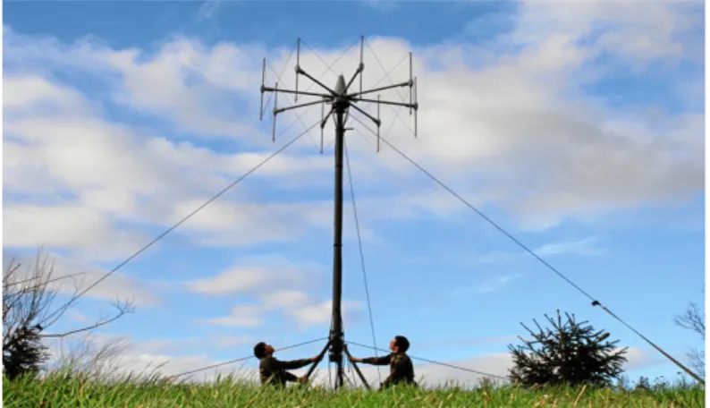
Figure 1.2 PaRaDe II: antenna array (left) and beam pattern (right)... 17

Figure 1.3 PaRaDe II: receiving chain... 17

Figure 1.4 Cora antenna array: the lower panel is designed for DAB reception (red rectangle) and the upper one for DVB-T reception (blue rectangle)... 18

Figure 1.5 Cora system architecture ... 19

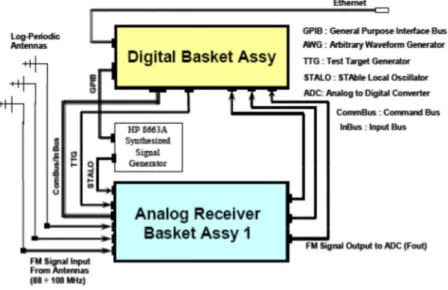
Figure 1.6 BAE system architecture ... 20

Figure 1.7 Homeland Alerter 100 ... 21

Figure 1.8 Aulos block diagram (left)and system (right) ... 23

Figure 1.9 Aulos receiver architecture... 23

Figure 1.10 Silent Sentry system ... 24

Figure 1.11 Cassidian system concept and architecture ... 25

Figure 1.12 Cassidian system multiband antenna... 26

Figure 1.13 Bistatic radar geometry ... 27

Figure 1.14 Signal Processing Chain for Passive Radar... 31

Figure 2.1 Geometry for bistatic range resolution... 35

Figure 2.2 Geometry for bistatic Doppler resolution... 36

Figure 2.3 DVB-T transmission system ... 37

Figure 2.4 OFDM signal consists of several narrow sub-carriers ... 37

Figure 2.5 Pilot structure in the DVB-T OFDM frame ... 39

Figure 2.6 Guard Interval in OFDM symbol ... 39

Figure 2.7 DVB-T simulator... 40

Figure 2.8 DVB-T spectrum ... 40

Figure 2.9 Ambiguity function of DVB-T signal ... 41

Figure 2.10 Multichannel DVB-T Spectrum ... 43

Figure 2.11 Single and Multichannel DVB-T Ambiguity Function... 44

Figure 2.12 Single and Multichannel DVB-T Ambiguity Function (Zoom View) ... 44

(7)

Figure 3.1 Reference Signal Pre-processing block... 47

Figure 3.2 General block diagram of a DVB-T receiver ... 48

Figure 3.3 Sketch of LS batches algorithm... 54

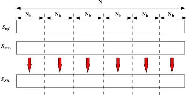
Figure 3.4 Reference and surveillance signals segmentation ... 58

Figure 3.5 Reference and surveillance signals segmentation ... 59

Figure 3.6 Multiple DVB-T channel combination scheme... 60

Figure 4.1 Reference signal constellation before and after reconstruction for every channel ... 62

Figure 4.2 Effectiveness of the signal reconstruction (range profile). Circles show multipath peaks ... 63

Figure 4.3 Effectiveness of the signal reconstruction (range profile). Zoom for negative delays ... 63

Figure 4.4 Effectiveness of the signal reconstruction (range profile). Zoom for positive delays ... 64

Figure 4.5 Reference signal Ambiguity Function before equalization... 64

Figure 4.6 Cross Ambiguity Function between reference signal after equalizing and reference signal ... 65

Figure 4.7 Target representation of the reference scenario ... 67

Figure 4.8 Range Doppler Map before direct signal and clutter cancellation ... 67

Figure 4.9 Range Doppler Map after LS filtering ... 68

Figure 4.10 SINR values of each targets after NLMS filtering for different weight vector ... 69

Figure 4.11 SINR values of each targets after LS filtering for different weight vector . 69 Figure 4.12 Time processing elapsed for LS (red line) and NLMS (blue line) filtering 70 Figure 4.13 Time processing elapsed for Direct FFT method and batch algorithm... 72

Figure 4.14 Losses of the target power averaged with respect to the Doppler frequencies ... 73

(8)

Figure 5.4 a) Surveillance Antenna b) Radiation Pattern for 95 elements antenna at

different frequencies ... 79

Figure 5.5 a) Reference Antenna b) Radiation Pattern for 47 elements antenna at different frequencies ... 79

Figure 5.6 Signal Processing scheme ... 80

Figure 5.7 DVB-T Passive Radar Demonstrator Equipment... 81

Figure 6.1 DVB-T Passive Radar Demonstrator ... 82

Figure 6.2 Experiment Scenario geometry and target trajectories (Aerial Scenario)... 83

Figure 6.3 Doppler frequencies calculated exploiting the ADS-B data (velocity, heading and position of the target) as a function of the target azimuth position respect to the receiver... 84

Figure 6.4 Main technical information of the detected target... 84

Figure 6.5 CAF of the surveillance area ... 85

Figure 6.6 Target range profile for a single DVB-T channel (dashed line on the top) and for three adjacent DVB-T channels (solid line on the bottom)... 86

Figure 6.7 Experiment Scenario geometry and target trajectories (Maritime Scenario) 87 Figure 6.8 Surveillance Area ... 88

Figure 6.9 Expected Doppler frequencies for ships departing from the nearby harbor (receding from receiver) ... 88

Figure 6.10 Surveillance area during the acquisition ... 89

Figure 6.11 DVB-T CAF of the surveillance area... 89

Figure 6.12 Target range profile for a single DVB-T channel (blue line on the top) and for three adjacent DVB-T channels (red line on the bottom) ... 90

(9)

L

IST OF

T

ABLES

Table 1.1 Summary of typical parameters of PBR illuminator of opportunity ... 30

Table 4.1 Numerical Evaluations of the attenuations ... 65

Table 4.2 Target echoes parameters for the reference scenario... 66

Table 4.3 SINR values after LS filter (last column) ... 70

Table 5.1 SDR boards/subsystem providers ... 74

(10)

I

NTRODUCTION

Passive Bistatic Radar (PBR, also referred to as Passive Coherent Location) exploits Illuminators of Opportunity (IO) such as FM radio, DAB, analogue and digital television signals, GSM/UMTS base stations in order to detect and track targets. This system concept is of great interest in both civilian and military scenarios mainly due to number of advantages offered by this system with respect to active radar. A PBR system may benefit from an enhanced target Radar Cross Section (RCS) with respect to the monostatic case, thanks to the lower frequency of operation (i.e.: VHF and UHF bands) and the bistatic configuration. Moreover, it does not require any dedicated frequency band allocation, it allows covert surveillance and it can be developed with a reduced budget using low cost components thanks to the absence of the transmitter unit. This radar technology may also be realized by means of Software Defined Radio systems, which typically meet low cost requirements and guarantee system flexibility. The performance of a passive radar system strongly depends on the transmitted power and on the characteristics of the exploited IO, which is used as a reference signal. As the range coverage increases when the transmitted power level increases, high-power transmitters, such as broadcast FM, DAB radio, analogue and DVB television transmitters, are preferable.

Furthermore, in many countries, analogue radio and TV transmissions will be soon dismissed and will be replaced by digital ones. In summary, DVB-T transmitters should be considered to be one of the best candidates for passive radar purposes thanks to the high level of radiated power and to the good waveform performances in terms of range and Doppler resolution.

An ongoing research field about passive radar systems concerns the theoretical range resolution improvement achieved by using multiple FM channels and DVB-T channels. In this thesis, the possibility to improve the range resolution by using multiple adjacent DVB-T channels from the same transmitter will be addressed.

In this thesis a DVB-T Software Defined Passive Radar demonstrator will be developed, the whole processing chain will be described and tested. The hardware of the

(13)

Then the range resolution improvement will be obtained by considering multiple adjacent DVB-T channels as a single wideband signal. Furthermore experimental results obtained with our demonstrator in two different scenarios will be shown. The effective improvement on the range resolution will be underlined by comparing the results obtained for a single and multiple DVB-T channel operation.

(14)

Chapter 1. P

ASSIVE

B

ISTATIC

R

ADAR

S

YSTEMS

1.1. P

RINCIPLE

Passive Bistatic Radar (PBR) systems, also referred to as Passive Coherent Location (PCL) systems, exploit reflection from illuminators of opportunity (IO) in order to detect and track objects. A PBR receiver, as shown in Figure 1.1 , generally presents two receiving channels [1] denoted as reference channel and surveillance channel. The reference channel is used to capture the direct signal from the transmitter and provides a reference signal to be compared with the target return.

Figure 1.1 Passive Radar Concept

Transmitter Satellite Reference Antenna Surveillance Antenna Reference Channel Target Channel Baseline

(15)

The comparison is usually carried out by a cross-correlation [2] between reference signal and the target signal and it actually represents the basic process to detect targets with a passive radar.

The application area of passive radars is strictly dependent on the illuminator of opportunity properties [3]. The important features of an illuminator of opportunity are: the power density values at the target, the coverage, the signal characteristics and its ambiguity properties.

The illuminators of opportunity can be divided into two main classes: analogue emitters like FM radio [4]-[6], analogue TV, or digital transmitter as DAB/DVB-T [7],[8], GSM [9], UTMS [10], Wi-Fi, WiMAX [11]. Passive radars based on analogue signals show detection performance strongly dependent on the signal content. In contrast, digital waveforms, thanks to specific signal coding, have spectral properties which are nearly independent of the signal content.

The most effective mathematical tool used for studying the radar performances of a given waveform is the ambiguity function (AF), mathematically defined as:





2 2 _* ( , )f_d s t s t( ) ( ) exp 2j f t dt_d       



 (1.1)

where is the complex envelope of the transmitted signal, is the time delay and

is the Doppler frequency shift. The AF cross-section at is the signal

autocorrelation function (ACF).

By means of the ambiguity function, range and Doppler resolutions are directly obtained.

 

s t 

d

(16)

1.2. S

TATE OF THE ART

As a result of a study of the state of the art, some examples of passive radars are presented. The main characteristics dealing with antenna structure, receiving chains and processing architectures will be described.

1.2.1. PARADE (Passive Radar Demonstrator) Warsaw University of Technology

PaRaDe exploits transmissions from commercial FM radio stations in order to detect and track airborne targets [5],[6].

The antenna system is a circular antenna array composed of eight half-wave dipoles (Figure 1.2). Beamforming coefficients are applied for creating static beams, independently of the received signals. One beam is pointed in the transmitter direction, which is assumed to be known. The rest of beams correspond to the surveillance channels. The signal from each of the surveillance beams is fed to a separate processing chain (Figure 1.3).

The signal from the antennas is amplified, filtered and digitized in RF, without analog down conversion process. The selected radio channel is digitally down converted to the baseband by a quadrature demodulator and the complex IQ samples are sent to a general purpose PC using USB 2.0 interface. The software running on the PC is written in C/C++ and works under Windows or Linux operating systems. It consists of three parts responsible for: data reception, signal processing and visualization.

(17)

Figure 1.2 PaRaDe II: antenna array (left) and beam pattern (right)

Figure 1.3 PaRaDe II: receiving chain

1.2.2. CORA COvert RAdar (FHR)

This system can exploit alternatively Digital Audio Broadcasting (DAB) or Digital Video Braodcasting-Terrestrial (DVB-T) signals, using a circular antenna array with elements for the VHF (150-350 MHz) and the UHF-range (400-700 MHz). A fiber optic link connects the elevated antenna and RF-frontend with the processing back-end, consisting of a cluster of high power 64 bit-processors [7],[12].

(18)

DAB reception. The 16 elements, feeding the 16 receiver channels of the front-end, allow 360° beamforming.

 A half of the upper plane is equipped with 16 vertically polarized UHF-broad band dipoles for DVB-T reception, to allow for 180º beamforming. The other half of the upper plane is equipped with spare dipole elements.

 Alternatively, both planes can be equipped with crossed butterfly dipoles, which can be combined to sharpen the beam in elevation.

Figure 1.4 Cora antenna array: the lower panel is designed for DAB reception (red rectangle) and the upper one for DVB-T reception (blue rectangle).

The Cora system architecture is presented in Figure 1.5:

 The RF-front-end consists of 16 equal receiver channels, composed of a Low-Noise Amplifier (LNA), a tunable or fixed filter and an adaptive gain control for optimum control of the ADC.

 A chirp signal generated by a separate signal generator and transmitted to the front-end by coaxial cable, is used for calibration. A bank of switches provides for calibration of each receiver channel chain from the LNA to the ADC, excluding only the antenna element.

(19)

 A/D conversion is realized with 4 FPGA boards. Each boards is equipped with 4 ADC modules with 14 bit 100 Msamp/sec maximum sample rate ADC-chips, for processing 4 receiver channels. Each FPGA provide an output channel.  Each ADC output is fed to an electro-optic converter and linked to the signal

and data processing unit via a fiber-optic cable. In the signal and data processing unit, the optical signals are converted back to digital data streams of 4 serial channels, each, using 64-bit-boards, hosting 4 FPGAs. Four high performance Quad-Opteron computers handle the four data streams.

(20)

1.2.3. MULTIBAND Passive Radar Demonstrator, BAE System

This is a four-channel system capable of receiving and processing analogue and digital transmissions over a band covering 200MHz to 2GHz, providing sufficient bandwidth to process the analogue and digital transmissions of interest [13]. The system architecture is presented in Figure 1.6.

Figure 1.6 BAE system architecture

The antenna system consists of an array of four wideband Log-Periodic Dipole antennas, at a 45° angle from vertical to permit joint reception of vertically and horizontally polarized signals, with some loss. Additional, high gain, antennas were used for obtaining transmitter signal references.

The system incorporates near-instantaneous RF switching between one of several RF filters for true multiband system operation, under PC software control. The system was designed to operate on one of four channels. In the configuration reported in [13] a DAB channel and three DVB-T channels might be processed.

(21)

For reducing the DPI impact, analogue suppression of the direct signal at the element level was implemented. The reference signals were applied to vector modulators for obtaining anti-phase reference signals for addition to the main channel signals. The modulators were under PC control.

For data acquisition on a PC, an ICS-645-4A 32-bit 33MHz PCI card was selected. This provides four onboard ADCs clocked at up to 20MHz. A RAID array with dedicated raid controller card, multiple PCI buses, and enhanced data capture software enabled the required 80MB/sec (four channels at two bytes per channel and at 10MHz rate).

1.2.4. HOMELAND ALERTER 100 (THALES)

The Homeland Alerter 100 (Figure 1.7) is a passive radar sensor using illuminators of opportunity provided by FM radio broadcasts. Possible extension with DAB (Digital Audio Broadcast), AVB (Analog Video Broadcast) and DVB-T (Digital Video Broadcast –Terrestrial).

Figure 1.7 Homeland Alerter 100

The main characteristic of the system are :  Detection performances on 360°:  Range: class 100 km

(22)

 Configurable for mobile platforms or fixed sites:

 Commercial or 4x4 military vehicle (using car driver licence)  Stand alone or in network operations

 Connection to Command and Control Centers through Asterix/AWCIES protocol

 Delivered with a software (Aneth) for deployment support and performance prediction

The Homeland Alerter 100 has already been sold to several NATO countries.

1.2.5. AULOS (Passive Covert Location Radar) Selex Sistemi Integrati

In [4], the design, development and test of a Passive Covert Radar (PCR), exploiting a single non co-operative FM commercial radio station as its transmitter of opportunity are described. In Figure 1.8 the block diagram and the system are presented. The reference signal is collected by a single antenna. The surveillance system is composed of two antennas with independent receiving and processing chains. A “2/2 logic” is

applied to extract the detections common to both channels, with cell tolerance in

Doppler. Target bearing is estimated using a simple phase interferometry.

The receiver architecture is shown in Figure 1.9. In the analog section two down conversions are applied:

 The former lowers the carrier to the first IF and selects the FM channel of interest.

 The latter amplifies and moves the signal to the second IF.

This signal will be filtered, amplified and acquired by the A/D converter with 10 MSps clock frequency. Digital Down Conversion (DDC) is finally applied to obtain the complex signal digital components handled by signal and data processor.

The digital processing section, is running on three Intel® Core™2 PCs, connected via LAN.

1 

(23)

Figure 1.8 Aulos block diagram (left)and system (right)

Figure 1.9 Aulos receiver architecture

1.2.6. SILENT SENTRY

The Silent SentryTM2 (SS2) system (Figure 1.10) is a receive system that exploits transmission from multiple commercial FM radio stations to passively detect and track airborne targets in real-time. On 10 May 1999,, Silent Sentry received Aviation Week & Space Technology magazine's Technology Innovation Award, which recognizes innovative product and service technologies in the global aerospace business.

(24)

Figure 1.10 Silent Sentry system

Silent Sentry is a single receive system composed primarily of the following components the majority of which are commercial off-the shelf (COTS):

 Target array: a linear phased array for detecting the scattered energy from targets in the region of interest

 Reference Antennas: single element, identical to those in the target array, used for reception of the direct path signal from FM illuminators

 High Dynamic Range Receivers: accommodate the dynamic range requirements for receiving direct and scattered signals simultaneously.

 A/D Converters: the system possesses the capability to record data at this level, which is particularly useful for post-mission analysis

 Processor: Silicon Graphics, inc (SGI) general purpose processor

 Displays: SGI Octane workstations and visualizations products from the

Autometric Edge Product FamilyTM.

 High Speed Tape System: a SCSI attached striping tape controller with 5 tape drivers

Lockheed Martin currently has two configurations of SS2: the Fixes Site System (FSS) and the Rapid Deployment System (RDS).

1.2.7. CASSIDIAN MULTIBAND MOBILE Passive Radar System

In [14] a passive system capable of processing DVB-T SFN, DAB-SFN and 8 FM channels simultaneously is proposed. The architecture of the system is presented in Figure 1.11.. In this system, all the signals are digitally down converted according to the

(25)

software defined radio concept. The antenna system is depicted in Figure 1.12. It is composed of the following sub-systems:

• A 2x7 element planes covering the frequency band that ranges from 474 MHz to

850 MHz (DVB-T antenna), which allows 3D bearing.

• A 1x7 array covering the frequency range from 88 MHz to 240 MHz (FM/DAB

signals), which allows 2D bearing.

• Auxiliary elements: a lightning, compass and calibration units.

In [14] only FM measurements are reported.

(26)

(27)

1.3. B

ISTATIC

R

ADAR 1.3.1. Bistatic radar Geometry

Figure 1.13 shows the bistatic geometry [15]. the transmitter and receiver are separeted by the baseline L. The angle subtended at the target by the transmitter and receiver is

the bistatic angle, . there are essentially three parameters that the bistatic receiver

may measure:

I. The difference in Range between the direct signal and the

transmitter-target-receiver path

II. The angle of arrival of the received echo

III. The Doppler shift of the receive echo

Figure 1.13 Bistatic radar geometry





RT RRL



R  d f

Transmitter baseline Receiver L T  R T R R R target T R    N 2  is orange contour (ellips e)

(28)

Contours of constant bistatic range define an ellipse, with the transmitter and

receiver at the two foci. If and are measured and is known, the range

of the target from the receiver may be found from:

(1.2) In the general case when transmitter, target and receiver are all moving, the Doppler shift on the echo is obtain from the rate of change of the transmitter target receiver path. If the transmitter and receiver are stationary, the Doppler shift on the received echo is given by:

(1.3)

where is the target velocity and is the angle of the velocity with respect to the

bisector of the bistatic angle .

1.3.2. Radar Equation

The starting point for prediction of PBR performance is the bistatic radar equation: (1.4) where

is the receive signal power is the transmit power

is the transmit antenna gain is the transmitter-to-target range is the target bistatic radar cross-section

is the target-to-receiver range is the receiver antenna gain is the radar wavelength



RT RR





RTRR



R L





 





2 2 2 sin T R R T R R R R L R R R L      

  



2 cos cos 2 d v f     v   2 2 2 1 4 4 4 t t r r b T R PG G P R R          r P t P t G T R b  R R r G 

(29)

The signal-to-noise ratio is obtained by dividing (1.4) by the receiver noise power

(where is Boltzmann's constant, is 290 K, is the receiver

bandwidth and the receiver noise figure), and multiplying by the receiver processing

gain, also taking into account the various losses.

The factor in eq. (1.4) means that the signal-to-noise ratio has a minimum

value for , and is greatest when the target is either close to the transmitter or

close to the receiver. Contours of constant values of , and hence of

signal-to-noise ratio, define geometric figures known as Ovals of Cassini [15].

In predicting the detection performance of a PBR system it is critical to understand the correct value of parameters to insert into this equation. In particular, it must be appreciated that the ambient noise level will be high, particularly in the VHF and UHF bands, and particularly in urban enjoinments, due the direct signal, co-channel signals, spectral 'slop', multipath, and noise. This means that dynamic range of PBR receiver will need to be substantial to cope with the wide range of the signal levels (typically >90dB) 0 n P kT BF k T₀ B F 2 2 1 T R R R       T R R R 2 2 1 T R R R      

(30)

1.4. T

YPICAL ILLUMINATORS

Quite evidently, PBR depends upon the use of waveforms that are not explicitly designed for radar purpose. In Table 1.1, the main parameters of a number of different types of waveform are reported.

Signal of opportunity Frequency (MHz) EIRP (KW) Instantaneous Bandwidth (MHZ) Monostatic Range Resolution (m) FM 87.5-108.0 250 0.16 937 (variable) GSM 935-960 1805-1880 0.01-0.1 0.2 750 UMTS 2110-2170 0.001-0.1 3.84 39 DAB 174-240 1452-1490 0.8-1.6 1.536 100 DVB-T 164-860 0.1-10 7.61 19.7 Wi-Fi 802.11 2400 0.0001 5 30 Wi-MAX 802.16 2400 0.02 20 15

Table 1.1 Summary of typical parameters of PBR illuminator of opportunity

To summarize, there is a wide variety of different types of source that might be used for PBR purpose. The parameter that need to be taken into account in assessing their usefulness are:

I. their power density at the target

II. their coverage (both spatial and temporal)

III. the nature of their waveform

In general, digital modulation schemes are found to be more suitable than analog, since their ambiguity function properties are better (since the modulation is more noise-like),

(31)

Among digital waveform the best compromise between range resolution and EIRP value can be achieved by using DVB-T signals.

In the next chapters we will show how a DVB-T based Passive Radar High Range Resolution can be achieved by jointly using adjacent multiple channels transmitted by the same IO.

1.5. P

ROCESSING

C

HAIN

A general block scheme of a passive radar system is sketched in Figure 1.14

Digital Beamforming Reference

Channel

Surveillance Channel

Pre-processing ZDI Suppresion

2-D Matched Filter

(32)

A complete passive radar system typically consist of the following processing steps:  Digital Beamforming: we can summarize the main goals of the digital

beamforming in array passive radar as follow:

 Reference channel beamforming: it is used to form the direct signal beams on the direction of the transmitters of opportunity that we intend to use for implementing passive radar functionality. Ideally the reference beam attempts to minimize the corruption in the transmitted waveform estimate caused by the superposition of unwanted signal multipath components.

 Surveillance channel beamforming: it is used to form one or more surveillance beams in pre-determined directions selected for target search. Ideally the surveillance channel provides the maximum gain for target echoes while cancelling all interference components. A solution with multiple beams seems to be more practical since it provides higher gain and potential capability of the direction of the arrival estimations.  Pre-processing block: it is used to remove spurious peaks of the radar

ambiguity function caused by deterministic and pseudo-random pilot tones of the waveform

 Zero Doppler Interference suppression: is used to filter out the direct path interference, its multipath and the ground clutter, which are all characterized by a zero Doppler spectrum in the Range- Doppler domain

 2-D Matched Filter: it is used to generate the range- Doppler maps for each input channel, to determine target bistatic range and Doppler. This block represents the key processing step in a passive radar.

 Detector: it is used to detect targets in the 3D Range-Doppler -Azimuth (RDA) domain

 Tracker: it is used to reconstruct the path of targets in the 3D- RDA domain In this thesis we developed only three signal processing blocks, specifically, Pre-processing, Zero Doppler Interference and 2D Matched Filter.

(33)

Chapter 2. A

MBIGUITY

F

UNCTION

A

NALYSIS

2.1. T

HEORETICAL

B

ACKGROUND

Range and Doppler resolution are fundamentally important parameters in the design of any radar system as they govern the ability to distinguish between two or more targets by virtue of spatial or frequency (i.e. radial velocity) differences. The classical way of evaluating the behaviour of a waveform for radar purpose is the ambiguity function. In PBR, and more generally in bistatic radar, the relative positions of target, transmitter and receiver govern the actual resolution that can be achieved. Here we used the formulation derived by Tsao et al. [16] to compute the bistatic ambiguity function:

(2.1)

where

 and are the hypothesised and actual ranges (delays) from the receiver

to the target

 and are the hypothesised and actual target radial velocities with respect

to the receiver

 and are the hypothesised and actual Doppler frequencies

 and as defined in Figure 1.13

























2 2 * , , , , , , , , , exp 2 , , , 2 , , , RH Ra H a R t a Ra R t R RH R DH RH H R Da Ra a R R R V V L s t R L s t R L j f R V L j f R V L t dt                   _  _



RH R R_Ra H V V_a DH f f_Da R  L

(34)

The ambiguity function can lose all range and Doppler resolution if a target is on or close to the transmitter-receiver baseline. for targets at long ranges the form of the ambiguity diagram is much like that for the monostatic case. These represent the two extremes, practical cases lie in between the two.

2.1.1. Bistatic Range Resolution

The bistatic range resolution can be calculated as the minimum distance between two targets that guarantees a time delay between their respective radar echoes equal to

, where is the velocity of light and the signal bandwidth. In Figure 2.1 an example

of a bistatic geometry is presented with three targets. Target 1 and Target 2 are collinear

with the bistatic bisector, whereas target 3 present an aspect angle . To generate

separation at a bistatic receiver, two point scattering targets, such as Targets1 and

2 in Figure 2.1, must lie on bistatic isorange contours having a separation, , that is

approximately .

When a line joining the two targets is not collinear with the bistatic bisector, but at an

aspect angle with respect to the bistatic bisector, such as for Targets 1 and 3 in

Figure 2.1, their physical separation must be approximately . Hence

the expression that allows the calculus of this parameter is presented in (2.2) where

bistatic is the bistatic angle and is the aspect angle with respect to the bistatic

bisector [17]:

(2.2)

The value obtained for is usually used for specifying the bistatic range resolution

of a system as a function of the bistatic angle.

2 c B c B  2 c B B R 







2 cos 2



c B   R  R_B cos

 

  



  

2 cos / 2 cos c R B     0  

(35)

Figure 2.1 Geometry for bistatic range resolution

2.1.2. Bistatic Doppler Resolution

For monostatic and bistatic Doppler resolution, an adequate degree of Doppler separation between two targets echoes at the receiver is conventionally taken to be

where is the receiver's coherent processing interval. Thus the requirement for

Doppler resolution is

(2.3) where again, the equality represents a minimum requirement for Doppler separation. In the bistatic case the bistatic target Doppler is defined as

to TX to RX Target 1 2  Target 2 isorange contours (ellipses)  Bistatic bisector (with res pect to

Target 1) Target 3 B R  R_  int 1 T Tint 1 2 int 1 Tgt Tgt f f T  



2

   

cos cos 2



f  V   

(36)

The geometry for , , e is shown in Figure 2.2 . The two targets are assumed to be co-located so that they share a common bistatic sector. Combining (2.3) and (2.4) yields

(2.5)

where is the required difference between the two target velocity vectors, projected

onto the bistatic bisector, for adequate bistatic Doppler resolution. When ,

, the monostatic case.

Figure 2.2 Geometry for bistatic Doppler resolution

1 V V₂ ₁ ₂

 









1 1 2 2 int cos cos 2 cos 2 V V V T          _ _ V  0  



2 int



V  T   TX _RX

Target 1 and Target 2

2 

Bistatic bis ector

2  1  2 V 1 V

(37)

2.2. DVB-T W

AVEFORM

A

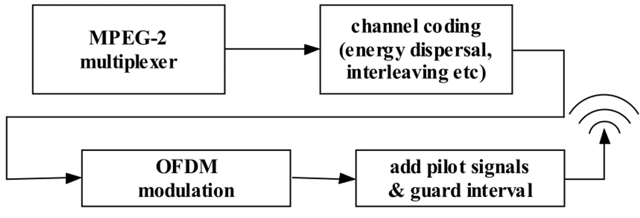
NALYSIS

Figure 2.3 shows the simplified block diagram of a DVB-T transmission system. The processing applied to the output transport stream of an MPEG-2 multiplexer consists of error coding interleaving and orthogonal frequency division multiplexing (OFDM). The combined processing is abbreviated as COFDM.

Figure 2.3 DVB-T transmission system

In OFDM, a wide frequency channel is divided into several sub-carriers that have relatively narrow frequency bandwidth (as shown in Figure 2.4).

The number of sub-carriers is important because the higher the number of sub-carriers spanning a fixed channel bandwidth, the narrower the spacing (bandwidth) of the sub-carriers. Hence, when 64 carriers are used in a 20 MHz channel, the sub-carrier spacing is 312.5 kHz, but when 2048 sub-carriers span the 20 MHz, the spacing is 15 kHz.

MPEG-2

multiplexer

channel coding

(energy dispersal,

interleaving etc)

OFDM

modulation

add pilot signals

& guard interval

(38)

The sub-carrier spacing (or bandwidth) is important as the time domain OFDM symbol

duration is the inverse of the sub-carrier spacing ( ). Hence, for the case of 64

carriers of 312.5 kHz, the symbols duration is , whereas in the case of 2048

carriers of 15 kHz it is .

The wireless propagation channel causes impairments to the transmitted signal. The width of the sub-carrier and duration of the OFDM symbol have direct role in mitigating these impairments. Long symbols and narrow sub-carriers are better suited for a channel that has long stability in time but varies quickly in the frequency domain whereas short symbols and wide sub-carriers are better suited for the case where the channel is highly varying in time yet relatively slowly changing in the frequency domain.

The DVB-T transmitted signal model is expressed in the following equation:

(2.6)

The sub-carriers are separated by within the bandwidth.

The number of sub-carriers depends on the implemented standard. In Italy, 6817

frequency sub-carriers are used, where each sub-carrier is 16 or 64 QAM

modulated with baseband data. The transmitted signal is organized in COFDM frames. Each frame consists of 68 OFDM symbols. Each symbol is formed by a set of data sub-carriers, pilots sub-carriers and transport parameter signalling (TPS).

The TPS carriers convey information about the parameters of the transmission scheme. The carrier locations are constant and defined by the standard and all carriers convey the same information using Differential Binary Phase Shift Keying (DBPSK). The initial symbol is derived from a Pseudorandom Binary Sequence (PRBS).

The pilot symbols aid the receiver in reception, demodulation, and decoding of the received signal. Two types of pilots are included: scattered pilots and continual pilots. The scattered pilots are uniformly spaced among the carriers in any given symbol. In contrast, the continual pilot signals occupy the same carrier consistently from symbol to symbol. The location of all pilot symbol carriers is defined by the DVB-T standard.

1/ s T  f 3.2 s 66.7 s 1 2 ( ) 0 ( ) ( ) SC N j kf t m k S m k s t   c p t mT e    

 

  1 SC s f  T B_{DVB T}_ 7.61MHz



T_s 896s



(39)

indexed horizontally and symbols are indexed vertically [18]. The pilots are based on a

PRBS and are BPSK modulated at a boosted power level, times greater than that

used for the data and TPS symbols.

Figure 2.5 Pilot structure in the DVB-T OFDM frame

The COFDM symbol presents also a guard interval also called the cyclic prefix, is

added to make sure that the delayed symbols don’t overlap with the following symbol. Otherwise, the delayed symbols will cause what’s termed “inter-symbol interference,” which is self-interference resulting from the effects of the propagation channel.

It is a segment of duration , added at the beginning of the COFDM symbol.

16 9

g

T

g

(40)

This segment is identical to the segment of the same length at the end of the symbol.

The duration of the guard interval ranges from 3% to 25% of .

Figure 2.7 DVB-T simulator

A DVB-T transmission system has been simulated through a Simulink® model, see Figure 2.7. The spectrum of the DVB-T signal is a band-pass spectrum signal with a nearly rectangular envelop, as shown in Figure 2.8.

Figure 2.8 DVB-T spectrum

s

(41)

2.3. DVB-T A

MBIGUITY FUNCTION ANALYSIS

The radar ambiguity function is a 2D autocorrelation function given by eq. (1.1). An example from the simulation is given in Figure 2.9.

Figure 2.9 Ambiguity function of DVB-T signal

Several ambiguities are seen aside from the peak at zero-delay and zero-Doppler. To understand the source of these ambiguities, we must look more closely at the structure of the DVB-T signal, namely the pilot signals inserted into the OFDM structure.

The spacing of the scattered pilots is constant within a symbol. Scattered pilots are placed every twelve carriers. For the Italian 8k-mode DVB-T signal, this corresponds to

and causes ambiguities to arise every in delay.

The scattered pilots are also spaced regularly across symbols. Every fourth symbol sees the scattered pilots occupying the same carrier (Figure 2.5). For the signal used, which

has a guard interval of , this corresponds to scattered pilot spacing across

symbols of and causes ambiguities to arise every in Doppler. This is





13.392 KHz 12T_s 74.6s T



_s 12





 Ts



1 4

(42)

repeat of the end of the DVB-T symbol. This occurs at a delay of . We also note that the power of these peaks is dependent on the length of the guard interval, but these are most likely outside of our processing scale.

2.4. M

ULTICHANNEL

DVB-T

AMBIGUITY FUNCTION ANALYSIS

A multichannel DVB-T signal can be analytically modelled as [19]:

(2.7)

where is the number of channels, is the carrier frequency for the -th channel

and is the complex envelope of the -th channel. Under the assumption that the

channels are equally spaced, it is possible to write fm as , where

represents the channel bandwidth. If is downconverted with respect to , it is

possible to write the complex envelope of the signal as:

(2.8)

The DVB-T multichannel ambiguity function (AF) of the signal can be written

as:

(2.9)

Under the following assumptions:

 is a bandwidth-limited signal (with bandwidth equal to )

 the signal bandwidth is always smaller than the channel bandwidth, (i.e.: the channels do not overlap)

s T

 

1

 

2 0 c m N j f t ref m m s t e s t e          



  C N f_m m

 

m s t m C N f₀ m f f

 

ref s t f₀

 

1

 

2 0 c N j m ft ref m m s t s t e     



 

 

ref s t 2 * 1 1 2 2 * 2 ( ) 0 0 1 1 2 2 2 * 2 0 0 ( , ) ( ) ( ) ( ) ( ) ( ) ( ) d c c d c c d j f t d ref ref N N j f t j m ft j p f t m p m p N N j f t j p f j m ft j p ft m p m p f s t s t e dt s t e s t e e dt e s t e s t e e dt                                             



  

 

_

     

 

m s t 2B 2 f B  

(43)

 the Doppler frequency is negligible with respect to the signal bandwidth, it is possible to rewrite eq.(2.9) as:

(2.10)

where is the ambiguity function of a single DVB-T channel. Under the

realistic assumption that the auto-ambiguity function of a generic single DVB-T channel exhibits the same main characteristics, eq.(2.10) can be simplified to:

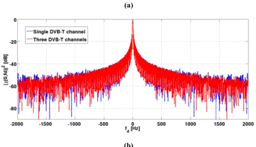
(2.11) First of all, three adjacent DVB-T channels (Figure 2.10) have been simulated through a Simulink® model, then analysed and processed to obtain the AF of the DVB-T multichannel waveform.

Figure 2.10 Multichannel DVB-T Spectrum

Multichannel DVB-T AF has the same shape of the single DVB-T AF as shown in Figure 2.11. Unwanted deterministic peaks in the AF are due to the known structure of the DVB-T signal, which includes pilots and guard intervals.

2 d f  B





1 1 2 2 * 2 0 0 ( , ) c ( ) ( ) d c , N N j f t j p f j p f d p p p d p p f e   s t s t e  dt e  AF f             



_

_ _  





,



p d AF  f





1 2







_

_



0 sinc | ( , ) | , , sinc c N c j p f d d d c p N f f AF f e AF f N f               



(44)

Figure 2.11 Single and Multichannel DVB-T Ambiguity Function

Specifically the single DVB-T channel ambiguity function is the envelope of multichannel DVB-T AF as confirmed by eq.(2.11) and the range resolution is

improved a factor of respect to the single DVB-T channel usage as shown in Figure

2.12. The side lobes present in the multichannel DVB-T AF due to the guard band between adjacent channels can be reduced by using windowing (Hamming, Kaiser, etc.).

Figure 2.12 Single and Multichannel DVB-T Ambiguity Function (Zoom View)

C

(45)

2.5. R

EAL DATA AMBIGUITY FUNCTIONS

As a preliminary step, three adjacent DVB-T channels have been acquired through a SDR (Software Defined Radio) board, then analysed and processed to obtain the AF of the DVB-T multichannel waveform. The central frequency is 754 MHz and the whole analysed signal shows about 24 MHz of bandwidth Figure 2.13.

Figure 2.13 Multichannel DVB-T Spectrum: real data

Once again, the ambiguity function have been computed and compared with the one obtained for a single DVB-T channel. Plots of the ambiguity function along time delay (range) and Doppler frequency are represented in Figure 2.14. It is worth noting that the

range resolution is improved by times with respect to the single DVB-T channel,

while the Doppler profile maintained the same behaviour. c

(46)

(a)

(b)

Figure 2.14 Multichannel AF from real data: a) Range profile: b) Doppler profile

The comparison between simulated and real data acquired with a low cost SDR architecture confirms the reliability of the DVB-T simulator.

(47)

Chapter 3. P

ASSIVE

R

ADAR

S

IGNAL

P

ROCESSING WITH

DVB-T S

IGNAL

3.1. S

INGLE

DVB-T C

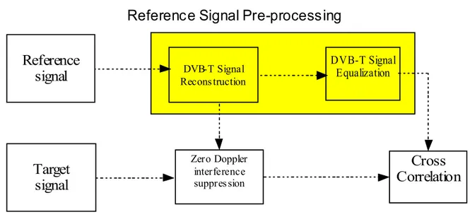
HANNEL 3.1.1. DVB-T Pre-processing

The goal of this system is to filter the reference signal in order to resolve two problems:  The multipath on the reference signal which can deteriorate the detection

performance;

 Mitigate the effects of pilot carriers and guard interval on the ambiguity function of the signal.

For this reason this system can be divided in to two sub-system as reported in Figure 3.1

Figure 3.1 Reference Signal Pre-processing block

Zero Doppler interference suppres sion

Reference

signal

Cross

Correlation

DVB-T Signal Equalization DVB-T Signal Recons truction

Reference Signal Pre-processing

Target

signal

(48)

3.1.1.1. DVB-T Signal Reconstruction

In the reference channel, except for the presence of the thermal noise, the main degradation is due to the presence of multipath. When digital transmissions are exploited by a PBR, the multipath removal from the reference signal can be performed by demodulating the signal received at the reference antenna. A copy of the transmitted signal can be obtained by re-modulating the resulting symbol sequence according to the standard transmission [20].

A general block diagram of a DVB-T receiver is presented in Figure 4.21. The previous stages of Front End and Analog to Digital Converter (ADC) have not been represented.

Figure 3.2 General block diagram of a DVB-T receiver

 Pre-FFT synchronization: it represents a first coarse approach in the estimation of the carrier frequency offset and the timing shift. It estimates the time offset and the fractional carrier frequency offset, using the time domain signal by applying the autocorrelation to the Guard Interval (GI). At its output, the GI can be removed, before calculating the FFT.

 GI removal: the GI inserted at the beginning of every OFDM symbol is removed.

 FFT: the Fast Fourier Transform is applied.

 Post-FFT synchronization: it is based on two different stages. The first one is an acquisition stage, where the integer carrier frequency offset is estimated, and the second one is a tracking stage consisting of the estimation of the residual carrier frequency offset and the sampling frequency offset.

The correct location of each carrier within the received OFDM symbol can be determined. The received signal in frequency domain can thus be represented as

(3.1)

 

1

 

2 0 , 0,1, 2,... 1 j kn N N n Y k y n e n N     



 

(49)

where denotes the channel transfer function of the channel and noise contribution.

Extracting the pilot carrier contribution from the signal, the transfer function of

the pilots is determined by

(3.2)

where denotes the well known pilot carrier

modulation in symbol .

The channel characteristics for the remaining carriers can now be obtained with linear extrapolation. This algorithm uses the transfer functions from two successive pilot

carriers and to determine the channel response for the data carriers in

between.

Let be the number of carriers between two pilots then the transfer function is given

by

(3.3)

where .

After the transfer function estimation, the information of the channel is used in order to equalize the OFDM symbol. In OFDM the equalization is simpler than traditional modulation because the information is carried within the frequency domain so that the equalization is only a subcarrier-wise multiplication by the equalization function. As with traditional systems two possible approach are presented: Zero-Forcing (ZF) and MMSE.

ZF approach in frequency domain simply tries to invert the channel. The equalization

function is given by:

(3.4)

 

H k W k

 

p Y K

   

_{ }

, ˆ , , 1, 2,..., , p p p p p Y l k H l k k N X l k  

 

, _p X l k l p k k_p 1 k_d d L

 

ˆ

 



ˆ



₁

  

ˆ



p p p d d H k H k H k H k L     0 d L_d

 

, Q l k

 

, 1 0,1, 2,... 1 Q l k  k  N

(50)

(3.5) With this equalization strategy, continual and scattered pilots are perfectly recovered in the equalized symbol and represents the milestones for the whole equalization[22]. ZF approach is the simplest way to equalize the signal but has some drawbacks. The most important one is the noise-enhancement. In fact, if the estimated value of the channel is low, when the channel inversion is imposed, the thermal noise can be enhanced. This effect can be shown by:

(3.6)

where the term can reach high values and affects the correct

de-mapping of the information .

In order to avoid this it is possibile to apply the MMSE approach which aims to find a

function which minimizes the mean square error given by:

(3.7)

The function can be written as:

(3.8)

where is substituted by and by which is the estimate noise

power at the receiver.

MMSE equalization eliminates the noise-enhancement because the perfomance of the

equalizer depends on the value of . If is big, the first term prevails at

the dominator and the equalizer acts as a ZF equalizer. If is small the second

term prevails and this prevents the noise-enhancement. The drawback of this method is the need to estimate the noise power at the receiver.

 

,

   

, ,

   

,

_{ }

, 0,1, 2,... -1 ˆ , X l k H l k Z l k Y l k Q l k k N H l k     

 

   

 

, , , , _ˆ , _ˆ _ˆ 0,1, 2,... 1 , , , Y l k H l k W l k Z l k X l k k N H l k H l k H l k      

   

_, ˆ _, W l k H l k

 

, X l k

 

, Q l k

 



2





   

 

2



, , , , , MSE E Z l k X l k E Y l k Q l k X l k

 

, Q l k

 



 



 

_{ }

 





2 ₂ 2 ( , ) ˆ , ₁ , arg min ˆ ˆ _, _ˆ _{ˆ ,} ˆ , Q l k _w w conj H l k Q l k MSE H l k _{H l k} conj H l k       _

 

, H l k H l kˆ ,

 

2 w  _ˆ2 w 

 

ˆ , H l k H l kˆ ,

 

ˆ , H l k

(51)

3.1.1.2. DVB-T Signal Equalization

The specific structure of the DVB-T signal (par. 2.3 ), and specifically the presence of guard interval and pilot tones, introduces a number of undesired deterministic peaks in the AF which might yield significant masking effect on the useful signal and produces false alarm.

The technique proposed here exploits a filtering based on Least Squares (LS) method described in par. 3.1.2.

The goal of this technique is to find a vector of tap weights which minimize the sum of squared errors:

(3.9)

where is the tap weight vector and is defined as follows:

(3.10)

and represents the position delay-Doppler of the k-th ambiguity.

Solving eq.(3.9) we obtain:

(3.11)

The matrix projects signal composed by samples in the subspace orthogonal

to the interference subspace defined by :

where is define as:

2 1 0 N w w i min E( w ) min  e( i )  



w e i

 

1 2 0 k M j f i * ref k ref k k e( i ) S ( i )  w S ( i  )e    



 k  f_k





1 * FILT H H

ref ref N ref ref

S S Zw _I Z Z Z  Z _S PS   P S_ref N



N



Z  P P

(52)

(3.12)

where represents positive range bin ambiguities and the number of positive

ambiguities.

Instead is defined as:

(3.13)

where  represents negative range bin ambiguities and_kn N . the number of negative_kn

ambiguities.

For the purpose of our analysis, the reference and surveillance antennas are assumed to be co-located with the reference antenna steered toward the transmitter and the surveillance antenna pointed in the direction to be surveyed.

The complex envelope of the signal at the reference channel is:

 

( ) ( )

ref T T

S t S t W t (3.14)

where S t is the complex envelope of the transmitted signal and_T

 

W t is the thermal_T( ) noise contribution. The complex envelope of the target signal in the surveillance

 

1 1 2 1 2 2 0 ... 0 0 ... . 1 e ... . 2 e j f ref j f ref S S P   

 

1

 

2 1 2 2 2 3 ... 1 e 3 e ... 2 e . ... . . ... . p p j f ref j f j f ref ref S S S   





2 1





2 1, 2... 2 e ... e p kp j f N j f N ref ref kp p N S N  S N                 _            _ _    kp  Nkp N

 





 





1 1 2 2 2 2 2 3 2 e ... e 3 e ... 1 e . ... . . . k kn k kn j f j f ref ref kn j f j f ref ref kn S S S S N              

 

1 2 2 .. . . ... e e ... . 0 ... . 0 k j f N ref j f N ref S N S N   1,.... ... 0 kn k N                             

(53)

 





j2 f tD _{( )}

Surv T Surv

S t S t e  W t (3.15)

The detection process in passive radar is based on the evaluation of the delay-Doppler cross-correlation function between the surveillance and the reference signal:





int * 2

0

, ( ) ( ) D

T

j f t

ref surv D ref surv

s s AF  f 



s t s t e  dt (3.16)

The reference signal after the equalization become:





1





2 1 2 2 2 * * 1 2 ˆ ˆ ( ) FILT j f t j f t

ref ref ref amb ref amb

S S t w S t e  w S t e  (3.17)

substituting eq. (3.15) into eq. (3.17) we obtain:

 

















1 1 1 1 2 2 2 2 2 2 * * 1 1 2 2 * * 2 2 ˆ ˆ ( ) ... ˆ ˆ ... FILT j f t j f t

ref T T T amb T amb

j f t j f t T amb T amb S S t W t w S t e w W t e w S t e w W t e                   (3.18)

It is worth noting that the number of ambiguities (in this case two) may vary according to the type of IO.

The 2D-CCF evaluated at the output of the equalization filter therefore becomes:

 





 





 









 













 

1 1 1 1 1 1 1 2 2 2 * * 1 1 1 2 2 2 * * 1 1 * 2 , ... ˆ ˆ ... , ... ˆ ˆ ... ... ˆ D FILT D j f t

ref Surv D T Surv T T

j f t

T Surv amb D T amb Surv

j f t j f t j f t

T amb T T amb Surv

amb S S t AF f S t W W t S t e W t W t w AF f f w S t e W t w W t e S t e w W t e W t w AF                                       











 













 

2 2 2 2 2 2 2 * 2 1 2 2 2 * * 2 2 ˆ , ... ˆ ˆ ... D j f t D T amb Surv j f t j f t j f t

T amb T T amb Surv

f f w S t e W t w W t e S t e w W t e W t                    (3.19)

If we merge the noise components we obtain:

 













 

1 2 * 1 1 * 2 2 ˆ , , ... ˆ ... , FILT

ref Surv D amb D

amb D S S t AF f w AF f f w AF f f N t               (3.20)

We can observe three components, the ambiguity function centered around the target delay and two contributions which cancel the ambiguities (in this case two) due to the target.

Feasibility study and development of a full digital passive radar demonstrator

UNIVERSITÀ DI PISA

Scuola di dottorato in Ingegneria “Leonardo da Vinci”

Corso di Dottorato di Ricerca in

TELERILEVAMENTO

Tesi di Dottorato di Ricerca