The ALMA Spectroscopic Survey in the HUDF: Constraining Cumulative CO Emission at 1 ≲ z ≲ 4 with Power Spectrum Analysis of ASPECS LP Data from 84 to 115 GHz

2020-11-27T15:06:22Z

Acceptance in OA@INAF

The ALMA Spectroscopic Survey in the HUDF: Constraining Cumulative CO

þÿEmission at 1 "r z "r 4 with Power Spectrum Analysis of ASPECS LP Data from 84

to 115 GHz

Title

Uzgil, Bade D.; Carilli, Chris; Lidz, Adam; Walter, Fabian; Thyagarajan,

Nithyanandan; et al.

Authors

10.3847/1538-4357/ab517f

DOI

http://hdl.handle.net/20.500.12386/28587

Handle

THE ASTROPHYSICAL JOURNAL

Journal

887

The ALMA Spectroscopic Survey in the HUDF: Constraining Cumulative CO Emission

at 1

 z  4 with Power Spectrum Analysis of ASPECS LP Data from 84 to 115 GHz

Bade D. Uzgil1,2 , Chris Carilli1,3 , Adam Lidz4 , Fabian Walter1,2 , Nithyanandan Thyagarajan1 , Roberto Decarli5 , Manuel Aravena6 , Frank Bertoldi7 , Paulo C. Cortes8,9 , Jorge González-López6,10, Hanae Inami11,12, Gergö Popping2 ,

Dominik A. Riechers13,14,18 , Paul Van der Werf15, Jeff Wagg16, and Axel Weiss17

1

National Radio Astronomy Observatory, Pete V. Domenici Array Science Center, P.O. Box 0, Socorro, NM 87801, USA;buzgil@nrao.edu

2

Max-Planck-Institut für Astronomie, Königstuhl 17, D-69117, Heidelberg, Germany 3

Cavendish Laboratory, University of Cambridge, 19 J J Thomson Avenue, Cambridge CB3 0HE, UK 4

Department of Physics & Astronomy, University of Pennsylvania, 209 South 33rd Street, Philadelphia, PA 19104, USA 5

INAF–Osservatorio di Astrofisica e Scienza dello Spazio, via Gobetti 93/3, I-40129, Bologna, Italy 6

Núcleo de Astronomía de la Facultad de Ingeniería y Ciencias, Universidad Diego Portales, Av. Ejército Libertador 441, Santiago, Chile 7

Argelander-Institut für Astronomie, Universität Bonn, Auf dem Hügel 71, D-53121 Bonn, Germany 8

Joint ALMA Observatory—ESO, Av. Alonso de Córdova, 3104, Santiago, Chile 9

National Radio Astronomy Observatory, 520 Edgemont Road, Charlottesville, VA 22903, USA

10_{Instituto de Astrofísica, Facultad de Física, Pontificia Universidad Católica de Chile, Av. Vicuña Mackenna 4860, 782-0436 Macul, Santiago, Chile} 11

Univ. Lyon 1, ENS de Lyon, CNRS, Centre de Recherche Astrophysique de Lyon(CRAL) UMR5574, F-69230 Saint-Genis-Laval, France 12_{Hiroshima Astrophysical Science Center, Hiroshima University, 1-3-1 Kagamiyama, Higashi-Hiroshima, Hiroshima 739-8526, Japan}

13

Department of Astronomy, Cornell University, Space Sciences Building, Ithaca, NY 14853, USA 14

Max-Planck-Institut für Astronomie, Königstuhl 17, D-69117 Heidelberg, Germany 15

Instituto de Astrofísica, Facultad de Física, Pontificia Universidad Católica de Chile, Av. Vicuña Mackenna 4860, 782-0436 Macul, Santiago, Chile 16

SKA Organization, Lower Withington Macclesfield, Cheshire SK11 9DL, UK 17

Max-Planck-Institut für Radioastronomie, Auf dem Hügel 71, D-53121 Bonn, Germany Received 2019 July 29; revised 2019 October 18; accepted 2019 October 25; published 2019 December 9

Abstract

We present a power spectrum analysis of the ALMA Spectroscopic Survey Large Program (ASPECS LP) data from 84 to 115GHz. These data predominantly probe small-scale fluctuations (k = 10–100 h Mpc−1) in the aggregate CO emission in galaxies at 1 z  4. We place an integral constraint on CO luminosity functions (LFs) in this redshift range via a direct measurement of their second moments in the three-dimensional(3D) autopower spectrum,finding a total CO shot-noise power PCO,CO(kCO 2 1( - ))1.9´102 μK2(Mpc h−1)3. This upper limit (3σ) is consistent with the observed ASPECS CO LFs in Decarli et al. but rules out a large space in the range of

( ( - ))

PCO,CO kCO 2 1 inferred from these LFs, which we attribute primarily to large uncertainties in the normalization Φ_*and knee L_*of the Schechter-form CO LFs at z>2. Also, through power spectrum analyses of ASPECS LP data with 415 positions from galaxies with available optical spectroscopic redshifts, wefind that contributions to the observed mean CO intensity and shot-noise power of MUSE galaxies are largely accounted for by ASPECS blind detections. Finally, we sum thefluxes from individual blind CO detections to yield a lower limit on the mean CO surface brightness at 99GHz of áTCOñ =0.550.02μK, which we estimate represents 68%–80% of the total CO surface brightness at this frequency.

Unified Astronomy Thesaurus concepts: High-redshift galaxies(734);Molecular gas(1073)

1. Introduction

The formation of molecular clouds from atomic hydrogen gas and their subsequent consumption as fuel for star formation are important transitions linking the early stages in the life cycle of the interstellar medium (ISM) to the evolution of galaxies. Obtaining an unbiased and complete measure of the cold gas content and star formation activity of galaxies as functions of cosmic time provides insight into the underlying physical processes that regulate this evolution. With the cosmic star formation rate density (SFRD) well characterized out to z∼3–4 and rest-frame UV observations setting constraints on the SFRD into the first billion years after the Big Bang (see, e.g., Madau & Dickinson2014for a review), there are ongoing efforts to complement this understanding with concurrent trends in the atomic (HI; e.g., Neeleman et al. 2016) and

molecular(H2; e.g., Decarli et al.2019) gas history, particularly

during the epoch of galaxy mass assembly at z∼2, when cosmic star formation activity was approximately 10 times

higher than in the present epoch and more than half of the stellar mass in the universe was accumulated (Madau & Dickinson2014).

While the cosmic HI gas density has been inferred from observations of damped Lyα systems in quasar spectra at z5 (Wolfe et al.2005), a more direct method is to observe the HI gas in emission via the 21cm hyperfine transition. The 21cm experiments have constrained the atomic gas density in cosmic volumes out to z∼0.8 (Chang et al.2010; Switzer et al.2013),

and extended surveys are underway (e.g., CHIME, Tianlai, HIRAX, BINGO, and the Ooty Wide Field Array) to push this redshift limit in a continuous range out to z∼3.5. As the primary science goal of many of these experiments is to use HI as a tracer of large-scale structure in order to measure the imprint of baryon acoustic oscillations, these experiments utilize an observational technique known as line intensity mapping to survey large areas of sky ( ( 103_–104_deg2_{)) with}

coarse angular resolution ( ( 10 arcmin)) in a spectral line across a wide fractional bandwidth (30%–60%), resulting in 3D maps of spatially confused line emission throughout

© 2019. The American Astronomical Society. All rights reserved.

18

cosmological volumes. Line intensity mapping experiments measure the surface brightness fluctuations in the targeted spectral line, as well as any additional line or continuum emission contributing to the aggregate surface brightness at the observed frequencies, via the power spectrum.

Owing to the large collecting areas and wide bandwidths available in existing facilities such as the Atacama Large Millimeter Array(ALMA), Karl G. Jansky Very Large Array (JVLA), and IRAM NOrthern Extended Millimeter Array (NOEMA), the cosmic evolution of molecular gas density has already been measured out to z∼4—well into the epochs of galaxy mass assembly and peak cosmic star formation history —with various surveys targeting different rotational J transi-tions of the CO molecule as an H2 gas tracer (Walter et al.

2014, 2016; Pavesi et al. 2018). Unlike the HI intensity mapping experiments, the CO surveys performed blind spectral scans, or so-called molecular deep fields, to build a census of galaxies’ gas content by detecting emission from individual CO-emitting sources that are brighter than the survey’s flux limit. Given the relatively small fields of view and longer baselines of the telescopes employed in these efforts, the molecular deep fields are characterized by survey areas

(

 100–101_arcmin2_{)) and angular resolutions ( (}

)  100 _arcsec) well-suited for observing individual galaxies.

The ALMA Spectroscopic Survey Large Program(ASPECS LP) in the Hubble Ultra Deep Field (HUDF) is the latest example of a blind spectral scan that has resulted—with 68 hr of total telescope time to scan the full ALMA Band 3 from 84 to 115GHz—in the tightest blind constraints to date on the evolution of CO luminosity functions (LFs), which directly translate to measurements on the cosmic molecular gas density (Decarli et al. 2019, hereafter D19) over ∼12Gyr of the

universe’s history, revealing the levels of accumulation and consumption of molecular gas in galaxies from z∼4 to the present day. The ASPECS LP targeted an∼4.6arcmin2field in a region of the HUDF containing the deepest near-infrared (near-IR) photometric data on the sky (Illingworth et al.2013; Koekemoer et al.2013) and ∼1500 spectroscopic redshifts for

rest-frame optically/UV-selected galaxies (Inami et al. 2017),

which facilitated the confirmation and redshift identification of blindly detected line candidates and further enabled the characterization of physical properties such as molecular gas mass, stellar mass, active galactic nucleus (AGN) fraction, metallicity, IR luminosity, and star formation rate(SFR) for all secure detections in thefield, as well as for hundreds of fainter sources. Papers from the ASPECS team discuss key results from the ASPECS LP scan in ALMA Band 3, including the observed CO LFs (D19), which also contain a detailed

description of the ASPECS survey and ancillary data sets, blind searches for spectral line and continuum detections (González-López et al. 2019, hereafter GL19), MUSE-based

CO identifications and demographics of the ASPECS CO sample from spectral energy distribution (SED) modeling (Boogaard et al. 2019, hereafterB19), theoretical perspectives

on the cosmic molecular gas density evolution (Popping et al.

2019), ISM properties (Aravena et al. 2019), and stacking

analysis with MUSE galaxies in the UDF.

In this paper, we consider the ASPECS LP Band 3 data in the context of a power spectrum analysis. Although we adopt the power spectrum approach used in line intensity mapping experiments, our data set is inherently distinct from those produced by the aforementioned line intensity mapping

experiments, given the marked differences in sky coverage and angular resolution. Our overarching goals, however—to (1) probe the flux from galaxies below the survey’s sensitivity threshold for individual line detections and (2) improve the constraints on the observed cumulative emission(from CO, in our case) by measuring surface brightness fluctuations within the survey volume—are akin to the objectives common throughout the line intensity mapping experimental landscape (see, e.g., Kovetz et al. 2017, for a review), including experiments with goals of mapping the CO intensity field at 2<z<3 to determine the cosmic molecular gas density (Keating et al.2016; Li et al.2016). Furthermore, the parallel

analysis by the ASPECS team to extract individual CO detections, along with the rich multiwavelength data sets available in the HUDF, provide valuable information to aid in the interpretation of the power spectrum results and enable an exploration of the complementarities between the two approaches.

The organization of this work is as follows. In Section2, we place ASPECS in the context of a power spectrum analysis, identifying, e.g., the relevant scales that the survey covers in Fourier space. In Section 3, we describe the Band 3 data, as well as details regarding our approach to measuring the power spectrum. Our results on lower limits from blindly detected sources, the three-dimensional (3D) CO autopower spectrum, and statistical analysis of the CO fluctuation data including information from galaxy catalogs are presented in Section4. In Section5, we briefly discuss our findings in the framework of a comparison between the power spectrum analysis and the blind line search in recovering the true CO power and comment on the capability of current facilities to measure the CO power at high redshift. Finally, we summarize ourfindings in Section6. Throughout this work, we adopt a cosmological model with ΩM=0.7, ΩΛ=0.3, Ωk=0, and =h H0 100=0.70.

2. ASPECS in the Context of a Power Spectrum Analysis 2.1. Mapping Survey Dimensions from Real Space to Fourier

Space

The original goal of the ASPECS LP—to reach a sensitivity such that the predicted“knee” of the CO LF could be reached at z∼2″ (Walter et al.2016)—was a key driver of the chosen

survey parameters,19 including total observing time (and, hence, rms sensitivity per beam per channel), spectral resolutionΔνchn, survey bandwidthΔνBW, array configuration

(or synthesized beam size Δθb), and survey width ΔθS. We do

not—and, in some cases, cannot—alter these experimental parameters for the purposes of the power spectrum analysis, except when redefining Δνchn and ΔθS, to be explained in

more detail below. Upon adopting a target redshift for the observations,Δνchn,ΔνBW,Δθb, andΔθScan be translated to

physical comoving length scales via the standard cosmological relations, and, thus, set the range of distances where statistical correlations between galaxies can be probed. Given that 11 of the 16 secure, blindly detected sources in GL19 with known redshifts in ASPECS correspond to CO(2–1) emitters, we have adopted a target redshift zcen,CO(2-1)=1.315 to represent the

redshift of CO(2–1) emission observed at the band center, νcen=99.572 GHz. We discuss the issue of redshift

ambi-guities in the CO line emission in Section2.2.1.

19

See Walter et al.(2016) for more on the rationale behind the opted survey design.

2.1.1. Real-space Dimensions

The largest physical scale, then, accessible in real space in the line-of-sight dimension, r_P,max, is determined by the survey’s frequency coverage, ΔνBW,

( ) ( ) ( ) ( ) 

ò

whereχ(z) is the comoving line-of-sight distance to redshift z. In the above expression, zmin and zmax correspond to the

minimum and maximum redshifts observed at, respectively, the highest and lowest frequencies, νmax=114.750 GHz and

νmin=84.278 GHz, of the survey bandwidth, so that zmin=

( )

nrest,CO 2 1- nmax-1=1.009,zmax=nrest,CO 2 1( - ) nmin- =1 1.735, and rP,max=1054.8 Mpch−1.

Similarly, the channel resolution establishes the smallest physical scale probed in the line of sight, r_P,min:

( ) ( ) ( )

 =c + -c

r ,min zchn,i 1 zchn,i. 2

Here zchn,iandzchn,i+1correspond to redshifts of the ith and ith +1 channels at observed frequencies νiand ni+1=ni+ Dnchn, so thatzchn,i=nrest,CO 2 1( - ) ni-1andzchn,i+1=nrest,CO 2 1( - ) (ni+ Dnchn)- 1. BecauseΔνchnis a constant across the band,

the physical separation between channels increases gradually with redshift. In practice, then, to facilitate computing the Fourier transform, we do not use Equation(2) when converting

channel widths from frequency to physical distance. Rather, we define channel separations of equal width in space, dividing the total line-of-sight distance, r_P,max, by the number of channels, Nchn=196, in the band, yielding rP,min=5.38 Mpch−1. This

value is equal to the channel width at νcenand is a reasonable

substitute for the true r_P,min per channel, due to the modest 12.6% relative change in r_P,min from either band edge to the band center. Note that the choice of Nchn=196 reflects the fact

that we have imaged the ASPECS data cube while rebinning the native ALMA channel resolution by a factor of 40 (i.e.,

n n

D chn= D 40chn), compared to the factor of 2 rebinning ( nD chn= Dn2chn) used when imaging the data cube for purposes of CO line searches, etc. The coarser spectral resolution Δν40chn=0.156 GHz, with a velocity width

Dv40chn~470 kms−1atνcen, ensures that most CO emission

is spectrally unresolved throughout the data cube; the median FWHM of the Gaussian line flux profiles of the blindly detected lines in ASPECS is 355 km s−1, and the full range of observed FWHMs spans 40.0–617 km s−1 (GL19). We favor

the larger channel width to avoid significant contributions to the power spectrum from emission lines with FWHM? Δvchn,

since we do not attempt to characterize the effect of falsely elongating the observed flux density of these lines from the ∼kpc scales of localized emission within the CO-bright galaxy to∼Mpc scales when converting channel widths to cosmolo-gical line-of-sight distances.

In the transverse, or on-sky, dimensions, the largest and smallest physical scales accessible to probe COfluctuations in real space, r_⊥,max and r_⊥,min, are determined by the survey width and synthesized beam size,

( ( )) q ( )

= D

^

-r ,max DA,co zcen,CO 2 1 S, 3

( ( )) q ( )

= D

^

-r ,min DA,co zcen,CO 2 1 b, 4

where the units ofΔθSandΔθbare in radians, andDA,co( )z , the comoving angular diameter distance at redshift z, is equal to χ(z) for Ωk=0.

As the antenna primary beam size grows with observed wavelength,ΔθbandΔθSgradually increase with redshift across

the survey bandwidth. As with r,min, we adopt fixed values for each quantity calculated at νcen, where change is modest

to either band edge. At this frequency, the synthesized beam—an ellipse described by the FWHMs of its major and minor axes,Dqb,maj andDqb,min, respectively—for the full data set is

q q q

D = Db b,maj´ D b,min= 1. 80 ´ 1. 48 , corresponding to como-ving transverse distances 0.0250 Mpc h−1× 0.0205 Mpch−1. (For reference, D = qb 2. 11 ´ 1. 67 at νmin, and D =qb

 ´ 

1. 51 1. 32 at νmax.) Expressing the beam area as

( )

q q p

= D D

Ab b,maj b,min 4 ln 2, we letr^,min= Ab =0.0240

Mpch−1. Note that the data cube for an interferometric image is gridded with rectangular cell sizesΔθcella factor of a few times

smaller than Δθb, chosen such that Δθcell represents Nyquist

sampling of the longest-baseline visibility data (Taylor et al.

1999). Thus, the smallest transverse dimension present in the data

set is actuallyΔθcell=0 36 (=0.005 Mpc h−1at νcen), though

there is no information on CO fluctuations contained within physical scales smaller thanΔθb.

At νcen, the full width of the survey spans roughly

q

D S,tot= ¢2. 83at a primary beam response cutoff of 20%. The sensitivity profile of the mosaic primary beam implies, however, that the antenna response drops to 50% at DqS,HPBW» ¢2. 15. Beyond this threshold, the rms noise statistics deteriorate rapidly, as indicated by the noise map20in Figure1 forνcen. Not only is

the overall rms noise higher for the surveyfield past the half-power point of the mosaic primary beam, the spatial variation of the rms is also significantly greater in this region, compared to the central∼4arcmin2, e.g., where the rms remains mostly between 0.13 and 0.18 mJy beam−1 channel−1, gradually reaching 0.3 mJy beam−1 channel−1at the half-power point;21 beyond the half-power point, the rms increases from 0.3 to 0.8 mJy beam−1 at the outermost edge of the mosaic, defined by the primary beam cutoff at 20% antenna response. We note as well that results from the blind search for individual CO emitters in ASPECS data(GL19) suggest a lower fidelity (i.e.,

higher probability of false identification) of line candidates in the survey volume corresponding to<50% antenna response, so other studies(e.g., CO LF measurements presented inD19)

within the ASPECS collaboration have excluded data that lie outside DqS,HPBW. Thus, we limit our analysis to a square

region (shown as the black dotted square in Figure 1) with

area Dq2S =(1.84 arcmin)2 =(1.53 Mpch-1 2), chosen to lie within the 50% power threshold at all observed frequencies. For reference, this region encompasses roughly 85% of the volume contained within DqS,HPBW and 55% of the volume

withinDqS,tot.

2.1.2. Fourier-space Dimensions

Since we will be characterizing the COfluctuation field by its power spectrum, we must relate the relevant physical scales probed in real space (Equations (1)–(4)) to the wavevectors

20

Noise maps were generated by calculating the rms, in units of mJybeam−1, for each pixel, using all surrounding data within a 70pixel×70pixel box. 21

Here the quoted rms values refer to channel widths withΔνchn=Δν2chn, or

with magnitudek= k2+k^2 that are accessible to ASPECS in Fourier space: ( )   p p = ^ = ^ k r k r 2 and 2 , 5 ,min ,max ,min ,max ( )   p p = ^ = ^ k r k r 2 2 and 2 2 , 6 ,max ,min ,max ,min

where k_P,minand k_⊥,minrepresent the lowest k modes available in the line-of-sight and transverse dimensions, respectively; note that these fundamental modes map to the largest scales accessible in real space, with frequencies spanning a single oscillation acrossΔνBWandΔθS. The highest k modes probed

by the survey, k_P,max and k_⊥,max, correspond to Nyquist frequencies, k,Nyqµ1 2( r,min) and k^,Nyqµ1 2( r^,min), mapping these modes to the smallest physical scales in the survey.

Table1summarizes the ASPECS survey parameters adopted for the power spectrum analysis and their mappings to physical dimensions in real and k space. In Figure 2, we indicate the location of k_P and k_⊥ values for ASPECS relative to the predicted total CO(2–1) power—including both clustering and shot-noise contributions—at z=1 from Sun et al. (2018). The

ranges of transverse and line-of-sight k modes have important

implications to be considered when computing the power spectrum.

For example, the large bandwidth and relatively narrow survey area of ASPECS dictate that the CO brightness fluctuations on physical scales larger than the survey width,

= ^

r ,max 1.53Mpch−1(i.e., for <k k^,min=4.107hMpc−1), will be probed exclusively by k_P modes. Thus, the power spectrum measured at k<4.107 hMpc−1will be an inherently one-dimensional(1D) measurement, dominated by power from the shorter wavelength, high-k_⊥modes projected into the line of sight. These physical scales are important, however, for extracting information about large-scale clustering. Based on models(e.g., Pullen et al. 2013; Sun et al.2018) for the total

Figure 1.Noise maps atνmin=84.3 and 91.9GHz, νcen=99.6 and 107.3GHz, and νmax=114.8 GHz. Solid contours indicate curves of constant rms noise (in

units of mJy beam−1). Notable changes in the respective rms at different frequencies are due to an overlap of the frequency bands in the observations (top right panel) and decreasing atmospheric transmission at higher frequencies(bottom row;GL19). The black and red dashed contours show, respectively, the mosaic primary beam

Table 1

Mapping ASPECS Survey Parameters to Real- and Fourier-space Dimensions Survey bandwidth,ΔνBW 84.278–114.750GHz

Channel resolution,Δνchn 0.156GHz

Survey width,ΔθS 1 84

Beam size,Δθb 1 80×1 48

Central redshift,zcen,CO 2(-1) 1.315     r,min r r,max 5.38 Mpch-1<r<1054.8Mpch−1 ^  ^ ^ r,min r r,max 0.0240 Mpch-1<r^<1.53_Mpch−1     k,min k k,max 0.00596hMpc-1<k<0.584_hMpc−1 ^  ^ ^ k,min k k,max 4.107hMpc <-1 k^<130.900_hMpc−1

CO power spectrum at the redshift range relevant to this study, we expect any power from galaxy clustering between dark matter halos, PCO,CO(k z, )

clust _{, to dominate the total CO power}

spectrum, PCO,COtot (k z, ), up to k  1 hMpc−1 compared to contributions from small-scale clustering of galaxies that share a common host dark matter halo or shot-noise power, PCO,COshot (see Figure2). If the CO surface brightness fluctuations, áTCOñ, trace the large-scale clustering of galaxies with some mean bias factor, ábCOñ, that offsets CO-emitting galaxies from the underlying dark matter distribution, i.e., if

( )= á ( )ñ á ( )ñ ( ) ( )

PCO,CO k T z b z P k z, , 7

clust

CO 2 CO 2 m,m

where Pm,m(k z, ) is the linear matter power spectrum (appro-priate for k< 0.1 h Mpc−1), then the low-k component of the power spectrum is, in principle, useful for constraining the aggregate CO emission within a given cosmological volume. Note that the units of PCO,CO(k z, )

clust in Equation (7) are in μK2_{(Mpc h}−1₎3_for ( ) áTCO z ñinμK, Pm,m(k z, )in(Mpc h−1)3, and a dimensionlessbCO( )z .

For physical scales smaller than r^,max=1.53 Mpch−1 (i.e., for kk^,min=4.107 hMpc−1), it is clear from Table 1 that k can have contributions from both k_⊥ and k_P as long as k= k2+k^2 is within the range k= 4.107–130.900hMpc−1—we are measuring a full 3D power spectrum in this regime—though the k_⊥ modes, with wavelengths on the order of Δθb up to ΔθS, provide most

of the information on the power at these scales. At z∼1, we expect any power from galaxy–galaxy clustering at k4 hMpc−1 to be buried under a Poissonian shot-noise component,P_CO,COshot ( )k, dominated by bright CO emitters in the survey volume. By restricting our analysis to k10 h Mpc−1, where the true power spectrum is expected to beflat, the power spectrum measurement is unaffected by the highly anisotropic ASPECS survey window function.

2.2. Inherent Challenges to the Autopower Spectrum Measurement

One of the intrinsic benefits of the autopower spectrum measurement is its sensitivity to intensityfluctuations from all sources, faint and bright, contained within the survey volume. The inclusion in the power spectrum analysis of all flux densities present in the data cube also presents specific challenges to the interpretation of the measured power. For the purpose of the ASPECS power spectrum analysis, a primary concern is the redshift ambiguity of CO emission within the observed survey bandwidth. We also briefly discuss the effects of a possible contribution from continuum emission.

2.2.1. Redshift Ambiguity of CO Emission

As with blindly detected individual line candidates, where the redshift of a line candidate without spectroscopically or photometrically confirmed counterparts can be ambiguous, the true redshifts of sources contributing to the intensity fluctuations contained within the ASPECS survey volume are unknown. However, in defining a real- and Fourier-space grid to perform our power spectrum calculations, we have assumed a specific target redshiftzcen,CO 2 1( - )=1.315—corresponding to the central redshift of CO(2–1) in the ASPECS bandwidth —for the emission. While CO(2–1) is expected to dominate the mean surface brightness at 99GHz, based on the number of blind detections in ASPECS relative to other line transitions, for example, it is not the only source of spectral line emission present in the survey volume. Figure 2 ofD19

illustrates the number of different spectral lines that are, in principle, observable within the ASPECS frequency coverage, emitted from galaxies within the local universe (such as CO(1–0) at z<0.37) and at high redshift (such as any CO transition from J> 2 at z > 2). Thus, the measured autopower spectrum of the ASPECS data should be interpreted as a sum of the power from surface brightness fluctuations from all relevant CO transitions, ( ) ( ) ( ) ( ) ( ) ( ) ( ) ( ) ( ) ( ) ( ) ( ) ( ) ( ) ( ) ( ) ( ) ( ) = + + + + - - -- - -- - -- - -P k P k P k P k P k ..., 8 CO,CO CO 1 0 ,CO 1 0 CO 1 0 CO 2 1 ,CO 2 1 CO 2 1 CO 3 2 ,CO 3 2 CO 3 2 CO 4 3 ,CO 4 3 CO 4 3

where we truncate the sum, in practice, to include contributions from CO(1–0), CO(2–1), CO(3–2), and CO(4–3), because the ASPECS survey has only resulted in CO blind detections up to J=4 (GL19). Each term in the right-hand side of the

above equation is expressed as a function of wavenumber ( - -( ))

kCOJ J 1 , corresponding to the Fourier space defined at the emitted redshift of the respective J transition at the band center. For reference, at νcen=99.572 GHz, CO(1–0), CO(3–2), and

CO(4–3) can be emitted from z=0.157, 2.470, and 3.629, respectively. The k appearing on the left-hand side of Equation(8) is intentionally ambiguous; ultimately, we would

like to write PCO,CO( )k as PCO,CO(kCO 2 1( - )). We can convert ( - -( ))

kCOJ J 1 to kCO(2-1), defined atzcen,CO 2 1( - ), using so-called

Figure 2.Total predicted CO(2–1) power from Sun et al. (2018). Here CW13 and G14 refer to different prescriptions used for relating CO luminosities to estimated IR luminosities in the model, based on the compilations in Carilli & Walter(2013) and Greve et al. (2014). Power from clustering and shot noise dominates at k<1 and k>1 h Mpc−1, respectively. Vertical dashed lines indicate k values corresponding to ASPECS survey parameters, namely, survey bandwidth ΔνBW, channel width, survey widthΔθS (1 84), antenna

primary beam (0 98), mosaic spacing (25 4), and synthesized beam size Δθb(1 8 × 1 5).

“distortion” factors (as given in, e.g., Lidz & Taylor 2016), ( ) ( ) ( ) ( ) ( ( )) ( ) ( ( )) ( ( )) ( ) a = = ^ - - ^ -^ -z k k D z D z 9 J J J J J J cen,CO 1 ,CO 2 1 ,CO 1 A,co cen,CO 1 A,co cen,CO 2 1 and ( ) ( ) ( ) ( ) ( ) ( ) ( ( )) ( ) ( ( )) ( ) ( ( )) ( ( )) ( )    a = = ´ + + - - -z k k H z H z z z 1 1 , 10 J J J J J J J J cen,CO 1 ,CO 2 1 ,CO 1 cen,CO 2 1 cen,CO 1 cen,CO 1 cen,CO 2 1

that relate transverse and line-of-sight comoving distances, respectively, between the true emitted redshift of intensity fluctuations, zcen,CO(J- -(J 1)), and the adopted redshift

( - )

zcen,CO 2 1. In Equation (10), the expression H(z) refers to the Hubble parameter at redshift z. Finally, combining Equations(8)–(10), we obtain the total CO power in terms of

k_CO(2-1): ⎡ ⎣ ⎢ ⎛ ⎝ ⎜ ⎞ ⎠ ⎟⎤ ⎦ ⎥ ⎥ ( ) ( ) ( ) ( ) ( ) ( ) ( ) ( ) ( ) ( ) ( ) ( ( )) ( ( )) ( ( )) ( ( )) ( ) ( ( )) ( ) ( ( ))   

å

The multiplicative pre-factor1 (a a^2 ) in the second term on the right-hand side of the above equation represents the ratio of volume probed by the survey in CO(2–1) relative to the other J transitions. The ratio 1 (a a >^2 ) 1 for J=1, reflecting the fact that the volume probed by CO(1–0) is less than the volume probed by CO(2–1), while the opposite is true for the J=3 and 4 transitions, where

 <

a a^ 1 1

2 . Contributions to the total measured power from different CO transitions are correspond-ingly magnified or demagnified when projected into the CO(2–1) frame (Equation (11)).

Note that Equation(11) is only valid for large separations in

redshift between the sources of CO emission; if there is overlap between the redshift ranges of the different transitions in the ASPECS survey volume, then Equation(11) will contain

cross-terms that represent the cross-power spectrum between the CO transitions that overlap in redshift. For the ASPECS spectral coverage, we point out that there is a small overlap in redshift for the CO(3–2) and CO(4–3) in the survey at z=3.011–3.107 (see Table 1 inD19), but the cross-terms here will be negligible

given that the mean redshifts zcen,CO 3 2( - )=2.470 and ( - )=

zcen,CO 4 3 3.629are widely separated. 2.2.2. Continuum Emission

A search for continuum emission in the ASPECS LP Band 3 data was presented in GL19. This study identified six

continuum sources, with the brightest emission on the order of ∼10μJy, indicating that the continuum level in each channel of the 3 mm cube is negligible for our purposes. To ensure, however, that our power spectrum measurements reflect power from spectral line (CO) fluctuations only and do not contain contributions from the continuum, we perform continuum subtraction on the cube with a linear baselinefit, described in Section3. This continuum-subtracted cube is used for all power spectrum and cross-power spectrum analyses.

3. Data and Methods

The ASPECS LP survey consisted of two blind frequency scans at 1.2 and 3 mm in the HUDF(Beckwith et al.2006). The

methods and subsequent power spectrum analysis presented here utilize the 3 mm observations, which consist of a 17-pointing mosaic over∼4.7arcmin2 atfive frequency tunings spanning the full extent of ALMA Band 3. As described inD19

(see their Section 2.2 for more details) of this series, the resulting visibility data were imaged using the CASA task tclean—with natural weighting applied in the uv-plane and frequency rebinning over two of the native 3.91 MHz spectral resolution elements—to produce an image cube with mean rms=ásN,2chnñ =1.96´10-4Jybeam−1channel−1across all 3935 channels in the cube. Here the rms per channel of the data cube has been inferred by computing the rms in the central 70× 70 pixels for each channel map; given the lack of known sources in this 70 × 70 pixel wide skewer through the data cube, the rms in this region is expected to be a valid representation of the noise in the cube. (Recall that Figure 1

shows the spatial variation of the rms noise at a number of representative frequencies.) At νcen, for example, this mean rms

translates to a mean surface brightness sensitivity in units of Jysr−1 and, via the Rayleigh–Jeans law, a mean brightness temperature sá N,2chnñ =2.76´106Jysr−1=9.07×103μK. In the context of a power spectrum analysis, this mean rms can give rise to a spectrally featureless(i.e., “white”) noise power, PN,

( ) s

= á ñ

PN N ,2chn 2Vvox,2chn, 12 where Vvox,2chn refers to the voxel volume defined by

the beam area and channel width. At zcen, Vvox,2chn=

( ) ( ) q n D D = _{0.024 Mpc h}- ´ _{0.27 Mpc h}- =_{1.57 10}´ -b 2 2chn 1 2 1 4 (Mpc h−1₎3 _{and implies P} N=1.29×104 μK2(Mpc h−1)3.

This image cube, referred to in this work as T0,2chn, has served as the principal data product exploited in a variety of analysis efforts by the ASPECS team, including the identification of blindly detected individual line emitters. The catalog of reliable blind detections—specifically, where the probability that the line is due to noise has been determined inGL19to be less than 10%—is reproduced in Table 2.

As already discussed in Section2.1.1, the 7.81 MHz channel width is toofine a spectral resolution for the purposes of the power spectrum analysis. Thus, unless otherwise noted, we have imaged with a frequency rebinning over 40 native spectral resolution elements to obtain an image cube T0,40chn (or T0,

hereafter, for brevity) characterized by a lower mean rms, s

á ñ =_4.55´₁₀

-N,40chn 5Jybeam−1channel−1»ásN,2chnñ 20, as depicted in the bottom right panel of Figure3. Note that the noise power remains unchanged as the larger channel width counteracts the change in sá N,40chnñ2 (see Equation (12)).

After imaging and applying a primary beam correction to correct flux densities for the effect of the mosaic sensitivity pattern, we estimate and subtract any possible continuum emission by running CASA task imcontsub in the full cube to ensure that all surface brightnessfluctuations in T0are due to

spectral emission. The continuum was approximated using a linear baseline fit across all channels to prevent introducing artificial spectral structure. We inspected rms levels and spectra at random positions in the cube before and after continuum subtraction, finding negligible (less than 0.1%–1%) change in both quantities, confirming our expectations based on GL19

(see Section2.2.2).

For the purposes of the power spectrum analysis, however, we do not work directly with T0or T0,2chn. That is, we do not assess the level of astrophysical signal in the 3 mm data set by taking the (auto)power spectrum of T0,PT T0,0( )k , defined as

( ) ( ) ( p d) ( ) ( ) ( )

áT0*k T0 k¢ ñ º 2 3 D k- ¢k PT T0,0 k , 13

where (_{2p d})3 (_{k- ¢ =k})

_ò

D 3 is a Dirac delta

function. Explicitly, PT T0,0( )k is the 3D average of the Fourier transform of the two-point correlation function,

(∣ ∣) ( )

x x - ¢ =x x r :

_ò

from astrophysical signal at the target and/or other redshifts, as well as instrument noise, characterized by PN. In Sections2.2.1

and 2.2.2, we explained why the main astrophysical source of surface brightnessfluctuations in the data cube is expected to be the CO line transitions (from J=1, 2, 3, 4). As our estimated noise power is 2–3 orders of magnitude greater than the predicted CO power spectrum signal, the instrument noise introduces a significant bias in the measured power spectrum throughout all k probed by the survey. Thus, in this low signal-to-noise(S/N) regime, we seek a way to remove the noise bias from the data in order to accurately measure the CO signal; we

avoid subtracting this noise-bias term from the data based on independent estimates of PNthat may not reflect the true noise

amplitude in the data or exhibit deviations from Gaussianity that would, for example, invalidate Equation (12), which

assumes that the measured rms describes a white-noise randomfield.

Dillon et al. (2014) demonstrated that it is possible—and,

indeed, preferable when the expected S/N is subunity, as in the current generation of reionization-era 21cm intensity mapping experiments discussed in their paper—to remove the noise bias by computing the cross-power spectrum of two data cubes, e.g., TIand TII, that are derived as subsets of the original data cube,

T0, in a manner that preserves the real and Fourier spaces

sampled by T0. For ASPECS data, we can split the original

CASA measurement set22T0into two subsets, such that the sum of visibilities in TIand TIIgives T0, i.e., TI+TII=T0, in order to produce the corresponding image cubes TI and TII. The

working assumption here is that the cross-power spectrum between TIand TII,PT TI,II( )k , given by

( ) ( ) ( p d) ( ) ( ) ( )

áTI*k TII k¢ ñ º 2 3 D k- ¢k PT TI,II k , 14 contains only astrophysical signal and, in principle, any residual correlated noise; random noise present in each cube will be uncorrelated and produce zero mean signal in the cross. Hereafter, we refer to PT TI,II( )k as the noise-bias-free power spectrum.

Errors on PT TI,II( )k , dPT TI,II( )k , can be similarly evaluated by first creating additional subsets τ of two visibility data sets from each parent visibility data set, TI or TII, such that

  

t1+ t2= TIandt3+t4= TII. Then, the cross-power spectrum (performed, again, in the image domain) between the mathematical differences of each pair is computed to yield the error onPT TI,II( )k ,

( ) ( ( ) ( )) ( ( ) ( )) ( )

dPT TI,II k =gNát1 k -t2 k * t3 k -t4 k ñ. 15 In this scheme, the purpose of differencing the two data cubes derived from either TIor TIIis to remove signal from TIor TII,

respectively, such that the mathematical difference represents noise-only data. Then, one can compute the cross-power spectrum between the pair of differences to remove the noise bias in the noise-only data, yielding a so-called noise-bias-free error on the noise-bias-free power spectrum,PT TI,II( )k . Further-more, we can create two additional realizations ofdPT TI,II( )k by reordering the differences and obtain a final average error,

( ) d á PT TI,II k ñ, as follows: ( ) ( ( ( ) ( )) ( ( ) ( )) ( ( ) ( )) ( ( ) ( )) ( ( ) ( )) ( ( ) ( )) ) ( ) d g t t t t t t t t t t t t á ñ = á - - ñ + á - - ñ + á - - ñ k k k k k k k k k k k k P k 3 . 16 T T N , 1 2 3 4 1 3 2 4 1 4 2 3 I II * * *

The pre-factor,γN, is determined by relating the expected(and

actual) noise properties of τ1,τ2,τ3, andτ4to the parent data

cubes TIand TIIand grandparent data cube T0. Specifically, in

the case that only thermal noise is present in the data, then—as long as the number of visibilities in T0is divided equally among 

TI and TII, and the weights (determined by antenna system temperatures) on the visibility data are not dramatically

Table 2

Blind CO Detections in ASPECS LP 3 mm Survey

ID Line νobs Flux Redshift

(GHz) (Jy km s−1₎ (1) (2) (3) (4) (5) ASPECS LP-3mm.01a CO(3–2) 97.584 1.02±0.04 2.543 ASPECS LP-3mm.02a _{CO(2–1) 99.513 0.47±0.04 1.317} ASPECS LP-3mm.03a _{CO(3–2) 100.131 0.41±0.04 2.454} ASPECS LP-3mm.04a _{CO(2–1) 95.501 0.89±0.07 1.414} ASPECS LP-3mm.05a _{CO(2–1) 90.393 0.66±0.06 1.550} ASPECS LP-3mm.06a _{CO(2–1) 110.038 0.48±0.06 1.095} ASPECS LP-3mm.07a _{CO(3–2) 93.558 0.76±0.09 2.696} ASPECS LP-3mm.08a CO(2–1) 96.778 0.16±0.03 1.382 ASPECS LP-3mm.09 CO(3–2) 93.517 0.40±0.04 2.698 ASPECS LP-3mm.10 CO(2–1) 113.192 0.59±0.07 1.037 ASPECS LP-3mm.11a CO(2–1) 109.966 0.16±0.03 1.096 ASPECS LP-3mm.12 CO(3–2) 96.757 0.14±0.02 2.574 ASPECS LP-3mm.13 CO(4–3) 100.209 0.13±0.02 3.601 ASPECS LP-3mm.14 CO(2–1) 109.877 0.35±0.05 1.098 ASPECS LP-3mm.15 CO(2–1) 109.971 0.21±0.03 1.096 ASPECS LP-3mm.16 CO(2–1) 100.503 0.08±0.01 1.294 Note.(1) Catalog ID. (2) Identified line transition. (3) Observed frequency at line center.(4) Integrated line flux from Table 6 ofGL19. (5) Redshift of observed CO transition.

a_{Source is classified as extended in}

GL19.

22

Throughout this paper, we use the tilde() symbol to denote a visibility data set T used to generate an image cube T.

different in one subset compared to the other—the resulting mean rms in TI and TII will be equal to 2ásN,40chnñ, where

s

á N,40chnñrefers to the mean rms in T0, derived earlier in this

section; and, the cross-power spectrum (Equation (14)) will

have a noise covariance equal to2ásN,40chnñ2. Similarly, if the

same conditions hold for the splitting of CASA measurement sets corresponding to TIinto t1and t2and TIIintot3and t4, then each imageτ1throughτ4will have a mean rms= á2 sN,40chnñ.

Figure3(bottom right panel), which shows that the rms at all

νobs in τ1 through τ4 (colored curves) matches well the rms

level representing 2ásN,40chnñ (black dotted curve), confirms

the assumptions that our noise is predominantly thermal, the visibility data sets have been divided equally among the subsets, and visibility weights do not differ significantly among the subsets. (We point out that the rms in τ4is slightly higher

than the black dotted curve at some frequency intervals and have verified that this discrepancy is due to a smaller number of visibilities entering into this subset at those frequencies.) Then, the images representing mathematical differences(τ1− τ2) and

(t3-t4)will each have a mean rms=2 2ásN,40chnñ, and the

resulting cross-power spectrum (Equation (15)) will have a

noise covariance equal to 8ásN,40chnñ2. Therefore, we find

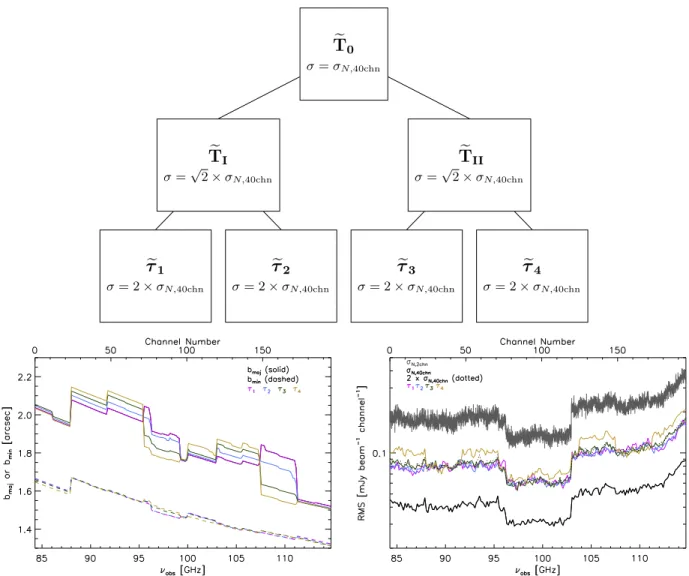
γN=0.25. The process is visualized as a tree diagram in the

top panel of Figure3.

In practice, we forgo the step of dividing T0 into subsets TI and TIIand begin by dividing T0into quarters t1through t4. The CASA measurement set represented by T0 contains visibility data corresponding to 11 frequency ranges, or spectral windows,23that have been stitched together from all available data so that the spectral windows in T0are ordered from lowest

to highest observed frequency, with no overlapping regions. (Please refer to Section 2.4 of Walter et al. 2016 for more details on the construction of T0.) For each spectral window in

T0, there are multiple blocks of visibility data corresponding to

the various execution blocks scheduled by ALMA for observing. Each block, in turn, is typically comprised of eight to nine scans that repeat 17 times to cover the entire spatial area of the mosaic. Using the CASA task split, we select and

Figure 3.Top: tree diagram illustrating the derivation of visibility data subsets TI, TII,t1,t2, t3, andt4from the original visibility data set T0, used to determine the noise-bias-free power spectrum,PT TI II, ( )k, and corresponding errordPT TI II, ( )k. The expected mean rms of the resulting image generated from each visibility data set is also labeled. Bottom left: beam major(solid curves) and minor (dashed curves) axes as a function of observed frequency for image subsets τ1,τ2,τ3, andτ4. Numbers

in the upper x-axis refer to the channel number of the data cube, which has been imaged with a factor of 40 rebinning in frequency. Bottom right: rms as a function of observed frequency. The upper x-axis is the same as in the bottom left panel.

23_{We do not refer to the four 1.875GHz spectral windows of the ALMA} sidebands.

distribute these scans evenly among four subsets. We repeat these steps for every block of scans and every spectral window and merge visibilities in the four subsets using the CASA task concat—followed by statwt, for a homogenous weighting system in the concatenated data—to produce the subsets t1, t2, t3, and t4. Our choice of dividing T0this way guards against

possible frequency and/or temporal biases, as each subset contains the full range of frequency (84–115 GHz)—required, moreover, so that all image cubes probe the same line-of-sight distance—and time (2016 December 2–21) covered by the observations. The splittings have also resulted in small (i.e., less than the 0 36 cell size in the gridded image cubes) variations in beam sizes between subsets(see bottom left panel in Figure 3), which is necessary when taking the cross-power

spectrum or performing other mathematical operations, like subtraction, between any two images.24

4. Results

4.1. Limits from Detected Sources 4.1.1. Mean Surface Brightness at 99GHz

A direct measurement of the mean CO surface brightness, áTCOñ, across observed frequencies νobs=84.3–114.8GHz

provides an empirical point of comparison to model predictions in the context of CO intensity mapping experiments at moderate redshifts, and also places a constraint on foreground emission for cosmic microwave background (CMB) experi-ments aiming to map spectral distortions at high redshift. We repeat the analysis performed for the ASPECS-Pilot program by Carilli et al. (2016) to place a lower limit on áTCOñ at νobs=99 GHz, based on blindly detected sources in the

ASPECS LP 3 mm survey.

Following Carilli et al. (2016), we consider the aggregate

emission from all observed CO transitions that contribute to the mean sky brightness at 99GHz. We begin by summing the line fluxes of the 16 blindly detected CO emission line candidates reported in GL19 to obtain a total CO flux of 6.91±0.19 Jy km s−1 or, equivalently, (2.280.06)´106 JyHz. Dividing this total flux by ΔνBWyields a total mean CO

flux densityá ñ =Sn (7.530.21)´10-5_{Jy. Finally, to derive} a mean surface brightness in units of μK, we apply the Rayleigh–Jeans approximation,áTCOñ ~1360á ñSn lobs2 ASblind=



0.55 0.02 μK, where λobs is the observed wavelength (in

units of cm) and A_Sblind is the survey area(in units of arcsec2) utilized in the line search, corresponding to the region of the mosaic where primary beam attenuation is less than 20%: 1.69×104arcsec2 at 99GHz. Following the prescription in Moster et al.(2011), we estimate a 19.5% relative uncertainty

on áTCOñdue to cosmic variance in the pencil beam survey by combining the fractional uncertainties25 calculated for each identified line entering into the above flux sum, given the survey depth in stellar mass, mean redshift, and survey volume probed by the respective J transition. Because Moster et al. (2011) estimated cosmic variance as the product of galaxy bias

and the dark matter cosmic variance, their prescription is strictly applicable here in the case where the galaxy bias is identical to the bias bCOof CO emission with respect to the

matter densityfield.

For ASPECS-Pilot, which consisted of a single∼1arcmin2 pointing with the same spectral coverage as ASPECS LP, áTCOñ was found to be 0.94±0.09μK at 99GHz (Carilli et al.

2016), which is a factor of 1.72 times greater than reported here

for ASPECS LP. Since the time of publication of that analysis, however, four of the 10 line candidates reported by ASPECS-Pilot(namely, 3 mm.4, 3 mm.7, 3 mm.8, and 3 mm.9 in Table 2 of Walter et al. 2016) have been reclassified as

“uncon-firmed”—i.e., likely spurious, given their narrow line widths— sources based on the improved line search algorithms developed inGL19and are excluded from the present analysis. Additionally, two of the ASPECS-Pilot line candidates (3 mm.6 and 3 mm.10) are outside the ASPECS LP survey coverage and similarly excluded. Thus, when including emission from only the four remaining confirmed sources from the original 10 sources listed in Walter et al. (2016), one

finds that the total observed CO flux scales linearly with the decrease in observed survey area, resulting in a revised áTCOñ =0.550.05 μK for ASPECS-Pilot, consistent with

our new measurement.

It is important to note that the measurement of áTCOñ presented here is considered a lower limit because the blind detections represent only a fraction of the total CO emission in the ASPECS LP survey volume; the fraction recovered by blind detections is determined by the sensitivity limit of the survey and the shape of the relevant CO LFs. We compute the mean CO surface brightness based on the observed CO(2–1), CO(3–2), and CO(4–3) LFs for ASPECS LP presented inD19

as follows: ( ) ( ) ( ( )) ( ( )) ( ( )) ( ( ))

ò

where DL, y, and DA,co refer, respectively, to the luminosity

distance, the derivative of the comoving radial distance with respect to the observed frequency (i.e., y=dc nd =

( ) ( )

lrest 1+ z 2 H z ), and the comoving angular diameter distance and are all evaluated at zcen,CO(J- -(J 1)). Here

( ( ( )))

F LCOJ- -J 1 is originally expressed as a function of the integrated source brightness temperature,L_CO¢ _{(J- -(J 1))} (in units of K km s−1pc2), F(LCO(J- -(J 1))¢), and is given in the logarithmic Schechter form

⎛ ⎝ ⎜⎜ ⎞_⎠⎟⎟ ( ) ( ) ( ) ( ( )) ( ( )) ( ( )) ( ( )) ( ( )) a F ¢ = F + ¢ ´ ¢ ¢ + - - -L L L L L

log log log

1 ln 10 log ln 10 . 18 J J J J J J J J J J 10 CO 1 10 10 CO 1 CO 1 CO 1 CO 1 10 * * *

We convert fromL_CO¢ _{(J- -(J 1))} toLCO(J- -(J 1))(in units of solar luminosity) via

( ) ( - -( ))= ´ - n (- -( )) ¢ (- -( ))

LCOJ J 1 3 10 11 3rest,COJ J 1 LCOJ J 1 19

from Carilli & Walter (2013). Fits to the LF data have

yielded Schechter parameters α, Φ_*, and LCO¢ (J- -(J 1))_{*, with}

24

Splitting T0must be done in a way that preserves the real and Fourier spaces probed by T0. For example, if T0 were split into two sets TI and TII that contained visibilities from the first and second half of the channels, respectively, in T0, then TI+TII=T0would still hold, but the images TIand

TIIwould each probe only half of the volume in T0.

25

The relative uncertainty on the mean CO(2–1), CO(3–2), and CO(4–3) surface brightnesses due to cosmic variance is 17%, 23%, and 54% for minimum stellar masses probed of 6×109_{, 2×10}10_{, and 3×10}10 _M

e,

uncertainties summarized in Table 3. Note that the faint-end slope,α, has been fixed at α=−0.2 for all LFs.

Integrating the LFs(Equation (17)) from an upper luminosity

limit Lupp¢ =1012 K km s−1pc

2 _{down to the mean 7σ line}

sensitivity26 L_min,7¢ _s in the respective redshift interval covered by each CO transition, which reflects the ASPECS LP detection threshold,27 yields a mean total surface brightness áTCO LF,7ñ s =0.49–1.78μK, where the quoted range reflects the uncertainty in the LF parameters; please see Table 4for a breakdown of the inferred áTCOñby J transition. Extending the lower limit of integration down to L′min=108K km s−1pc2at

all redshifts implies a total mean surface brightness of áTCO LFñ =0.72–2.24μK. Therefore, we estimate that our blind detections represent áTCO LF,7ñ s áTCO LFñ =68.1%–79.5% of the total CO surface brightness at this observed frequency.

4.1.2. CO Shot-noise Power

As with the limit on mean CO surface brightness, the blindly detected sources in Table 2can also be used to place a lower limit on the expected CO shot-noise power.

The total CO shot-noise power from only the detected sources, [PCO,COshot (kCO 2 1( - ))]det, will contain contributions from galaxies emitting in the observed transitions J=2, 3, and 4,

[ ( )] [ ( )] [ ( )] [ ( )] ( ) ( ) ( ) ( ) ( ) ( ) ( ) ( ) ( ) ( ) ( ) = + + - - - -- - -- - -P k P k P k P k , 20 CO,CO shot CO 2 1 det CO 2 1 ,CO 2 1 shot CO 2 1 det CO 3 2 ,CO 3 2shot CO 2 1 det CO 4 3 ,CO 4 3

shot

CO 2 1 det

where[PCO 3 2 ,CO 3 2shot(- ) (-)(kCO 2 1(-))]detand[PCO 4 3 ,CO 4 3shot(-) ( -)(kCO 2 1( -))]det

have been converted to the CO(2–1) frame using Equation (11).

Each term on the right-hand side of Equation (20) can be

determined analytically by summing the N individual line fluxes per the expression

⎛ ⎝ ⎜ ⎞ ⎠ ⎟ ( ) ( ( ))

å

where VSrefers to the survey volume at zcen,CO(J- -(J 1)). Note that the above expression for shot-noise power has units of surface brightness squared times volume(μK2(Mpc h−1)3) and is equal to the same value at all k, appropriate for a Poisson sampling of galaxies.

Starting with the CO(2–1), CO(3–2), and CO(4–3) source fluxes from GL19, reported in Table 2, we find, for the entire ASPECS LP3 mm survey volume used in the blind search, lower limits on the expected shot-noise power of [PCO 2 1 ,CO 2 1shot_{(- ) ( -)}(kCO 2 1₍- ₎)]det=63.64,[PCO 3 2 ,CO 3 2shot(- ) ( - )(kCO 3 2(- ))]det

= 98.49, and[PCO 4 3 ,CO 4 3shot(-) (-)(kCO 4 3(-))]det=1.05μK

2_{(Mpc h}−1₎3

, respectively. For the cropped region (black dotted square in Figure 1) corresponding to the volume used in the power

spectrum analysis, we find that the CO(2–1), CO(3–2), and CO(4–3) line emitters each give rise to a respective shot-noise power of 73.99, 71.06, and 1.21μK2(Mpc h−1)3. The slightly higher shot-noise power predicted in the cropped region for CO(2–1) and CO(4–3) is due to the decrease in volume after the crop; the CO(3–2) shot-noise power decreases due to the fact that two of thefive detected sources are located outside of the boundary of the cropped region. After converting the CO(3–2) and CO(4–3) shot-noise power into the CO(2–1) frame, we sum each contribution to arrive at a total shot-noise power at zcen=1.315 arising from

the blind detections: [PCO,CO(k ( - ))] =118.45 shot

CO 2 1 det and

113.24μK2 (Mpc h−1)3 for the full survey and cropped region, respectively.

Finally, we estimate the expected shot-noise power based on theD19CO LFs, ⎡ ⎣ ⎢ ⎤ ⎦ ⎥ ( ) ( ) ( ( )) ( ( )) ( ( )) ( ( )) ( ( ))

ò

and find that the detected sources (i.e., integrating Equation (22) down to the relevant 7σ line sensitivity limit)

recover 95.2%–97.7% of PCO 2 1 ,CO 2 1( - ) ( - )(k ( - )) shot

CO 2 1 , 98.6%– 99.7% of PCO 3 2 ,CO 3 2shot( - ) ( - )(kCO 3 2( - )), and 84.9%–96.0% of

( )

( - ) ( - ) ( - )

P_{CO 4 3 ,CO 4 3}shot kCO 4 3 . In total, the recovered fraction is 96.0%–98.6% ofPCO,CO(k ( - ))

shot

CO 2 1 .

Table 3

CO LF Schechter Parameters fromD19

Line Redshift α log₁₀F_* log₁₀L_*¢ [log10 (Mpc−3_dex−1_)] [log10 (K km s−1_pc2 )] (1) (2) (3) (4) (5) CO(2–1) 1.43 −0.2 (fixed) -2.79-+0.090.09 10.09-+0.090.10 CO(3–2) 2.61 −0.2 (fixed) -3.83-+0.120.13 10.60-+0.150.20 CO(4–3) 3.80 −0.2 (fixed) -3.43-+0.220.19 9.98-+0.140.22 Note.(1) Line transition. (2) Mean redshift of LF redshift bin. (3) Faint-end slope parameter in Equation(18). (4) Normalization parameter in Equation (18). (5) Characteristic luminosity parameter in Equation(18).

Table 4

Mean CO Surface Brightness Inferred from Schechter-form LFs

Line ( ( )) áTCOJ- -J 1 ñ ( ¢ = ¢Lmin Lmin,7s) ( ( )) áTCOJ- -J 1 ñ ( ¢ =Lmin 108K km s−1pc2) (μK) (μK) (1) (2) (3) CO(2–1) 0.53-+0.210.32 0.72-+0.250.38 CO(3–2) 0.25-+0.120.31 0.29-+0.130.33 CO(4–3) 0.12-+0.080.25 0.20-+0.110.32 Notes. (1) Line transition. (2) Mean CO surface brightness calculated by integrating Equation (17) with lower and upper limits of integration

¢ = ¢ s

Lmin Lmin,7 and Lupp¢ =1012 K km s−1.(3) Same as column (2) but for ¢ =

Lmin 108K km s−1pc

2

.

26

For reference, the mean 7σ line sensitivity for ASPECS in CO(2–1), CO(3–2), and CO(4–3) is 2.68×109 K km s−1pc2 (9.85 × 105 Le), 3.70×109 K km s−1pc2 (4.58 × 106 Le), and 3.93×109 K km s−1pc2 (1.15 × 107_L e), respectively. 27

The S/N threshold S/N…6.8 applied to the catalog of all possible line candidates(including candidates down to low S/N) yields the 16 high-fidelity detections presented in Table2.

4.2. Measurement of CO Autopower Spectrum at 0.001 z  4.5

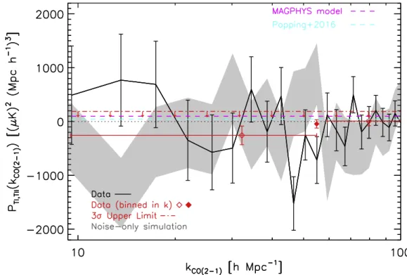
The noise-bias-free autopower spectrum, PCO,CO(kCO 2 1( -)), is presented in Figure4. We have averaged the power spectrum in linear bins of width dkCO 2 1( - )=2p r^,max=4.1h Mpc−1, measuring CO fluctuations on scales from kCO 2 1( -)~10 to 100h Mpc−1. Formally, the ASPECS survey volume provides access to 3D modes (i.e., modes containing both k_⊥ and k_P components) down to the fundamental mode kCO 2 1( -)= 4.1 h Mpc−1(see Table1), though the number of independent

modes Nm(=196, or one mode per every channel in the cube)

in this lowest wavenumber bin is small, and the resulting S/N on the power spectrum is low; it has been discarded in this analysis.

Errors on the power spectrum at each k_CO(2-1) bin, ( ( ))

d

á PCO,CO kCO 2 1- ñ, have been calculated using a 6° poly-nomialfit to the raw values calculated per Equation (16), as we

would expect ádPCO,CO(kCO 2 1( - ))ñ to approach a smooth function as the number of realizations of the noise-only cubes—( ( )t1 k -t2( ))k , ( ( )t3 k -t4( ))k , etc.—approaches infinity.

As an independent check on our error estimation, we also compute the noise-bias-free power spectrum of noise-only simulated data cubes, PN N, (kCO 2 1( - )), created with the CASA task simobserve. The output of simobserve is the CASA measurement sets, t1,N, t2,N, t3,N, and t4,N, that have been

generated to mock the ASPECS observational setup, including an identical mosaic pointing pattern and antenna configuration,

which determine the mosaic power pattern and synthesized beam sizes, respectively. We then produce dirty image data cubes with the same parameters(e.g., 40-channel rebinning in frequency) adopted for the real data and normalize the flux densities in each cube so that the rms of each frequency slice (or channel map) at a given νobs for a given simulated cube

(e.g., t1,N) is identical to the rms noise of the corresponding

data cube(e.g., τ1) at the same νobs(Figure3). In this way, we

have constructed noise-only simulated image cubes, t1,N–t4,N,

with noise properties similar to the real data cubesτ1–τ4. The

resulting noise-bias-free power spectrum of this simulated noise-only data set is shown alongside PCO,CO(kCO 2 1( - )) in Figure4.

To improve the S/N onPCO,CO(kCO 2 1( - )), we have averaged the power within individual wavenumber bins into two wider bins containing thefirst and second halves of the full kCO(2-1)

range and a third set containing all k_CO(2-1)bins in the available range. We then report the inverse-variance-weighted mean and corresponding inverse-variance-weighted error for the bin representing the power spectrum averaged across all Nb=23

bins from kCO(2-1)=9.55 to 100.05h Mpc−1,

( ( )) m ( )

áPCO,CO kCO 2 1- ñtot = -4577 K2 Mpc h-1 3. We compute similar quantities for the bin containing the lower half (9.55 h Mpc−1 kCO 2 1( - )54.98 h Mpc−1) of the modes only, áPCO,CO(kCO 2 1( - ))ñlow, and the upper half (59.20 h Mpc−1

( - )

kCO 2 1 100.05h Mpc−1) of the modes

Figure 4.Measurement of the noise-bias-free CO autopower spectrum(solid black curve),PCO,CO(kCO 2(-1)), in the ASPECS LP Band 3 survey. Error bars on ( (-))

PCO,COkCO 2 1 represent values from a polynomialfit to the raw errors,ádPCO,CO(kCO 2(-1))ñ, calculated from Equation(16). The inverse-variance-weighted mean CO power is plotted for two bins averaging modes in the upper and lower halves(open red diamonds) of probed kCO(2-1), as well as for a bin(filled red diamond)

containing the inverse-variance-weighted mean CO power for allkCO 2(-1)~10–100h Mpc−1. The 3σ upper limit, calculated using the uncertainty on the latter binned power spectrum, is plotted as the red dotted–dashed line. For comparison, the gray swath bounds the 1σ confidence region for the noise-bias-free power spectrum of a single realization of a noise-only simulated data cube from the CASA task simobserve, with the corresponding error bars calculated in the same way as for the real data. Theoretical predictions forPCO,COshot (kCO 2(-1))from Popping et al.(2016; cyan dashed line) and a model based on SED fitting of known sources in the ASPECS surveyfield (“MAGPHYS model”; magenta dashed line) are also plotted. A dotted black line that illustrates where the measured power is zero is drawn for reference.