ISSN 2282-6483
Cooperative Movement
and Prosperity
across Italian Regions
Michele Costa Flavio Delbono Francesco Linguiti
1
Cooperative Movement and Prosperity
across Italian Regions
Michele Costa
a)Flavio Delbono
a)Francesco Linguiti
b)a) Department of Economics, University of Bologna, P.za Scaravilli 2, 40126, Bologna, Italy ([email protected]; [email protected])
b) Area Studi, Legacoop, Via Guattani 9, 00161 Rome, Italy ([email protected])
Abstract
Our main objective is exploring the association between widespread prosperity and the presence of the cooperative movement at the regional level in Italy between 2010 and 2019. We summarize the widespread prosperity through an index originally proposed by Sen (1976) and we then perform a panel regression showing that there is a positive and significant association between such an index and the presence of the cooperative movement as captured by the relative size of cooperative employees. We also detect that the cooperative movement contributes to the regional prosperity more through its employment than in terms of the added value it generates. Moreover, the size of the cooperative presence significantly concurs to explain some large differentials among Italian regions.
JEL Codes: I31, J54
Keywords: social cohesion, regionalwell-being, income inequality, resilience
° We thank Giovanni Angelini, Elena Bontempi, Daniele Brusha, Guido Caselli, Giuseppe Cavaliere, Luca De Angelis, Luca Fanelli, Marco Mira d’Ercole, Sergio Pastorello, Stefano Zamagni, Vera Zamagni and participants in seminars held in (or run from) Bologna (Muec, Vancity, St. Mary University) for comments and suggestions. The usual disclaimer applies.
2
NON-TECHNICAL SUMMARY
Starting from the very fuzzy notion of “social cohesion”, we recognize that the “well-being” dimension is needed to establish a multidimensional index of social cohesion. Such a dimension, in turn, may be split into a set of indicators, among which we concentrate on income distribution as summarized by an Index of Widespread Prosperity (IWP, obtained by a combination of average household’s disposable income and a measure of their dispersion). Hence, we first analyze the regional patterns of this index and then we measure the impact of the regional cooperative magnitude on it. The benchmark is provided by all Italian regions in the period 2010-19.
In assessing well-being or the standard of living, a focus on income distribution is by now common practice. Even at the sub-national level, some measures of income inequality enter overall evaluations of economic inclusion (which in turn relates to well-being, social cohesion and standard of living) within communities. In the analysis of the Italian regions, the statistical evidence suggests that there is an increasingly negative correlation between average household disposable (real) income and the Gini value of its distribution. The IWP declines at the national level and in the vast majority of the regions.
In the econometric analysis uncovering the time frame 2010-19, we detect that, although cooperative employment and cooperative added-value are highly correlated, the latter is not significantly associated to regional prosperity. This is not surprising because a vast portion of cooperatives operates in labor-intensive sectors featured by relatively low added-value per worker. On the contrary, the size of the cooperative employment is highly and significantly associated to the IWP. Hence, we may cautiously claim that the Italian cooperative movement is entitled to be considered one of the relevant factors of regional prosperity, also potentially capable of reducing regional divides, at least in terms of employment and income disparities within territorial communities.
3
1. Introduction
The main objective of this paper is exploring the association between widespread prosperity1 and the size of the cooperative movement appropriately summarized. The
benchmark is provided by all Italian regions (Nuts 2) in the period 2010-19.
A measure of prosperity should capture an intuitive component of well-being, the one usually needed for a decent life in terms of freedom of choice in the access to resources. We are sympathizers of the capability approach (pioneered by Sen 1985 and 1986), where the individual well-being is defined as a function of the set of achievements (functionings), i.e., what one manages to do or to be in various life domains as well as the freedom one has in choosing among such achievements (capabilities). According to Sen (1985, p. 69), “the quality of life a person enjoys is not merely a matter of what he or she achieves, but also of what options the person has had the opportunity to choose from”. Hence, well-being is a multidimensional phenomenon consisting of several functionings, but what ultimately matters in Sen’s approach is the freedom of choosing among the many combinations of such subjective functionings. The well-known Human Development Index (HDI), firstly elaborated by the United Nations in 1990, is based on Sen’s theory. It considers three key capabilities to human development: a long and healthy life, knowledge and a decent standard of living2.
However, given the hard task to come up with selecting and measuring a group of capabilities, especially for sub-national layers of government, we follow here the so-called equivalent income approach, consisting in measuring well-being (also) in terms of an income metrics (Decancq et al. 2015). Of course, we are aware of several pitfalls of an income-based approach in trying to summarize attributes of a community which
1According to the Oxford Advanced Learner’s Dictionary, prosperity is “the state of being successful,
especially in making money”,
2 Brandolini (2008) provides an insightful discussion of multivariate indexes of living standard and
an application of the capability approach to four major European countries. For an interesting multidimensional approach to global well-being from a capability-based perspective in the last 150 years, see Prados de la Escosura (2021).
4
are doubtless multidimensional, but our ultimate goal is not about the perfection of an index of well-being, but the scrutiny of the relationship between a key component of well-being and our chosen main explanatory variable (the cooperative magnitude).
As for the choice of a measure of such component of well-being, let yit be the average
household disposable (real) income of the i-th population in year t and Git be the value
of the Gini index of the corresponding distribution. Let’s then define Yit = yit (1 – Git):
this can be interpreted as an Index of Widespread Prosperity (IWP), as it aims at catching an individually desirable attribute (high purchasing power as a proxy for prosperity), weighting positively the diffusion of close-to-the-average levels of such a power among households which belong to the relevant population. Yit has been
originally proposed in Sen (1976) in a seminal analysis of real national income: under some regularity conditions on social preferences, it may be (cardinally) interpreted as a social welfare function, in which Git measures the proportional loss in social welfare
to be imputed to inequality in the income distribution. Of course, any index hinging on Sen’s (1976) one can accommodate other indicators of, say, well-being, and variables other than real income, as well as measures of inequality of such variables different from the Gini one3.
To motivate the choice of a regional scale, one may notice that many countries exhibit notably large economic differences within their boundaries and such heterogeneity is obviously concealed in cross-country analyses4. Specifically, given the ultimate goal of our research, the distribution of cooperative firms around the world is drastically
3 See Decancq and Schokkaert (2016) for a step in that direction.
4 Various studies by (and within) OECD have shown that differences among regions belonging to the
same country may be larger than differences between countries. In 2013, for example, regional differences in the employment rate in Italy ranged from 40% in Campania to 73% in the autonomous province of Bolzano. This range is as large as the one observed across all OECD countries (Veneri and Murtin, 2016). Moreover, it is worthwhile noting that when looking at the inequality measures (e.g., Gini coefficients), regional inequality in income dimension may be relatively larger than in any other well-being dimension (as jobs, housing, education, health, access to services, civic engagement, environment, safety): Pinar (2019, p. 41, Table 3). In other words, income inequality matters not only
5
different across and within countries. Italy, which ranks top in international comparisons as for the economic impact of the cooperative presence, is no exception. Hence, a region-based breakdown of the Italian experience consistently follows.
The intuition driving the attempt of assessing the impact of the cooperative movement (also) on prosperity relies upon a sound background. Cooperative firms are featured by a democratic governance5, they do not discriminate across workers and/or members (as for gender or ethnicity, for example). Moreover, the empirical evidence suggests that they pursue a combination of revenue net of non-labour costs and employment, distribute a small portion of net revenues to members and tend to be more resilient than profit-making firms during downturns by stabilizing employment while sacrificing net revenues6. This countercyclical behaviour, by sustaining labour incomes - whose differences are notoriously the main source of overall personal income inequality at least in OECD countries - ends then with contrasting unemployment and the resulting wage edges between employees and unemployed people. In addition, the pay-ratio within cooperative firms, consortia and organizations is usually lower than within other organizational forms and this contributes to shrink income differentials among employees.
Furthermore, given the well-known structural small dimension of the vast majority of Italian enterprises, a comparative advantage is reaped by those territories capable of
networking their tiny production units. In carrying out such a task, the cooperative
movement excels and the outcome of such a coordination likely enhances the overall
5 See, for instance, Zamagni and Zamagni (2011) for a thoughtful account of the Italian cooperative
movement. To provide an order of magnitude of the economic presence of cooperative entities in the Italian economy, see Borzaga et al. (2019, p. 9-11). They elaborate figures retrieved from Istat datasets, according to which, in 2015, including subsidiaries, the cooperative companies account for about 1,215,000 employees (7.4% of total employment in the Italian private sector) and over 32 billion euros (4.4% of the corresponding added value).
6 See, for instance, Perotin (2012), Kruse (2016), Navarra (2016) and Caselli et al. (2021) for the
related empirical literature cited therein. In the cooperative companies, net revenues are mostly plough-back to increase indivisible reserves or increase capital and such a strategy clearly strengthens their financial sustainability. See Delbono and Reggiani (2013, p. 394) for some figures about the Italian experience before the financial crisis.
6
prosperity of the relevant territories (see Menzani and Zamagni, 2009 and Zamagni 2015).
These are the reasons why we did prefer the term movement instead of firms in the title of this paper: cooperative associations, indeed, continue to play a key role not only in representing cooperative companies (or groups7), but also in orienting them, promoting
mergers and workers-buy-out and other related supporting initiatives. Hence, one is reasonably induced to detect whether and how, in addition to feed other dimensions of social cohesion and well-being, the cooperative presence is linked to (our measure of) widespread prosperity. Of course, as argued above, given the remarkable differences in the cooperative magnitude across territories, our investigation makes sense especially at the regional level. As far as we know, this is the first attempt of measuring such a link, whatever the choice of the administrative layer.
The rest of the paper is organized as follows. In section 2 we briefly frame our contribution within the vast literature on social cohesion and well-being and then provide in section 3 a short description of how real income and its distribution jointly evolved across Italian regions. This is instrumental to the central question that we tackle in sections 4 and 5 where we present our analysis and comment the results. Section 6 concludes.
7 Cooperative groups are business groups which, according to Eurostat, are “associations of
enterprises bound together by legal and/or financial links. A group of enterprises can have more than one decision-making center, especially for policy on production, sales and profits. It may centralize certain aspects of financial management and taxation. It constitutes an economic entity which is empowered to make choices, particularly concerning the unit it comprises” (European Regulation 696/93). On this, see the detailed account of the Italian cooperatives in 2015 by Borzaga et al. (2019).
7
2. Social cohesion, well-being and prosperity
Despite being a hugely investigated word, the very notion of social cohesion still retains broad margins of ubiquity. One may agree with Chan et al. (2006) in envisaging two discourses about it: one coming from academic social sciences, while the other originated from policy-oriented research. Needless to say, the two discourses often overlap even if they ultimately point to different targets and audiences. At any rate, in both types of discourses, social cohesion is seen as a desirable attribute of a community and the term continues to enjoy an increasing popularity in debates well beyond the boundaries of scholarly qualified arguments, e.g., in political discussions8.
In this paper we pursue a much more limited goal than speculating on the most appropriate definition of social cohesion. We are interested in shedding light on an economic side of the intrinsically multifaceted concept of social cohesion, without questioning on it being a determinant, a consequence or a constituting element of the social cohesion itself9.
We concentrate on one component of the (in)equality dimension featuring most definitions of social cohesion, i.e., the one dealing with the distribution of material resources across members of a community, (real) income ranking top among such resources10. In assessing well-being or the standard of living, a focus on income
distribution is by now common practice. This is the case with 4 of the 12
8 This is attested also by the 40,000,000 results obtained by clicking social cohesion on Google (April,
27th, 2021, 12.50 am).
9 An updated survey is Schiefer and van der Noll (2017).
10 See Chan et al. (2006, p. 284) when citing proposals according to which income is a key index of
economic inclusion, which is in turn considered as one of the dimensions of social cohesion.
Economic inclusion belongs to the components of social cohesion that Durkheim (1893) labelled as “organic solidarity”, based on dissimilarity amongst individuals. Incidentally, the same test as the one reported in fn. 8, for economic inequality and income inequality delivers, respectively, 98,500,000 and 93,600,000 results. This upsurge of interest for inequality and its geography is widely reflected also in academic research, as carefully documented by Cavanaugh and Breau (2018).
8
recommendations forcefully put forward by Stiglitz et al. (2009) in their influential Report. Even at the sub-national level, some measures of income inequality enter overall evaluations of economic inclusion (which in turn relates to well-being, social cohesion and standard of living) within communities.
In this paper we specifically try to detect, at the regional level, the nature of the association between our index of widespread prosperity and a measure of the cooperative presence, taking account, as we shall see in section 4, other relevant characteristics of the Italian regions. In view of such an enquiry, we briefly investigate our index of widespread prosperity per se, across regions and over time, in section 3.
The related literature can be roughly split in two overlapping streams. The first one deals with various measures of well-being only across Italian areas; the second one addresses similar issues within sets of regions across countries.
As for the first group, the only paper related to ours is Cannari and D’Alessio (2002). They consider 16 Italian areas (mostly coinciding with regions) in the period 1995-2000. Relying on periodical Surveys of Household Income and Wealth run by the Bank of Italy, they estimate, inter alia, the Gini index of household’s disposable incomes which is then used to weight average incomes at the “regional” level (as in in the above Y). Ciani and Torrini (2019) use the same database as Cannari and D’Alessio (2002) to consider the time span between 2000 and 2016. They divide the country only in two macro areas and show that income inequality as measured by the Gini index is persistently greater in Southern Italy compared to the Centre-North area, although the gap seems to shrink in recent years (Ciani and Torrini, 2019, p. 11, Fig. 3a). Income distribution is also considered, for instance, by D’Urso et al. (2020), who focus on the measurement of well-being in Italian regions between 2010 and 2016, in Murias et al. (2012), who consider Italy and Spain mainly in 2005, and in Bertin et al. (2018) through selected opinions on 41 indicators of the Italian regions in 2012.
9
International samples of regions have been considered in other related empirical
contributions, usually by building and estimating various indices of well-being still accommodating measures of income inequality, in addition to indicators of other dimensions aimed at catching the living conditions of communities. We mention, for instance, Palomino (2019) and Pinar (2019). Both rely upon the OECD Regional Well-being Database (RWBD), available only for the years 2000 and 2014, which provides figures also about disposable income dispersion across households. The sample includes 395 OECD regions, and 213 European regions, respectively. Veneri and Murtin (2016) also compare a group of 209 OECD regions in the period 2003-12 by means of the MDLS (Multi-Dimensional Living Standards) index (see their box 3 for details about this OECD Database). They conclude that differences in households’ disposable income within regions are greater than differences in the other two components of the index (jobs and health), but the regional disparities in the MDLS exceed those in households’ disposable income.
Finally, it is worth mentioning Ezcurra (2009) and Bouvet (2010). The former investigates the relationship between income polarization and GDP growth in 61 EU regions between 1993 and 2003, reaching the conclusion that the association is negative. The latter considers a group of European regions between 1977 and 2003 to examine trends in income inequality. While interesting in many respects, both papers use GDP per capita to describe income distribution; this does not seem to us an advisable choice at the regional level. The discrepancy between the production’s location and the geographic distribution of factor revenue recipients is indeed usually greater, the smaller are the geographical units dividing a (not tiny) country. Hence, the use of GDP per capita instead of income casts some doubts on the interpretation of the resulting findings.
10
3. Regional widespread prosperity in Italy
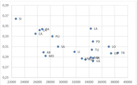
To proceed with a preliminary analysis of Yit, we plot 20 pairs in the income-Gini space
for all regions in 2010 (Fig. 1A, A mnemonics for Appendix) and 2019 (Fig. 2A). The data about regional income distributions are retrieved from official datasets (Eu-Silc, based too on households’ surveys). Since the Eu-Silc data cover up to 2017, we have estimated incomes and Gini values for 2018 and 2019. As for Gi, we employed the last
5 available values of Git (t = 2013-17) to obtain the two subsequent years via a linear
regression. As for as the regional average values of household disposable real incomes (yi), we obtain the 2018 values by means of the yearly rate of change between 2018
and 2017 (source: Istat, Regional accounts) and then we replicate the same update by using the values of 2018 to derive the 2019 ones. Moreover, since the datasets provide separate figures for the two autonomous provinces of Bolzano and Trento (which the region Trentino-Alto Adige is divided into), we average their data using population sizes (15+) as weights.
[Insert Figure 1A about here]
We used the Consumers Price Index (Istat, Foi(nt)) to deflate money incomes. It is noteworthy that using a national deflator yields an underestimate of households’ purchasing power in Southern regions where prices are notoriously lower than in the Centre-North of the country11.
[Insert Figure 2A about here]
While in 2010 the scatter plot does not exhibit any clear pattern, in 2019 a negative association between the regional real income and the corresponding Gini index
11
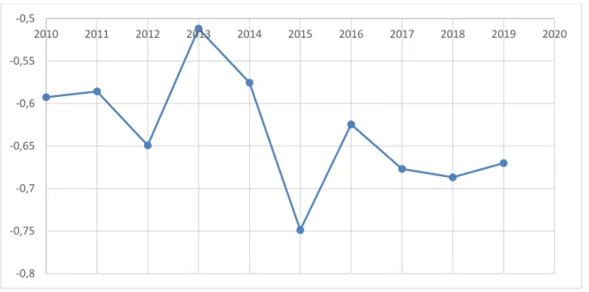
emerges quite clearly. Fig. 3 shows even more neatly that the correlation between regional real incomes and the Gini values of the corresponding distributions is negative and growing over time (the correlation coefficient increases from 0.59 to 0.67). A negative correlation has been detected also among countries12.
Figure 3. Correlation between Gini index and regional average incomes, 2010-19
Table 1 summarizes the (numerical) content of Figures 1 and 2 for the extreme years, appending the percentage changes in regional incomes, Gini values, as well as the value of Y, over the entire period.
12 In 2014, for instance, the correlation coefficient between average disposable income and
within-country income inequality (as measured by the Gini coefficient) is equal to − 0.79 in the European
countries (Pinar 2019, p. 43, fn. 25). -0,8 -0,75 -0,7 -0,65 -0,6 -0,55 -0,5 2010 2011 2012 2013 2014 2015 2016 2017 2018 2019 2020
12
Table 1. yit and Git; % changes in yit, Git and Yit; t = 2010, 2019; (*: special status regions)
2010 2019 2010/2019 yi Gi yi Gi % yi % Gi Yi Italy 32370 0,33 31483 0,343 -2,74 4,00 -4,66 Piedmont 34600 0,32 30966 0,314 -10,50 -1,88 -9,72 Valle d'Aosta* 34608 0,282 30716 0,313 -11,25 11,13 -15,13 Liguria 31746 0,3 31263 0,314 -1,52 4,60 -3,46 Lombardy 37067 0,31 36322 0,329 -2,01 6,13 -4,71 Trentino-Alto Adige* 38483 0,298 37097 0,310 -3,60 3,89 -5,19 Veneto 34637 0,288 35669 0,307 2,98 6,53 0,26 Friuli-Venezia Giulia* 33431 0,285 34310 0,284 2,63 -0,28 2,75 Emilia-Romagna 37427 0,297 35411 0,290 -5,39 -2,29 -4,47 Tuscany 34442 0,304 33957 0,332 -1,41 9,21 -5,37 Umbria 32888 0,287 33536 0,291 1,97 1,25 1,46 Marche 34278 0,289 33128 0,299 -3,36 3,39 -4,69 Lazio 34270 0,345 32331 0,378 -5,66 9,68 -10,47 Abruzzo 26936 0,299 27900 0,315 3,58 5,35 1,21 Molise 27249 0,292 27242 0,321 -0,03 9,86 -4,09 Campania 26327 0,342 24912 0,362 -5,38 5,73 -8,19 Apulia 28306 0,33 27622 0,334 -2,42 1,21 -3,00 Basilicata 26731 0,344 25837 0,358 -3,34 4,19 -5,46 Calabria 25686 0,335 25421 0,382 -1,03 14,15 -8,09 Sicily* 22643 0,364 22753 0,371 0,49 1,82 -0,56 Sardinia* 29196 0,31 28099 0,346 -3,76 11,48 -8,72
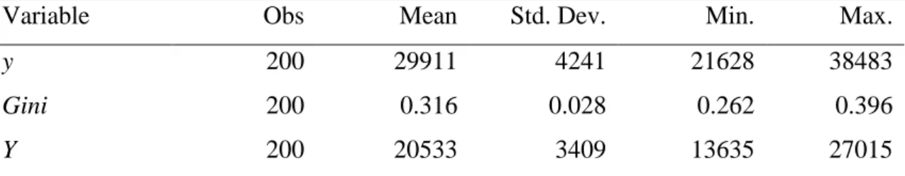
While the country as a whole has not recovered yet from pre-financial crisis levels (− 2.74% in real income) and the Gini index mildly moves up in the period, very different tendencies characterize the regional territories, both for the size of income contraction as well as for the variation in income dispersion. Table 2 collects the summary statistics of the tree variables under exam and to be used in the next section.
13
Table 2. Summary statistics
Variable Obs Mean Std. Dev. Min. Max.
y 200 29911 4241 21628 38483
Gini 200 0.316 0.028 0.262 0.396
Y 200 20533 3409 13635 27015
Unsurprisingly, the Coefficient of Variation of Y exceeds the one of y, supporting our choice of the former instead of the latter to capture differences in regional prosperity.
The Southern regions (including islands) continue to experience more uneven distributions around a lower real income than the Centre-North ones13. The country as
a whole performs quite poorly and, given the relative stability of the national Gini value, the driving factor seems to lay in the conspicuous fall in Italian GDP and real revenues observed after the financial crisis. Only a few regional territories experience (tiny) positive variations in Yi, the greatest of those being Umbria.
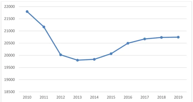
Fig. 4A visualizes the remarkable decrease in the average regional Y between 2010 and 2013, followed by a modest recoupment. Such a pattern is accompanied by an increase over time in the standard deviation of Y.
[Insert Figure 4A about here]
In Fig. 5A, we plot, for each region, the difference between its Yi and the unweighted
average value of all Yi, in the two extreme years of our time frame. The territorial gap
(Centre-North vs South) is confirmed once again. Moreover, it is worth underscoring
13 This is the conclusion reached also in Mussida and Parisi (2020) and Doran and Jordan (2013).
However, in Doran and Jordan (2013, p. 27) the real gross value added per capita, instead of real income per capita, is used to measure living standards for each region. Hence, the abovementioned comments about this choice applies also to their findings.
14
the generalized increase in the size of differentials wrt to the average (whatever their sign) in the period.
[Insert Figure 5A about here]
4. Methodology and empirical analysis
For the arguments provided in the introductory section, we conjecture the presence of a positive association between the chosen index of regional widespread prosperity (Y) and the size of the cooperative movement in terms of cooperative employees and/or added value obtained by cooperative organizations.
We obtain novel data on the regional cooperative presence by elaborating the balance sheets from the Bureau van Dijk-Aida dataset, whereas we retrieve all the other data from Istat (Labor Force Survey, in Italian). As for the interpretation of figures about the cooperative employment figures, it is worth stressing that we collect data about employees of cooperative firms and cooperative groups which are registered in the various regions. Of course, some of them, especially the largest ones, employ labour force also outside the regional boundaries. This means that we shall emphasize the economic consequences of decisions taken in the corporate headquarters located in the relevant region, being obviously aware that they yield economic effects also elsewhere. However, the territorial gap between the company’s location and the location of its employees is very small: in 2015, 99.6% of Italian cooperatives (and almost 85% of groups controlled by cooperatives) operate only in the region where they are registered (Borzaga et al. 2019, p. 10). Hence, we shall summarize the regional cooperative magnitude with the following variables14:
Cooperative employment (CEM): cooperative employees out of pop[15, 64].
15
Cooperative Added Value (CAV): cooperative added value out of regional GDP.
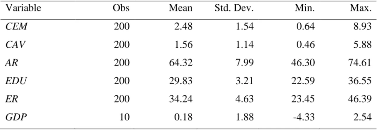
To complete the construction of the dataset to be used, in addition to the one collected in Table 2, the choice of the other relevant variables reflects a broadly consolidated empirical literature. Indeed, various indicators capturing demographic factors (as the elderly dependence rate, life expectancy, mortality rates), the share of population with at least secondary or third education, the participation in the labour market ((un)employment rate, activity rates) and real GDP have been variously included into multidimensional indexes of well-being15. Here we select the following variables:
Activity Rate (AR): active pop[15, 64] out of pop[15 ,64].
Education (EDU): pop[25, 64] with at least secondary education out of pop[15, 64]. Elderly Rate (ER): population 65+ out of pop[15, 64].
Italian Gross Domestic Product yearly rate of growth (GDP).
Table 3. Summary statistics
Variable Obs Mean Std. Dev. Min. Max.
CEM 200 2.48 1.54 0.64 8.93 CAV 200 1.56 1.14 0.46 5.88 AR 200 64.32 7.99 46.30 74.61 EDU 200 29.83 3.21 22.59 36.55 ER 200 34.24 4.63 23.45 46.39 GDP 10 0.18 1.88 -4.33 2.54
15 See, for instance, Murias et al. (2012), Bertin et al. (2018), Pinar (2018), Palomino (2019), Mussida
and Parisi (2020) and D’Urso et al. (2020). Notice, however, that the measures of households’ income distribution (averages and/or indices of dispersion) are included among the indicators of well-being, whereas in our analysis such measures are embedded into an index (Yit) that needs to be analysed wrt
16
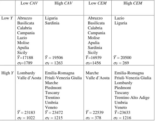
We begin by dividing the Italian regions into two groups according to their CAV (summarized by the mean over the period) wrt to the median. By means of the same criterion we classify regions wrt the median Y. The resulting Table 4 (where 𝑌̅ and Y
are the mean and the standard deviation of Y, respectively, in the relevant group between 2010 and 2019) shows that 8 low CAV regions out of 10 display also a low value of Y and 8 high CAV regions out of 10 feature also a high value of Y.
Very similar conclusions emerge with a taxonomy based on median CEM: 8 regions out of 10 share low values of CEM as well Y and 8 regions out of 10 share high values of both. Only four regions are located differently wrt to the classification based on median CAV.
Table 4. Italian regions wrt to Y and CAV and wrt to Y and CEM, 2010-2019
Low CAV High CAV Low CEM High CEM
Low Y Abruzzo Basilicata Calabria Campania Lazio Molise Apulia Sicily 𝑌̅=17188 Y=1789 Liguria Sardinia 𝑌̅ = 19506 Y = 1263 Abruzzo Basilicata Calabria Campania Molise Apulia Sardinia Sicily 𝑌̅=16939 Y=1456 Lazio Liguria 𝑌 ̅ = 20500 Y = 269 High Y Lombardy Valle d’Aosta 𝑌 ̅ = 23183 Y = 1022 Emilia-Romagna Friuli-Venezia Giulia Marche Piedmont Tuscany Trentino Umbria Veneto 𝑌 ̅ = 23472 Y = 1215 Marche Valle d’Aosta 𝑌 ̅ = 22539 Y = 378 Emilia-Romagna Friuli-Venezia Giulia Lombardy Piedmont Tuscany
Trentino Alto Adige Umbria
Veneto 𝑌̅=23633 Y = 1216
17
In either case, we can firmly reject the hypothesis of independence between regional widespread prosperity and either CAV or CEM. This descriptive result is confirmed by the statistics test 2=1 = 7.20, with associated probability p(2) = 0.0073, as well as
by Fisher’s exact test, with probability p = 0.011, which looks appropriate with fairly small samples as ours.
We now resort to a panel analysis allowing us to catch both the spatial and the temporal dimension of our data. Given the nature of our balanced panel, to test the aforementioned conjecture, we run the following linear panel regression:
Yi t = + Yi,t-1 + Xit’ + Zt’ + i + it (1)
where Xit is the vector of variables at time t described in Table 3, Zt is the vector of
time-dependent, region-invariant variables, i are regional fixed effects and it is the
residual component. The dependent variable Yit = yit (1 – Git) is central to our research
and has been illustrated in previous sections (and its summary statistics is in Table 2).
The presence of Yi,t-1 captures the alleged dynamics of Y, without ignoring regional
differentials. Some region-specific characteristics, such as the ones belonging to one of three geographic subsets (North, Centre and South) or being ordinary status type, or special status (the 5 starred regions in Table 1), are included in the regional fixed effects
i .
As for Zt, we consider the Italian real GDP yearly growth rate (GDP), whose statistics
is also summarized in Table 3. To ease the interpretation of the variables X and Z, all the above series are multiplied by hundred.
18
5. Results
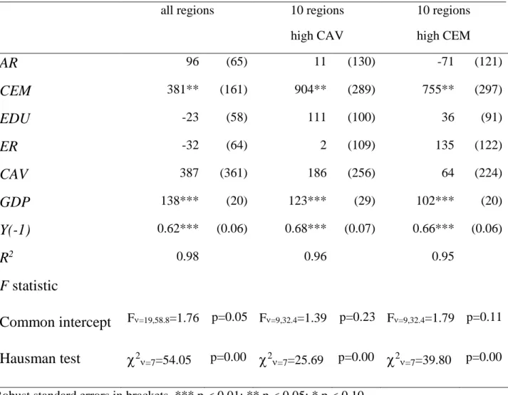
In Table 5 we report the OLS estimates of eq. (1), distinguishing the entire group of regions from the relative subsets of the 10 ones featured by a high CAV and by a high CEM. The Hausman test for random effects vs fixed effects, reported in the last row of Table 5, indicates a strong preference for the fixed effects model to be used below. Notice that including lagged values of Y among the regressors allows us to consider the presence of autocorrelation; however, it cannot but lead a strong heteroscedasticity requiring us to resort to robust standard errors that we calculate by means of the Arellano HAC estimator.
Table 5. Panel regression, Italian regions, 2010-19
Dependent variable: Y
all regions 10 regions
high CAV 10 regions high CEM AR 96 (65) 11 (130) -71 (121) CEM 381** (161) 904** (289) 755** (297) EDU -23 (58) 111 (100) 36 (91) ER -32 (64) 2 (109) 135 (122) CAV 387 (361) 186 (256) 64 (224) GDP 138*** (20) 123*** (29) 102*** (20) Y(-1) 0.62*** (0.06) 0.68*** (0.07) 0.66*** (0.06) R2 0.98 0.96 0.95 F statistic Common intercept F=19,58.8=1.76 p=0.05 F=9,32.4=1.39 p=0.23 F=9,32.4=1.79 p=0.11 Hausman test 2=7=54.05 p=0.00 2=7=25.69 p=0.00 2=7=39.80 p=0.00 Robust standard errors in brackets. *** p < 0.01; ** p < 0.05; * p < 0.10
19
As we expect, Y(-1), which greatly varies across territories, captures a portion of the differentials measured by the regional fixed effects i . In the analysis of our 20 regions,
the joint Welch’s F test (reported in the last but one row of Table 5) rejects the presence of a unique intercept, hinting at significant regional fixed effects i. Looking at the two
subsets of regions featured by similar levels of CAV or CEM, the Welch’s F test does not suggest any longer to reject the hypothesis of a common intercept and this looks consistent with dealing now with less heterogeneous groups of regions.
The significant differences across Italian regions, often documented by other researches, emerge also in our analysis. This is also true regarding the relevance of their geographic position and the ordinary vs special type of their statutes, as jointly specified by Y(-1) and i.
GDP and Y(-1) are the most relevant explanatory variables, which positively and
significantly affect Y. A unitary increase in GDP yields an average increase of 100
euros in Y, which instead rises by 62 euros if Y goes up by 100 euros the year before.
In addition to GDP and Y(-1), the most important variable is CEM: an increasing cooperative employment is positively and significantly associated to increases in Y: a unitary increase in CEM raises Y by about 380 euros.
As for the other variables, no significant association is therefore detected: conditionally on the effects of GDP, Y(-1) and CEM, neither the education ratio, nor the elderly rate seems to affect the regional prosperity. The same irrelevance is detected in the relationship between prosperity and the added value obtained within the cooperative boundaries. Indeed, it is worth noting that while CEM and CAV are highly correlated, the latter, as opposed to the former, is not significant. This is not surprising because it is well known that a vast portion of cooperatives operate in labor-intensive sectors featured by a relatively low added-value per worker16.
16 According to Istat datasets, in 2015, for instance, the average added value per worker was 45,605 euros in the overall Italian companies, whereas in the cooperative subset of them (including cooperative groups), it was
20
If we estimate the equation (1) by restricting the sample to the 10 regions with high
CAV (see Table 4), we obtain the results reported in columns 4-5 of Table 5. The
previous findings stemming from the panel regression within the complete sample are strengthened. We notice that the impact of cooperative employment on prosperity more than doubles compared to the nation-wide one: for the top 10 regions in terms of CAV, a unitary increase in CEM increases Y by more than 900 euros. This finding is consistent with the tests performed relatively to Table 4 and indicates that the regions with the highest cooperative presence exhibit the highest levels of prosperity.
The same conclusions are reached if, instead of top-ranked regions in terms of CAV, we would focus on those featured by high levels of CEM. The cooperative presence is confirmed to be again positively and significantly associated to the regional prosperity.
6. Concluding remarks
Let us summarize the track followed in this paper. We briefly outlined the role of well-being in the broad research area explored within the fuzzy boundaries of “social cohesion” by both academic and policy-oriented scholars. We acknowledge and recognize in the literature that the “well-being” dimension is needed to establish a multidimensional index of social cohesion. Such a dimension, in turn, may be split into a set of indicators. The indicator that we choose to concentrate on is income distribution as summarized by our index of widespread prosperity. Hence, we first analyze the regional patterns of this index. Then, we measure the impact of the regional cooperative presence on it.
While testing the impact on prosperity of the cooperative movement as proxied by the relative number of its employees, we conjecture that the cooperative presence may also yield effects on other dimensions of well-being and social cohesion. Therefore, a richer
24,851 euros (Borzaga et. al. 2019, p. 11). These figures about cooperative employees and added value exclude financial and insurance activities; for instance, they ignore the cooperative credit banks.
21
set of indicators of the cooperative presence may likely strengthen our findings as well as positively affect other dimensions considered in composite indexes. This is left for future research.
In the first part of this paper we show that Italian regions display wide differences in many social and economic spaces, including the distribution of prosperity across households. This amounts to confirming the conclusion reached by a vast literature using many indices of well-being and social cohesion. Within an income-based approach to well-being, we initially detected that income inequality rises in almost all Italian regions, especially in the South, and the presence of a negative (and increasing over time) correlation between income levels and the Gini values17. Lastly, the regional widespread prosperity declines almost everywhere, especially in the South.
We then focus specifically on the contribution of a phenomenon like the Italian cooperative movement on a key dimension of regional well-being as the one captured by Y. Within such a relatively narrow frame and in a limited time span, notwithstanding the simplicity of our model, our new findings look encouraging and arguably worth further investigation. Indeed, we detect a large and significant association between the size of the cooperative employment and our index of widespread prosperity and such an association is not mitigated by standard economic and socio-demographic control variables entering our panel regression. Hence, we may cautiously claim that the Italian cooperative movement looks entitled to be considered one of the relevant factors of regional prosperity, also potentially capable of reducing regional divides, at least in terms of employment and income disparities within communities. Moreover, our findings suggest also an apparent positive association between the size of the regional cooperative movement and the resilience of regional economic system18 with respect to sever shocks like the ongoing pandemics-driven one.
17 This evidence echoes some findings of the vast research stream on the macroeconomic relationship
between growth and income inequality: see, for instance, Naguib (2017) for an interesting empirical research and an updated survey.
23
Appendix
Figure 1A. Gini index and average income, Italian regions, 2010
Figure 2A. Gini index and average income, Italian regions, 2019
PD VA LI LO TR VE FVG ER TU UM MA LA AB MO CA PU BA CA SI SA 0,25 0,27 0,29 0,31 0,33 0,35 0,37 0,39 22000 24000 26000 28000 30000 32000 34000 36000 38000 40000 PD VALI LO TR VE FVG ER TU UM MA LA AB MO CA PU BA CA SI SA 0,25 0,27 0,29 0,31 0,33 0,35 0,37 0,39 22000 24000 26000 28000 30000 32000 34000 36000 38000 40000
24
Figure 4A. Average Y, 2010-19
Figure 5A. Differences between Yi and average Y, 2010 and 2019
18500 19000 19500 20000 20500 21000 21500 22000 2010 2011 2012 2013 2014 2015 2016 2017 2018 2019 -8000 -6000 -4000 -2000 0 2000 4000 6000 2010 2019
25
References
Alaimo, L., A. Arcagni, M. Fattore, F. Maggino and V. Quondamstefano (2020), “Measuring Equitable and Sustainable Well-Being in Italian Regions: The Non-aggregative Approach”, Social Indicators Research, doi.org/10.1007/s11205-020-02388-7.
Bertin, G., L. Carrino and S. Giove (2018), “The Italian Regional Well-Being in a Multi-expert Non-additive Perspective”, Social Indicators Research, 135, 15-51.
Borzaga, C., M. Calzaroni, C. Carini and M. Lori (2019), “Italian cooperatives: an analysis of their economic performances, employment characteristics and innovation processes based on combined used of official data”, CIRIEC WP 2019/06.
Bouvet, F. (2010), “EMU and the dynamics of regional per capita income inequality in
Europe”, Journal of Economic Inequality, 8, 323-44.
Brandolini, A. (2008). "On applying synthetic indices of multidimensional well-being: health and income inequalities in selected EU countries", Bank of Italy, WP 668.
Cannari, L. and G. D’Alessio (2002), “La distribuzione del reddito e della ricchezza nelle regioni italiane”, Rivista economica del Mezzogiorno, 16, 809-47.
Caselli, G., M. Costa and F. Delbono (2021), “What Do Cooperative Firms Maximize, if at All? Evidence from Emilia-Romagna in the pre-Covid Decade”, Department of Economics WP 1159, University of Bologna.
Cavanaugh, A. and S. Breau (2018), “Locating geographies of inequality: publication trends across OECD countries”, Regional Studies, 52, 1225-36.
Chan, J. H.-P. To and E. Chan (2006), “Reconsidering Social Cohesion: Developing a Definition and Analytical Framework for Empirical Research”, Social Indicators
Research, 75, 273-302.
Ciani, E. and R. Torrini (2019), “The geography of Italian income inequality: recent trends and the role of employment”, Bank of Italy Occasional Paper 492.
26
Costa, M. and F. Delbono (2021), “Cooperative Movement and Economic Resilience across Italian Regions: 2008-20”, mimeo.
Decancq, K., M. Fleurbaey and E. Schokkaert (2015), “Inequality, Income, and Well-Being”, in Atkinson, A. and F. Bourguignon (eds.), Handbook of Income Distribution, Volume 2A, Amsterdam, Elsevier, pp. 73-140.
Decancq, K. and E. Schokkaert (2016), “Beyond GDP: Using Equivalent Incomes to Measure Well-Being in Europe”, Social Indicators Research, 126, 1-55.
Delbono, F. and C. Reggiani (2013), “Cooperative firms and the crisis: evidence from some Italian mixed oligopolies”, Annals of Public and Cooperative Economics, 84, 383-97.
Doran J. and D. Jordan (2013), “Decomposing European NUTS2 regional inequality from 1980 to 2009”, Journal of Economic Studies, 40, 22-38.
Durkheim, E. (1893), De la division du travail social, Paris, Felix Alcan.
D’Urso, P., L. Alaimo, L. De Giovanni and R. Massari (2020), “Well-Being in the Italian Regions Over Time”, Social Indicators Research,
doi.org/10.1007/s11205-020-02384-x.
Ezcurra, R. (2009), “Does Income Polarization Affect Economic Growth? The Case of the European Regions”, Regional Studies, 43, 267-85.
Kruse, D. (2016), “Does employee ownership improve performance?”, IZA World of Labor 311.
Menzani, T. and V. Zamagni (2009), “Cooperative Networks in the Italian Economy”,
Enterprise and Society, 11, 98-127.
Murias, P., S. Novello and F. Martinez (2012), “The Regions of Economic Well-being in Italy and Spain”, Regional Studies, 46, 793-816.
Mussida, C. and M. L. Parisi (2020), “Features of Personal Income Inequality Before and During the Crisis: An Analysis of Italian Regions”, Regional Studies, 54, 472-82.
Naguib, C. (2017), “The Relationship between Inequality and Growth: Evidence from New Data”, Swiss Journal of Economics and Statistics, 153, 183-225.
27
Navarra, C. (2016), “Employment stabilization inside firms: an empirical investigation of worker cooperatives”, Annals of Public and Cooperative Economics, 87, 563-85. Palomino, J. (2019), “Regional well-being in the OECD disparities and convergence profiles”, Journal of Economic Inequality, 17, 195-218.
Perotin, V. (2012), “The performance of workers cooperatives”, in Battilani P. and H. Schroter (Eds.), The cooperative business movement, 1950 to the present, Cambridge, Cambridge University Press.
Pinar, M. (2019), “Multidimensional Well‑Being and Inequality Across the European Regions with Alternative Interactions Between the Well‑Being Dimensions”, Social
Indicators Research, 144, 31-72.
Prados de la Escosura, L. (2021), “Inequality Beyond GDP: A Long View”, CEPR DP 15853.
Schiefer, D. and J. van der Noll (2017), “The Essentials of Social Cohesion: A Literature Review”, Social Indicators Research, 132, 579-603.
Sen, A. (1976), “Real National Income”, Review of Economic Studies, 43, 19-39.
Sen, A. (1985), Commodities and Capabilities, Amsterdam, North-Holland.
Sen, A. (1986), The Standard of Living, Cambridge, Cambridge University Press.
Stiglitz, J.E., A. Sen and J.-P. Fitoussi (2009), Technical Report by the Commission on
the Measurement of Economic Performance and Social Progress.
Veneri, P. and F. Murtin (2016), “Where is Inclusive Growth Happening? Mapping Multi-dimensional Living Standards in OECD Regions”, OECD WP 2016/1.
Zamagni, S. and V. Zamagni (2011), Cooperative Enterprise, Chelthenaum, Edward Elgar.
Zamagni, V. (2015), “The Cooperative Movement”, in Jones, E. and G. Pasquino (Eds.), The Oxford Handbook of Italian Politics, Oxford, Oxford University Press.
28
Zamagni, V. (2018), L'economia italiana nell' eta' della globalizzazione, Bologna, Il Mulino.