Contents lists available atScienceDirect
Advances in Engineering Software
journal homepage:www.elsevier.com/locate/advengsoftAn interval finite element method for the analysis of structures with
spatially varying uncertainties
Alba Sofi
a,b,⁎, Eugenia Romeo
c, Olga Barrera
d,e, Alan Cocks
eaDepartment of Architecture and Territory and Inter-University Centre of Theoretical and Experimental Dynamics, University "Mediterranea" of Reggio Calabria, Salita Melissari, Feo di Vito, 89124 Reggio Calabria, Italy
bVisiting Fellow at the Department of Engineering Science, University of Oxford, Parks Road, OX13PJ, Oxford UK
cDepartment of Civil, Energy, Environmental and Materials Engineering, University “Mediterranea” of Reggio Calabria, Via Graziella, Località Feo di Vito, 89124 Reggio Calabria, Italy
dSchool of Engineering, Computing and Mathematics, Oxford Brookes University, Wheatley Campus, Wheatley, Oxon (UK) OX33 1HX eDepartment of Engineering Science, University of Oxford, Parks Road, OX13PJ, Oxford UK
A R T I C L E I N F O Keywords:
Finite element method Interval field
Response surface approach Lower bound and upper bound ABAQUS
A B S T R A C T
Finite element analysis of linear-elastic structures with spatially varying uncertain properties is addressed within the framework of the interval model of uncertainty. Resorting to a recently proposed interval field model, the uncertain properties are expressed as the superposition of deterministic basis functions weighted by particular unitary intervals. An Interval Finite Element Method (IFEM) incorporating the interval field representation of uncertainties is formulated by applying an interval extension in conjunction with the standard energy approach. Uncertainty propagation analysis is performed by adopting a response surface approach which provides ap-proximate explicit expressions of response bounds requiring only a few deterministic analyses. Then, the whole procedure is implemented in ABAQUS’ environment by coding User Subroutines and Python scripts.
2D plane stress and bending problems involving uncertain Young's modulus of the material are analyzed. The accuracy of the proposed IFEM as well as response variability under spatially dependent uncertainty are in-vestigated.
1. Introduction
Uncertainty assessment of structural systems is attracting growing interest in various engineering and industrial fields. Indeed, it is widely recognized that uncertainties affecting model parameters, such as ma-terial or geometrical properties, may have a significant influence on the performance of engineering systems [1,2]. One of the most urgent challenges in the context of non-deterministic analysis is to develop efficient and robust algorithms for predicting the influence of uncertain parameters on the response of real world large-scale systems. Over the last decades, much research effort has been devoted to incorporating uncertainties into the standard finite element method (FEM) in order to exploit all capabilities of deterministic FE solvers as well as the in-creasing power of available computational resources.
The extension of the classical FEM to problems involving un-certainties modeled as random variables or random fields led to the well-known Stochastic Finite Element Method (SFEM), which may be viewed nowadays as the most powerful tool in the field of computa-tional stochastic mechanics (see e.g.,[3,4]). Many variants of the SFEM
have been proposed in the literature, while much less attention has been devoted to the development of specialized software for the ana-lysis of large-scale stochastic problems. To address the need for prob-abilistic FE analysis in practical engineering, ANSYS Inc. released two tools, namely the ANSYS Probabilistic Design System and the ANSYS DesignXplorer[5]. Such tools enable random input variables to be ac-counted for, such as material properties, boundary conditions, loads and geometry, and to handle several types of analysis. However, the description of uncertainties is limited to the use of random variables. A random field[6]representation is required to take into account the inherent spatial dependency of non-deterministic properties which may significantly affect the reliability of a design. A stochastic FE library (StoFEL) has also been coupled with ANSYS for predicting response variability[7]. Among specialized software for SFE analysis, it is worth mentioning computational stochastic structural analysis (COSSAN)[8], numerical evaluation of stochastic structures under stress (NESSUS) [9], and finite element reliability using MATLAB (FERUM)[10]. To the extent of the authors' knowledge, only Shang et al. [11]faced the challenging task of incorporating uncertain mechanical properties
https://doi.org/10.1016/j.advengsoft.2018.11.001
Received 25 May 2018; Received in revised form 18 September 2018; Accepted 5 November 2018
⁎Corresponding author.
E-mail addresses:[email protected](A. Sofi),[email protected](E. Romeo),[email protected](O. Barrera),[email protected](A. Cocks).
Advances in Engineering Software 128 (2019) 1–19
Available online 22 November 2018
0965-9978/ © 2018 Elsevier Ltd. All rights reserved.
Nomenclature
Ai n − component vector whose j − th element is 1/Ai,j
Ai,j unknown coefficients of the proposed response surface
a0i,j midpoint of the i − th interval deviationUi jI,
B(h)(x) strain-displacement matrix
BI(x) dimensionless interval fluctuation around the midpoint E
0
of EI(x)
Bi,j unknown coefficients of the proposed response surface b(x) body forces
CB parameter governing the degree of uncertainty of the
in-terval field
c.i.u.[•] coefficient of interval uncertainty of •
DI(x) interval constitutive matrix D0 nominal constitutive matrix
Di(x) deviation matrix associated with the i-th extra unitary
in-terval
d(h)I interval nodal displacement vector of the h-th element
E0 midpoint of EI(x)
EI(x) interval Young's modulus field
E(LB)(x,y) sample of Young's modulus which yields the lower bound
of the response quantity of interest
E(UB)(x,y) sample of Young's modulus which yields the upper bound
of the response quantity of interest
e^I interval vector collecting M extra unitary intervals e^iI i − th extra unitary interval
e^h k, (LB)
vector of the combinations of the endpoints of the extra
unitary intervals e^h k i(LB), , which give the lower bound of the
k − th component of the interval stress within the h − th
finite element
e^h k(UB), vector of the combinations of the endpoints of the extra
unitary intervals e^h k i(UB), , which give the upper bound of the
k − th component of the interval stress within the h − th
finite element
F global nodal force vector
FVI interval field variable
f(h) nodal force vector of the h − th finite element KI interval global stiffness matrix
K0 nominal global stiffness matrix Ki i − th global deviation stiffness matrix
k(h)I interval stiffness matrix of the h − th finite element kh
0
( ) nominal stiffness matrix of the h − th finite element
ki( )h i − th deviation matrix of the h − th finite element
I (superscript) denotes interval variables
L(h) connectivity matrix
L plate width
LeI interval external work
lBx(lB) parameter ruling the spatial dependency of the uncertain property along the x- direction
lBy(lB) parameter ruling the spatial dependency of the uncertain property along the y-direction
M truncation order of the Karhunen–Loève-like expansion mid{•} midpoint of •
max {•} maximum of • min {•} minimum of •
N number of finite elements
N(h)(x) shape function matrix
NG number of integration points
n number of degrees-of-freedom
O(x, y, z) Cartesian coordinate system
real numbers
S boundary surface of the continuous body
St free surface of the continuous body
Su constrained surface of the continuous body
s ( )h i,( )x vector collecting the sensitivities s i,( )x
k( )h of the interval stress components k( )h I( )x within the h − th finite element
with respect to the i − th extra unitary interval
t(x) surface forces
UI interval global displacement vector U0 nominal displacement vector
U(i) + displacement vector obtained setting all the extra unitary
intervals equal to zero except the i − th which is set to 1
U(i) − displacement vector obtained setting all the extra unitary
intervals equal to zero except the i − th which is set to − 1
UjI j − th interval displacement component
U0,j j − th nominal displacement component Ui jI
, i − th interval deviation of the j − th displacement com-ponent
uu(x) displacements imposed on the constrained surface u(h)I(x) displacement field within the h − th finite element
V volume of the continuous body
Vh volume of the h − th finite element
XG,j vector listing the coordinates of the j − th integration point
x position vector
ΓB(x,ξ) spatial dependency function ΔE(x) deviation amplitude of EI(x) ΔB(x) deviation amplitude of BI(x)
Δai,j deviation amplitude of the i − th interval deviationUi jI,
ε(h)I(x) interval strain field within the h − th finite element
εR(%) absolute percentage error affecting the estimate of R
λi i − th eigenvalue of ΓB(x,ξ) ξ position vector
ξ, η Cartesian coordinates
ΠI Interval Total Potential Energy functional Σ solution set
σ(h)I(x) interval stress field within the h − th finite element
ΦI interval elastic strain energy
ψi(x) i − th eigenfunction of ΓB(x,ξ) |•| absolute value of •
Overbar denotes the upper bound of an interval quantity Over tildedenotes normalized interval variables
Underline denotes the lower bound of an interval quantity
Acronyms and abbreviations
c.i.u Coefficient of interval uncertainty CIA Classical Interval Analysis
COSSAN Computational stochastic structural analysis DOFs Degrees-of-freedom
EUI Extra Unitary Interval
FEM Finite element method
FERUM Finite element reliability using MATLAB FFEM Fuzzy Finite Element Method
FV Field variable
IDW Inverse Distance Weighting IFEM Interval Finite Element Method
IIA Improved Interval Analysis IRSE Interval Rational Series Expansion
ITPE Interval Total Potential Energy KL Karhunen-Loève
LB Lower bound
LIFD Local Interval Field Decomposition
NESSUS Numerical evaluation of stochastic structures under stress SFEM Stochastic Finite Element Method
StoFEL Stochastic finite element library TSD Total spatial dependency TSI Total spatial independency
modeled as homogeneous random fields into commercial finite element programmes such as ABAQUS by coding a User Element subroutine (UEL). Though well-established, the concept of a random field has not yet been implemented in commercial FE software.
Since the mid-1990 s, non-probabilistic models of uncertainty have been used in the context of FE analysis which are complementary rather than competitive to the traditional probabilistic description, leading to the formulation of the so-called Interval FEM (IFEM) and Fuzzy FEM (FFEM)[12,13]approaches. The IFEM and FFEM describe the uncertain input parameters as interval variables [14–16] and fuzzy sets [17], respectively. Interval variables are characterized by assigned lower bounds and upper bounds, while the fuzzy set concept also provides information about the level of membership of a certain value to the range of possible input values. The main feature of these models is that they do not require a complete probabilistic characterization of un-certainties which implies the availability of a large amount of data. Furthermore, propagation of uncertainty through numerical algorithms is usually less time consuming. Currently, research activities mainly focus on IFEMs since, based on the α − level technique, the fuzzy analysis reduces to the consecutive solution of a number of interval problems[13]. The IFEM may be viewed as a useful computational tool in early design stages when available information is generally in-sufficient to perform a probabilistic analysis[12]. While the SFEM is well-established and accepted by the scientific community, much re-search efforts are still needed to further enhance the development and dissemination of the IFEM in practical engineering. Several versions of the IFEM have been proposed in the literature (see e.g.,[18–24]) with the purpose of addressing the following three key issues: i) the over-estimation of the interval solution range due to the so-called dependency
phenomenon, which typically affects methods based on the Classical Interval Analysis (CIA) [16]; ii) the inherent spatial character of un-certainties, like material or geometric properties, which is not taken into account by traditional IFEMs[18–24]; iii) the need for computa-tionally efficient propagation procedures.
Among the approaches proposed in the literature to limit the effects of the dependency phenomenon, the so-called Improved Interval AnalysisI via Extra Unitary Interval (IIA via EUI)[25]has proved to be an effective remedy to reduce conservatism in the context of interval structural analysis. This approach relies on the use of a particular unitary interval, called EUI, which does not follow the rules of the CIA.
To describe the spatial character of interval uncertainties, the
in-terval field model[26,27]has been recently introduced as the natural extension of the random field concept to the non-probabilistic frame-work. The interval field description of an uncertain property basically consists of a superposition of deterministic basis functions representing the spatial character, weighted by independent interval coefficients representing the uncertainty. Different definitions of the interval field have been introduced in the literature, such as those based on the In-verse Distance Weighting interpolation (IDW) or the Local Interval Field Decomposition method (LIFD) [28]. Recently, an interval field model based on the IIA via EUI[29]has been proposed with the pur-pose of handling both overestimation and spatial dependency issues. This model expresses the generic uncertain property as superposition of deterministic functions and EUIs. To date, applications of the interval
field model based on the IIA via EUI are limited to the static analysis of
one-dimensional problems involving spatially varying uncertain Young's modulus [29–31]. Faes and Moens [32] presented a novel methodology for the identification and quantification of spatial un-certainty modelled as an interval field, based on a large set of mea-surement data, by extending a recently proposed method to identify interval scalars[33].
So far, very few studies have been devoted to the incorporation of the interval field model into the standard FEM (see e.g.,[27,34–36]). Furthermore, the development of specialized software, able to interact with powerful third-party software for the analysis of large-scale pro-blems with uncertain properties modeled either as interval variables or
interval fields, has not been addressed in the scientific literature.
To fill this gap, the present paper deals with the formulation and implementation of an IFEM for the analysis of structures made of linear-elastic isotropic materials with spatially varying uncertainties described using the interval field model based on the IIA via EUI. Without loss of generality, only Young's modulus of the material is assumed to be un-certain. The key idea is to incorporate the interval field representation of the uncertain material property into the standard FEM by defining the pertinent interval element constitutive matrix which depends on the spatial coordinates as well as on a certain number of EUIs. Then, in-terval extension of the standard energy approach and the conventional assembly procedure yield the set of linear interval equations governing the interval global displacements of the FE model. Within the interval framework, the solution of such equations is pursued by evaluating the bounds of the interval displacement vector. To achieve this aim, an efficient procedure based on the application of a ratio of polynomial
response surface in conjunction with the IIA via EUI is adopted. The
challenging task of evaluating the bounds of the interval stress com-ponents is also addressed by exploiting the response surface approx-imation combined either with a sensitivity or a combinatorial approach. The proposed response surface strategy for propagating the interval field requires only a certain number of deterministic analyses, thus allowing a significant reduction of the computational burden compared to the classical combinatorial procedure, known as the vertex method[37].
The main feature of the described IFEM, incorporating the interval
field model of Young's modulus, lies in its capability of interacting
non-intrusively with a commercial FE code thus providing a powerful tool for the analysis of real engineering problems. Indeed, the basic steps of the IFEM formulation are the same as those of the standard FEM, and the proposed uncertainty propagation strategy requires repeated de-terministic analyses which can be efficiently performed by a FE solver. In view of these observations, one of the main purposes of the present study is to integrate the proposed IFEM into the commercial FE soft-ware ABAQUS. This challenging task is pursued by implementing User MATerial (UMAT) or USerDefinedFieLD (USDFLD) subroutines[38]in the FORTRAN 77 language and Python scripts which enable the interval Young's modulus field to be incorporated into the constitutive beha-viour of any type of FE available in ABAQUS’ library. To the best of the authors’ knowledge, this is the first attempt to integrate the interval field model of uncertainty into commercial FE software. The approach adopted here can be readily employed to develop similar routines for other commercial FE packages.
Numerical results concerning 2D plane stress and bending problems with uncertain Young's modulus are presented. The accuracy and effi-ciency of the proposed IFEM are demonstrated by suitable comparisons with the bounds of the response provided by the vertex method.
The paper is organized as follows:Section 2outlines the formulation of the IFEM incorporating the uncertain Young's modulus described as an interval field based on the IIA via EUI;Section 3is devoted to the development of response surface based strategies for evaluating the bounds of the interval displacements and stresses;Section 4focuses on the implementation of the IFEM into the commercial FE software ABAQUS; finally, in Section 5, two numerical applications are pre-sented.
UEL User Element
2. Interval finite element method incorporating spatially varying uncertainties
The underlying idea of the interval model, originally developed from the interval analysis[14–16], is to describe the generic uncertain parameter as an interval variable with given lower bound (LB) and upper bound (UB). This model is very useful when only the range of variability of the uncertain parameters is known, while available in-formation is insufficient to define the type of distribution within the range, as often happens in the early stages of design.
The so-called Interval Finite Element Method (IFEM) has been de-veloped as an extension of the traditional FEM by incorporating un-certain input parameters modeled as interval variables (see e.g., [12,13]). The standard formulation of the IFEM relies on the extreme assumption of total spatial independency (TSI) of uncertainties. Specifi-cally, a spatially varying uncertain property, such as Young's modulus of the material, is represented as a set of interval variables, one for each FE. This assumption may lead to serious shortcomings such as over-estimation of the actual uncertainty, mesh-dependency of the solution and increase of the computational effort[23]. Furthermore, interval variables are by definition unable to account for mutual dependency between the values of spatially varying properties at different locations. Alternatively, relying on the opposite extreme hypothesis of total spatial
dependency (TSD), the uncertain property can be described as a single
interval variable over the entire model.
A more realistic and computationally efficient description of spa-tially varying interval uncertainties can be obtained by resorting to the
interval field model[26,27], which is able to quantify the dependency between adjacent values of an interval quantity that cannot differ as much as values that are further apart. The key idea is to represent the spatial character and the uncertainty separately by expressing an un-certain property as a superposition of deterministic basis functions weighted by independent interval coefficients. In the context of a FE formulation, the interval field model enables the spatial dependency of the uncertain properties to be taken into account as well as to drasti-cally reduce the dimensionality of the uncertainty. Indeed, the latter is not related to the number of FEs of the selected mesh, as in the standard IFEM, but it is given by the number of series terms retained in the
in-terval field representation.
High dimensionality of uncertainty may have negative effects on both the computational efficiency and accuracy of IFE procedures. Indeed, one of the main drawbacks of IFEMs based on the Classical
Interval Analysis (CIA)[14]is the overestimation of the interval solution range due to the so-called dependency phenomenon[16], which increases tremendously with the number of interval variables involved and the number of interval computations. Hence, within the interval frame-work, it is highly desirable to reduce the dimensionality of uncertainty. To overcome the main limitations arising from the use of discrete interval variables in the context of FE analysis, in the present study, a novel IFEM incorporating the interval field description of spatially varying uncertainties is developed.
2.1. Uncertain Young's modulus modeled as an interval field
Let us consider a continuous body made of a linear-elastic isotropic material which occupies the volume V bounded by the surface S in its undeformed state. The body is subjected to volume forces b(x) in V and surface forces t(x) on the free portion Stof the boundary surface S, with x denoting the position vector of a generic point referred to a Cartesian
coordinate system O(x, y, z); the displacements uu(x) are imposed on the constrained portion SuofS. The loads act by hypothesis in a quasi-static manner and infinitesimal displacements are considered. Without loss of generality, all input parameters are assumed to be deterministic, except Young's modulus of the material which is treated as an uncertain property in the context of the interval model of uncertainty. In order to take into account the inherent spatial dependency of continuous
material properties, the uncertain Young's modulus is described re-sorting to a recently proposed interval field model[29]based on the
Improved Interval Analysis via Extra Unitary Interval (IIA via EUI)[25]. The main features of the assumed interval field model are herein briefly summarized. Let Young's modulus be represented by the following in-terval function:
= = +
EI( )x [ ( ),E x E( )]x E [1 BI( )],x x V
0 (1)
with midpoint and deviation amplitude given, respectively, by:
= + = E E E E E E E E B V x x x x x x x x mid{ ( )} ( ) ( ) 2 ; ( ) ( ) ( ) 2 ( ), . I 0 0 (2a,b)
In the previous equations, the superscript I denotes interval quan-tities; E x( )and E x¯ ( ) are the lower bound (LB) and upper bound (UB) functions; the operator mid{•} yields the midpoint of the interval quantity between curly brackets;BI( )x =[ ( ), ¯ ( )]B x B x is a
dimension-less interval function with zero midpoint and deviation amplitude ΔB (x) < 1, so as to ensure values of the uncertain material property are always positive. Notice that the midpoint value of EI(x), herein assumed constant over the volume V, coincides with the nominal value of the uncertain Young's modulus E0 (seeEq. (2a)).
The key idea behind the interval field model based on the IIA via EUI is to describe the spatial dependency of the uncertain property by in-troducing the following real, deterministic, symmetric, non-negative function: = B B E E E V x x x x ( , ) mid{ ( ) ( )} mid{ ( ) ( )} ( ) 1, , B I I I I 02 (3)
called spatial dependency function. This function is intended to provide information on how similar the values of BI(x) at nearby locations of the domain are. If the mid{•} operator is regarded as the analogue of the stochastic average operator[29], the function ΓB(x,ξ) may be viewed as the non-probabilistic counterpart to the autocorrelation function char-acterizing random fields[6]. Specifically, the spatial dependency function provides a measure of the dependency between the values of the di-mensionless interval function BIat different locations x and ξ. It may also be viewed as the relative difference between the midpoint of the product of Young's modulus at different locations, x and ξ, and the squared midpoint of the interval field E0(seeEq. (3)) assumed constant
over the whole domain. The analytical expression of the spatial
de-pendency function has to be postulated in a physically consistent way.
For instance, an exponential or squared exponential form can be as-sumed. So far no measurement-based functions have been defined. Based onEq. (3), experimental tests should be designed in such a way that the value of Young's modulus at different pairs of locations can be measured.
In the context of finite element (FE) formulations, it is useful to represent the continuous interval function EI(x) in terms of a set of independent interval coefficients. To this aim, the following spectral decomposition of the spatial dependency function is adopted:
= = = = B x x x x x x ( , ) ( ) ( ) ( , ) mid{( ( )) } ( ) B i i i i B I i i i 1 2 1 2 (4) where λi and ψi(x), (i = 1, 2, …), are the eigenvalues and associated eigenfunctions of ΓB(x,ξ), which are solutions of the following homo-geneous Fredholm integral equation of the second kind:
= x x x ( , ) ( )d ( ). V B i i i (5) By introducing the so-called EUI[25],e^iI=[ 1, 1]+ , and truncating
the decomposition (4)to the first M terms, the following Karhunen-Loève (KL)-like expansion of the dimensionless interval function BI(x) (seeEq. (1)) is obtained:
= = BI( )x ( ) ^ ,xe x V. i M i i iI 1 (6)
Then, substitutingEq. (6)intoEq. (1), the interval field representa-tion of the uncertain Young's modulus EI(x) based on the IIA via EUI is obtained[29]: = + = EI( )x E 1 ( )^ ,x e x V i M i i iI 0 1 (7)
where the deterministic functions i i( )x describe the spatial
char-acter, while the associated EUIs,e^iI, represent the uncertainty. The LB and UB of the interval Young's modulus(7)are spatially dependent functions given by the following relationships:
= = + E( )x E0[1 B( )]; ( )x E x E0[1 B( )],x x V (8a,b) where = = = B E E V x x x x ( ) ( ) ( ) , i M i i 0 1 (9)
with |•| denoting the absolute value of •.
It is worth remarking that the interval field model based on the IIA via EUI inEq. (7)describes the spatial dependency and the uncertainty of Young's modulus separately by means of the deterministic functions
x
( )
i i and the associated EUIs,e^iI, respectively. This is a highly desirable feature in the framework of interval field representation (see e.g.,[33]) which enables propagation techniques commonly used for discrete input interval variables to be applied.
Taking into accountEq. (7), the interval constitutive matrix DI(x) for the continuous body with interval Young's modulus can be ex-pressed as follows: = + = + = = e e D xI( ) D 1 ( ) ^x D D x( ) ^ i M i i iI i M i iI 0 1 0 1 (10)
where D0is the nominal constitutive matrix andD xi( )= i i( )x D0is the deviation matrix associated with the i-th EUI.
It is worth mentioning that the random field model remains the most valuable representation of spatially varying uncertainties when objective information on non-determinism is available and a probabil-istic description of the output is desired. As known, the characterization of a random field requires a large amount of experimental data to define the probability density function and the correlation structure. Often, the lack of sufficient information leads to strong assumptions on the probabilistic characterization of the random field. Even small devia-tions from the true probabilistic model may have a high impact on reliability estimates. In these cases, the interval field model represents a suitable alternative since it does not require a complete probabilistic description of the uncertain property.
2.2. Interval finite element formulation
Let the body be subdivided into N FEs of volume Vh(h = 1, 2, …, N). According to the standard displacement-based FE formulation, the in-terval displacement field within the h − th FE can be approximated as follows:
= h= N
u( )h I( )x N( )h( )x d( )h I, ( 1, 2, , ) (11) where N(h)(x) is the matrix collecting the deterministic shape functions; d(h)Iis the interval vector listing the element nodal displacements.
SubstitutingEq. (11)into the strain-displacement and linear-elastic constitutive equations yields, respectively, the following expressions of the interval strain and stress fields within the h − th FE:
= = x B x d x D x B x d ( ) ( ) ; ( ) ( ) ( ) h I h h I h I I h h I ( ) ( ) ( ) ( ) ( ) ( ) (12a,b)
where B(h)(x) is the strain-displacement matrix and DI(x) denotes the interval constitutive matrix defined inEq. (10). Notice that the interval stress field is affected by uncertainties both through the interval nodal displacements and the interval constitutive matrix. Multiple occur-rences of the same interval variable inEq. (12b) makes the stress field more sensitive to the dependency phenomenon than the displacement field[23].
By virtue of the interval extension[16] and taking into account Eqs. (11)and (12), the following discretized form of the Interval Total Potential Energy (ITPE) functional of the body is obtained:
= = + = = L V V S d B x D x B x d d N x b x N x t x 1 2 ( ) ( ) ( ) ( )d ( ) ( ) ( )d ( ) ( )d I I eI h N h I V h I h h h I h N h I V h h S h h 1 ( ) T ( ) T ( ) ( ) ( ) 1 ( ) T ( ) T ( ) ( ) T ( ) h h fh ( ) ( ) ( ) (13) where ΦIis the interval elastic strain energy stored in the deformed body, while LeI is the interval work done by the external loads, ex-pressed as sum of the contributions associated with each FE.Eq. (13) can be rewritten as follows:
= = = d k d d f 1 2 h ( ) ( ) N h I h I h I h N h I h I 1 ( ) T ( ) ( ) 1 ( ) T ( ) (14) where = V kh I B ( )x D x B( ) ( ) dx V h I h h ( ) ( ) T ( ) ( ) h ( ) (15)
is the interval element stiffness matrix, formally analogous to the one pertaining to the deterministic FE, and
= V + S fh N ( ) ( )dx b x N ( ) ( )dx t x V h h S h h ( ) ( ) T ( ) ( ) T ( ) h th ( ) ( ) (16) denotes the element force vector, which is not affected by uncertainty. By substituting expression(10)for the constitutive matrix DI(x) in Eq. (15), the interval element stiffness matrix can be recast as:
= + = e kh I kh k ^ i M ih iI ( ) 0 ( ) 1 ( ) (17) where = V kh B ( )x D B ( )dx V h h h 0 ( ) ( ) T 0 ( ) ( ) h ( ) (18)
denotes the element nominal stiffness matrix, while
= V kih ( )x B ( )x D B ( )dx i V i h h h ( ) ( ) T 0 ( ) ( ) h ( ) (19)
represents the deviation matrix associated with the i − th term of the KL-like decomposition. It is worth remarking that the interval element stiffness matrix inEq. (17)is affected simultaneously by all the EUIs describing the uncertainty of the spatially dependent Young's modulus over the body domain.
Like in the standard FEM, the interval nodal displacement vector of the h-th FE, d(h)I, is related to the global nodal displacements, collected
into the interval vector UI, by the following relationship:
=
d( )h I L U( )h I (20)
where L(h)is the connectivity matrix.
Substituting Eq. (20) in Eq. (14) and imposing the stationarity conditions of the ITPE, the following set of linear interval equations
governing the equilibrium of the FE model is obtained: =
K UI I F. (21)
In the previous equation, KIis the interval global stiffness matrix, defined as: = + = e KI K K ^ i M i iI 0 1 (22)
where K0 denotes the nominal global stiffness matrix and Ki is the global deviation stiffness matrix associated with the i − th term of the KL-like decomposition of the uncertain Young's modulus (7), given, respectively, by: = = = = K L k L K L k L ; . h N h h h i h N h ih h 0 1 ( )T 0 ( ) ( ) 1 ( )T ( ) ( ) (23a,b) By inspection ofEq. (22), it is observed that the deviation of the interval global stiffness matrix from the nominal one is given by the superposition of the deviation matrices, Ki, weighted by the corre-sponding EUIs,e^iI.
Finally, in Eq. (21)F is the global nodal force vector defined as
follows: = = F L f . h N h h 1 ( ) T ( ) (24) It is worth remarking thatEq. (21)is formally analogous to the set of linear interval equations governing the equilibrium of FE modelled structures with uncertain properties described by a number of discrete interval variables (see e.g.,[23,24]). Such a notable feature allows us to apply the same propagation strategies to deal either with interval field or discrete interval variable descriptions of the uncertain input. In this regard, however, it is observed that the number of independent interval variables of the model (seeEq. (22)), say M, is not related to the number of FEs of the selected mesh, as is customary in classical IFEMs, but it is always given by the truncation order M of the KL-like decomposition. This property generally implies a considerable reduction of the com-putational burden of the subsequent uncertainty propagation analysis. In view of the analogy between the spatial dependency function and the autocorrelation function, the optimal truncation order M may be chosen relying on the large number of studies devoted to the convergence of the KL expansion of random fields (see e.g.,[39]).
3. Approximate explicit bounds of the response
The exact solution of the linear interval global equilibrium equa-tions (21) proves to be a non-trivial task. Indeed, the set containing all the solutions ofEq. (21), obtained when the EUIs range independently between − 1 and + 1, may be very complicated and its exact compu-tation is challenging. Such a solution set can be formally defined as:
={U nKU=F, ^e e^ =[ 1, 1]}+
i iI (25)
where n is the number of degrees-of-freedom (DOFs) of the FE model; {S|P} means “the set of quantities S such that the proposition P holds”. The square interval matrix KIis regular, that is each matrix K ∈ KIis non-singular[40]; this implies that the solution UIofEq. (21)exists for all K ∈ KI. In the literature, several attempts have been made to develop interval versions of classical direct or iterative algorithms[16], such as Gaussian elimination or the Gauss-Seidel method. Due to the large number of interval computations involved, however, such algorithms are strongly affected by the dependency phenomenon[16], which leads to extremely conservative solutions for real FE models. Over the last decades, much research effort has been devoted to develop alternative solution strategies able to limit the overestimation of the interval
output range, so as to enhance the application of the interval model of uncertainty in the field of engineering. In this context, some ap-proaches, such as the ones based on Interval Rational Series Expansion (IRSE)[23]or the response surface method[24,35], focus on the deri-vation of approximate explicit expressions of the solution ofEq. (21)as a function of the interval parameters. The knowledge of such expres-sions allows a straightforward computation of the approximate LB and UB of the interval displacement vector UI, containing the solution set Σ inEq. (25), which has the narrowest interval components.
3.1. Bounds of the interval displacements
In the present study, the bounds of the interval displacement vector
UIare evaluated by applying a response surface approach recently pro-posed by one of the authors for the analysis of Euler-Bernoulli beams with interval Young's modulus[35].
Let us assume that the j − th interval displacement component,UjI, can be approximated as the sum of the nominal value, U0,j, plus a de-viation due to the M terms of the KL-like decomposition of the uncertain Young's modulus(7), say to the EUIse^iI (i = 1, 2, …, M), separately taken, i.e.: = + = UjI U U . j i M i jI 0, 1 , (26) Further, let the deviation,Ui jI,, associated with the i − th EUI be approximated by a rational function ofe^iI, so thatEq. (26)can be recast as: = + = + + = = U U U U e A B e U e ^ ^ (^ ) j I j i M i jI j i M iI i j i j iI j I 0, 1 , 0, 1 , , (27) where =e^I [^eI e^I … e^ ] MI T
1 2 is the interval vector collecting the M EUIs;
Ai,j and Bi,j are 2M unknown coefficients. Such coefficients can be evaluated by fitting the approximate response(27)to the exact implicit one at 2M selected sampling points which define an appropriate design
of experiment[41]. Within the interval framework, an effective selection of the sampling points consists of setting all the EUIs equal to zero except the i − th interval which is set either to the UB or to the LB, i.e.:
= +
e^iI 1,e^jI=0, i ≠ j = 1, 2, …, M;e^iI= 1,e^jI=0, i ≠ j = 1, 2, …, M. Thus, the evaluation of the coefficients Ai,jand Bi,jrequires the solution of the following 2M + 1 sets of linear algebraic equations:
= = + = = + i M U K F U K K F U K K F ; ( ) ; ( ) , ( 1, 2, , ) i i i i 0 01 ( ) 0 1 ( ) 0 1 (28a-c)
where U0denotes the nominal displacement vector; U(i) +and U(i) −are
the deterministic displacement vectors obtained by setting all the EUIs equal to zero except the i − th interval which is set toe^iI= +1and
=
e^iI 1, respectively.
Once the coefficients Ai,jand Bi,jare known,Eq. (27)provides an approximate explicit expression of the response in terms of the EUIs, which can be exploited to evaluate the bounds of the interval dis-placement vector UI. For this purpose, different strategies can be plied, such as classical optimization procedures or combinatorial ap-proaches, whose computational efficiency would be significantly enhanced by virtue ofEq. (27). In the present paper, a more efficient approach, able to provide analytical expressions of the bounds of the interval displacements, is adopted. To this aim,Eq. (27)is rewritten in the following affine form:
= + + = UjI U j (a a e^ ) i M i j i j iI 0, 1 0 , , (29) where
= + = a U U a U U ¯ 2 ; ¯ 2 i j i j i j i j i j i j 0 , , , , , , (30a,b)
are the midpoint and deviation amplitude of the i − th interval devia-tionUi jI, inEq. (27), whose LB and UB, Ui j, andU¯i j,, are given, respec-tively by: = = + +
{
}
{
}
U U min , ; ¯ max , . i j A B A B i j A B A B , 1 1 , 1 1 i j i j i j i j i j i j i j i j , , , , , , , , (31a,b)Based on the affine form(29)and applying the rules of the IIA via
EUI, the following approximate explicit expressions of the LB and UB of
the j − th interval displacement component are obtained:
= = + = = U U a U U a mid{ } ; ¯ mid{ } j jI iM i j j jI iM i j 1 , 1 , (32a,b) where = + = U U a mid{ }jI j i M i j 0, 1 0 , (33) is the midpoint value.
It is worth remarking that the proposed approach is much more computationally efficient than the vertex method[37]. Indeed, the latter evaluates the exact bounds of the response as the minimum and max-imum among the solutions pertaining to all possible combinations of the endpoints of the EUIs, say 2M, if M terms are retained in the KL-like expansion of the uncertain Young's modulus. This implies that the vertex
method requires 2Mdeterministic FE analyses against the 2M + 1 ana-lyses (see Eqs. (28a-c)) needed to define the proposed ratio of poly-nomial response surface.
3.2. Bounds for the interval stress
Substituting the interval constitutive matrix DI(x) given byEq. (10) and the proposed response surface approximation of the interval dis-placements(27)into Eq. (12b), the following explicit relationship be-tween the interval stress field within the h-th FE and the EUIs is ob-tained: = + = e x D D x B x L U e x e ( ) ( )^ ( ) (^ ) ( ; ^ ) h I i M i iI h h I h I ( ) 0 1 ( ) ( ) ( ) (34) where U e(^ )I UI is the vector collecting the interval displacements defined inEq. (27).
As already observed, the interval stress is affected by uncertainty both through the interval constitutive matrix and the interval global displacements. In particular, it is noted that each EUI appears more than once in the approximate explicit expression(34)of the interval stress vector. This circumstance may lead to high overestimation of the in-terval stress range unless suitable approaches are adopted to predict sharp bounds. Based on the knowledge of the approximate functional dependence(34)of the stress components on the EUIs, two main stra-tegies are herein proposed to address this issue: the first one relies on a sensitivity analysis, while the second approach is conceived as an en-hancement of the classical combinatorial procedure. It is worth re-marking that, when applying these strategies, the use of the IIA[25] allows us to keep track of uncertainties throughout calculations by means of the EUIs and thus reduce the overestimation due to the
de-pendency phenomenon.
The proposed sensitivity-based procedure relies on the observation that, at a given position x, the stress components are monotonic func-tions of the EUIs. The key idea is to perform a preliminary sensitivity
analysis to predict the monotonic increasing or decreasing behaviour of the stress components as functions of each EUI. The vector collecting the sensitivities of the interval stress ( )h ( ; ^ )x eI within the h − th FE
with respect to the i − th EUI e^i e^iI=[ 1, 1]+ can be evaluated
analytically by direct differentiation ofEq. (34), i.e.:
= = + = = e i M s ( )x ( ; ^)^x e D x B( ) ( )x L U D B ( )x L A, ( 1, 2, ) i h i i h h h h i e 0 , ( ) ^ ( ) ( ) 0 0 ( ) ( ) h ( ) (35) where e e^ ^I; A
i denotes a n − component vector whose j − th com-ponent is 1/Ai,j.Eq. (35)provides information on the change of the stress at a prescribed position x within the h − th FE due to a change of the i − th EUI,e^i
I
, over the range [ − 1, +1]. Specifically, the k − th interval stress component, k( )h I( )x, is an increasing or decreasing
function ofe^iIdepending on whether sk( )hi,( )x >0ors k( )h i,( )x <0, re-spectively. Based on this observation, the combinations of the endpoints of the EUIs which give the LB and UB of the k − th interval stress component, k( )h I( )x, denoted by e^
h k i(LB), , and e^h k i(UB), , (i = 1, 2, …, M), re-spectively, can be determined as follows:
> = + = < = = + = s e e s e e i M x x if ( ) 0, then ^ 1, ^ 1; if ( ) 0, then ^ 1, ^ 1, ( 1, 2, , ). i h k i h k i i h k i h k i , (UB), , (LB), , , (UB), , (LB), , kh kh ( ) ( ) (36a,b) The combinations e^h k i(LB), , and e^h k i(UB), , of the EUIs provided by the sensi-tivity analysis can be collected into the following vectors:
= = e e e e e e e e ^ ^ ^ ^ ; ^ ^ ^ ^ . h k h k h k h k M h k h k h k h k M , (LB) , ,1 (LB) , ,2 (LB) , , (LB) T , (UB) , ,1 (UB) , ,2 (UB) , , (UB) T (37a,b) Then, approximate explicit expressions of the LB and UB of the
k − th interval stress component, k( )h I( )x, can be readily obtained by
substituting the vectors e^h k(LB), and e^h k(UB), , respectively, intoEq. (34), i.e.:
= = x x e x x e ( ) ( ; ^ ); ¯ ( ) ( ; ^ ). kh kh h k kh kh h k ( ) ( ) , (LB) ( ) ( ) , (UB) (38ab) Alternatively, instead of usingEq. (34), two separate deterministic FE analyses can be run for the two combinations of the EUIs specified in Eqs. (37a,b), at the expense of higher computational time.
It is worth mentioning that the sensitivity-based approach may be time-consuming since the combinations of the endpoints of the EUIs (37a,b)need to be computed for each stress component. However, in practical engineering, often a knowledge of the extreme values of stress components at a few critical points is of interest for design purposes.
The alternative approach herein proposed for evaluating the bounds of stress components relies on the use of the ratio of polynomial response
surface(34)in conjunction with the vertex method. The key idea is to evaluate the stress components pertaining to all possible combinations of the bounds of the EUIs, say 2M, by simply substituting such combi-nations intoEq. (34)rather than repeating the solution of the equili-briumEq. (21). Then, following the classical combinatorial procedure, the LB and UB of each stress component are identified as the minimum and maximum among the 2M computed stresses, respectively. The computational times are drastically reduced compared to the crude
vertex method which, as already mentioned, requires 2Mdeterministic analyses to be performed with the associated inversions of the global stiffness matrix (seeEq. (21)).
4. Implementation
The proposed IFEM, which relies on the use of the interval field model, enables the spatial dependency of uncertainties to be taken into account, leading to tremendous computational savings compared to standard IFEMs. The formulation of the method (seeSection 2) retains the main steps of the deterministic FEM, such as the standard assembly procedure which yields the interval global equilibrium equations gov-erning the discretized model. Furthermore, the proposed response
sur-face approach for propagating the interval field exhibits a non-intrusive
nature, since it just involves a sequence of deterministic FE analyses. These desirable features allow the developed IFEM to be incorporated into commercial FE software in a straightforward manner. In the pre-sent study, a computational tool consisting of a combination of User Subroutines and Python scripts is developed to integrate the proposed IFEM into the commercial code ABAQUS. A similar procedure to that described here can be adopted to incorporate the methodology in other FE codes, provided they permit the user access to routines which allow manipulation of the constitutive relationships employed in the models. To incorporate the interval field model of Young's modulus in ABAQUS, we need to implement the interval constitutive matrix of Eq. (10), which depends on the position vector x, and is expressed as the sum of the nominal value plus an interval deviation given by the superposition of independent contributions associated to the EUIs. This task is herein efficiently accomplished by coding either User MATerial (UMAT) or USerDefinedFieLD (USDFLD) subroutines, written in FOR-TRAN 77.
The general purpose of the UMAT subroutine is to define the con-stitutive behavior. The UMAT subroutine is called at every integration point of the numerical integration scheme adopted by ABAQUS to evaluate element properties. This feature enables the spatial de-pendency of the interval Young's modulus to be taken into account by evaluating the interval constitutive matrix at the NGintegration points of the model, i.e.
= + = + = = = e e j N D X D X D D X ( ) 1 ( ) ^ ( )^ ,( 1, 2, , ) I G j i M i i G j iI i M i G j iI G , 0 1 , 0 1 , (39) where XG,jis the vector which contains the coordinates of the j − th integration point. As will be outlined in detail next, to implement the proposed response surface approach for uncertainty propagation (see Section 3), the EUIs appearing inEq. (39)are conveniently treated as parameters which are set either to − 1 or + 1 within the context of the analysis.
Once the UMAT is implemented, the evaluation of the interval element stiffness matrix inEq. (15), for any selected element type, is performed by ABAQUS through numerical integration. Repeated calls of the UMAT allow the evaluation of the interval constitutive matrix
DI(X
G,j) at each integration point.
It is observed thatEq. (39)requires the knowledge of the eigenva-lues and eigenfunctions of the spatial dependency function ΓB(x,ξ), which are solutions of the Fredholm integral equation reported inEq. (5). For regular domains and selected analytical expressions of the spatial
de-pendency function, such as exponential, closed-form expressions of the
eigenvalues and eigenfunctions are available [42]. In general, a nu-merical solution of the Fredholm integral equation is needed[43]. For this purpose, FE based Galerkin approaches are most often used in the literature [42]. The use of these methods leads to dense and compu-tationally expensive matrices, especially for 2D and 3D domains[44]. Several strategies have been proposed in the literature to achieve an accurate and efficient solution of the integral eigenvalue problem in Eq. (5)(see e.g.,[44–47]).
Alternatively, the interval field representation of the uncertain
Fig. 1. Square plate under uniformly distributed traction with uncertain
Young's modulus.
Fig. 2. Proposed a) UB and b) LB of the interval displacement of node 20 in the
load direction of the plate under uniform traction versus the number M of terms of the KL-like decomposition for different values of the parameter lB.
Young's modulus based on the IIA via EUI can be introduced into the linear-elastic constitutive model of the material by coding a USDFLD subroutine, which allows the user to define spatially varying field variables (FVs). Specifically, the uncertain Young's modulus inEq. (7)is defined so as to be proportional to an interval FV which is evaluated at each integration point as:
= + = = FVI(X ) 1 (X ) ^ ,(e j 1, 2, ,N) G j i M i i G j iI G , 1 , (40) where, also in this case, the EUIs are treated as parameters which can be set either to − 1 or + 1 within the context of the analysis.
Based onEq. (40), the interval constitutive matrix inEq. (10)can be readily computed at the NGintegration points as follows:
= FV j= N
D XI( G j,) D0 I(XG j,), ( 1, 2, , G). (41) Then, the evaluation of the interval element stiffness matrix in Eq. (15)can be performed by ABAQUS through numerical integration for any type of element. As before, eigenvalues and eigenfunctions of the spatial dependency function ΓB(x,ξ) at the integration points must be specified.
Once the interval field description of the uncertain Young's modulus is incorporated into the FE formulation, coded as either UMAT or USDFLD subroutines, the analysis can take advantage of ABAQUS’ pre-and post-processing interfaces pre-and exploit the computational cap-abilities of the ABAQUS Standard solver. Moreover, it is worth em-phasizing that, the implemented interval constitutive behavior of the material can be used in conjunction with any type of element contained in ABAQUS’ libraries without writing ad hoc code for each FE type.
The next step of the implementation of the proposed IFEM concerns the solution of the interval global equilibriumequations (21)by means
of the response surface approach described inSection 3. In this regard, it is recalled that the definition of the ratio of polynomial response surface (seeEq. (27)) requires a certain number of deterministic analyses to be performed which differ from one another in the values assumed by the
EUIs (see Eqs. (28a-c)). Such deterministic analyses are herein effi-ciently performed as parametric studies by coding Python scripts. In-deed, as already mentioned, the interval constitutive matrix, either in the context of the UMAT (seeEq. (39)) or USDFLD (seeEq. (41)), is treated as a parametric matrix with the EUIs playing the role of para-meters which can take either the value − 1 or + 1. The Python script to implement parametric studies in ABAQUS contains the instructions needed to generate, execute, and gather the results of multiple analyses that differ only in the values of some of the parameters herein re-presented by the EUIs. The Python script requires a parameterized input file, containing the geometry of the problem, boundary and load con-ditions, the assigned type of FE and the parametric material constitutive behavior, which is defined through a User Subroutine (UMAT or USDFLD) and depends on the values assumed by the EUIs. The assembly procedure is then automatically performed by ABAQUS, which delivers the global stiffness matrix, as well as the load and boundary conditions, to the numerical solver.
The computational framework developed in the present study pro-vides a simple, efficient and versatile tool to analyze complex structures exhibiting non-deterministic parameters, able to enrich the formulation of well-established deterministic FEs by introducing the interval field representation of the uncertain properties.
For problems involving complex domains, large computational times may be needed for the numerical solution ofEq. (5). Thus, the crucial issue in the application of the developed computational scheme to real engineering problems is the ability to compute a large number of eigenpairs of the spatial dependency function accurately and rapidly. To
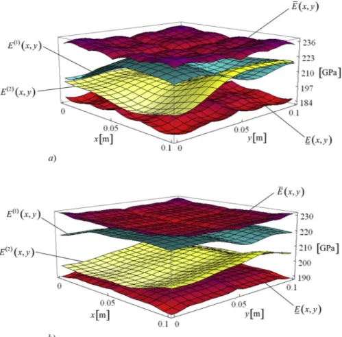
Fig. 3. LB, UB and two typical samples, E(1)(x,y) and E(2)(x,y), of the interval Young's modulus field over the plate domain for C
this aim, numerical methods proposed within a probabilistic framework for the solution of the Fredholm integralequation (5)with arbitrary integral kernel over non-rectangular domains may be adopted (see e.g. [44–47]).
It is worth mentioning that the proposed approach is also able to analyze problems involving multi-interval fields. In the present study, for the sake of simplicity, only Young's modulus of the material is assumed to be uncertain. Additional uncertain properties described as interval
fields, such as Poisson's ratio, can be incorporated into the FE
for-mulation by coding suitable User Subroutines. This would imply an increase of the dimensionality of uncertainty which can be handled by the proposed propagation strategy with reasonable computational costs.
Finally, it is observed that the non-intrusive implementation pre-sented in the paper can be readily extended to the case of uncertain properties modelled as random fields. Indeed, as outlined in Ref.[29], the interval field model based on the IIA via EUI is formally analogous to the classical KL expansion of a random field consisting of a super-position of deterministic spatial functions with corresponding random coefficients [42]. Within the probabilistic framework, a set of un-correlated standard random variables plays the same role of the EUIs. The propagation of random fields is more time consuming than the one of interval fields, especially when higher-order response statistics are desired. The probabilistic characterization of the response may be carried out by using the proposed ratio of polynomial response surface in conjunction with Monte Carlo simulation[24]. As known, however, the computational efficiency of sampling-based procedures rapidly worsens as the truncation order of the KL expansion increases since samples of a large number of random variables need to be generated. Conversely, the bounds of the interval response can be efficiently evaluated even for large truncation orders M of the KL-like decomposition of the interval
field.
Fig. 4. Bounds of the interval nodal displacements in the load direction of the
plate under uniform traction: comparison between the estimates provided by the proposed method and the vertex method for lB= L, a) CB= 0.05 and b) CB= 0.1.
Fig. 5. Coefficient of interval uncertainty of the nodal displacements in the load
direction of the plate under uniform traction: comparison between the esti-mates provided by the proposed method and the vertex method for lB= L, and two values of CB, namely CB= 0.05 and CB= 0.1.
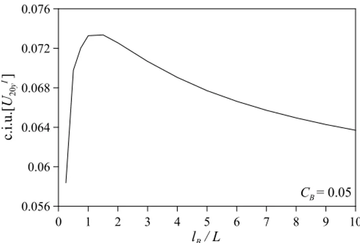
Fig. 6. Proposed coefficient of interval uncertainty of the displacement of node 20
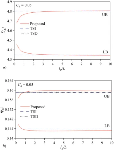
in the load direction of the plate under uniform traction versus the ratio lB/L (CB= 0.05).
Fig. 7. Bounds of the interval displacement of node 20 in the load direction of
the plate under uniform traction versus the ratio lB/L (CB= 0.05): comparison between the proposed estimates and the ones obtained under the assumption of TSI and TSD of the interval Young's modulus.
5. Numerical applications
The proposed IFEM implemented in ABAQUS is applied to analyze two square plates under different loading and boundary conditions. In both cases, the constitutive behaviour of the material is assumed to be linear-elastic isotropic with uncertain Young's modulus modelled as an
interval field based on the IIA (seeEq. (7)), i.e.:
= + = + = E x yI( , ) E [1 B x yI( , )] E 1 ( , ) ^x y e i M i i iI 0 0 1 (42)
where x and y are the Cartesian coordinates of a generic point of the 2D domain of the plates.
The spatial dependency function (seeEq. (3)) characterizing the
in-terval field EI(x,y) inEq. (42) is assumed to have the following ex-ponential form: = x y C x l y l ( , ; , ) exp B B Bx By 2 (43) where (x,y) and (ξ,η) are the Cartesian coordinates of two different points of the 2D domain. The parameter CBmay be regarded as the non-probabilistic counterpart to the standard deviation in random field theory[6], since it affects the deviation amplitude of the interval field
and thus the degree of uncertainty. Similarly, lBxand lBymay be viewed as the analogue of the correlation lengths since they rule the spatial dependency of the uncertain property along the x- and y-directions. Without loss of generality, it is herein assumed that lBx= lBy= lB. No-tice that, if lB→ ∞, the spatial dependency function in Eq. (43) ap-proaches the valueCB2, and the dimensionless interval function BI(x,y) in
Eq. (42) reduces to a symmetric interval variable, i.e.
=
B x yI( , ) bI be^Iwith deviation amplitude b = C
B. This circumstance implies the TSD of the uncertain Young's modulus which, indeed, turns out to be described by a single interval variable over the whole domain i.e.E x yI( , ) EI=E0(1+be^ )I. At the opposite extreme, as l
B→ 0, the TSI of the uncertain material property is achieved. In this case, Young's moduli of the FEs of the selected mesh are described by independent interval variables (see e.g.,[23,24]).
It is worth mentioning that, for regular domains, such as those employed in the square plates analyzed here, the eigenvalues and ei-genfunctions of the exponential function inEq. (43)can be evaluated in analytical form[42].
The accuracy of the proposed IFEM is assessed by performing ap-propriate comparisons with the bounds of the response provided by the
vertex method, which requires 2Mdeterministic analyses, M being the truncation order of the KL-like expansion of the uncertain Young's modulus inEq. (42).
Fig. 8. Samples of the interval Young's modulus (CB= 0.05, lB= L) which yield the a) LB and b) UB of the interval displacement along the y − direction of node 20 of the plate under uniform traction.
5.1. Plate under uniform traction with interval Young's modulus
The first application concerns a typical plane stress problem, i.e. a square plate clamped along one edge and subjected to a uniformly distributed traction along the opposite edge (Fig. 1). The material is assumed to have uncertain Young's modulus described by the interval
field inEq. (42). The following data are considered: width and thickness of the plate L = 0.1 m and t = 0.001 m, respectively; nominal Young's modulus E0= 210 GPa; Poisson's ratio ν = 0.3; traction p = 10 MPa.
The plate is discretized into N = 16 plane stress four-node elements. A complete Gauss quadrature integration rule is adopted. The interval nodal displacements in the load direction,UjyI, (j = 1, 2, ..., 20), are selected as response quantities of interest.
Both UMAT and USDFLD subroutines have been coded to in-corporate the interval field representation of Young's modulus into the formulation.
The truncation order M of the KL-like decomposition is selected by analyzing the rate of convergence of the proposed response surface ap-proximation (seeEq. (27)). Specifically, attention is focused on the LB and UB of the interval displacement of node 20 in the load direction, UIy
20. InFig. 2, such bounds are plotted versus the truncation order M, for CB= 0.05 and different values of the parameter lB. By inspection of Fig. 2, it can be inferred that, as the parameter lBincreases, the series converges more quickly, so that a smaller number of terms is required to represent the response surface inEq. (27)and, therefore, the interval
Young's modulus inEq. (42). To ensure a reasonable trade-off between accuracy and computational efficiency, M = 10 terms are retained for all values of the parameter lBherein considered. Alternatively, the op-timal truncation order M may be selected referring to suitable error measures similar to those introduced in the literature for assessing the accuracy of the truncated KL expansion of random fields (see e.g., [44–46]). For instance, in view of the analogy between the parameter
CBinEq. (43)and the standard deviation, global error measures related to the variance of the random field may be translated to the interval
field. Furthermore, the number of series terms may be significantly
re-duced by modifying the exponentially decaying spatial dependency
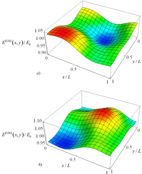
function to remove the non-differentiability at the origin[48]. In order to highlight the main features of the 2D interval field re-presenting the uncertain Young's modulus(42)over the plate domain, Fig. 3shows the LB function, E x y( , ), the UB function, E x y¯ ( , ), (seeEqs. (8a,b)), and two typical samples, E(1)(x,y) and E(2)(x,y), for C
B= 0.05 and two different values of the parameter lB, lB= 0.5L and lB= 5L. Specifically, the samples E(1)(x,y) and E(2)(x,y) are obtained from Eq. (7) setting e^iI=1,i=1, 3, 5, e^jI= 1,j i and
= =
e i
^iI 1, 1, 5, 7, 8, 10
,e^j =1,j i
I
, respectively. As expected, the results are enclosed by the LB and UB functions. Furthermore, it is observed that, as the value of the parameter lBincreases, the pattern of the interval field realizations consistently becomes more regular. Indeed, as already mentioned, when lB→ ∞, the interval field reduces to a single interval variable over the plate domain, that is the condition of TSD of the interval Young's modulus is approached.
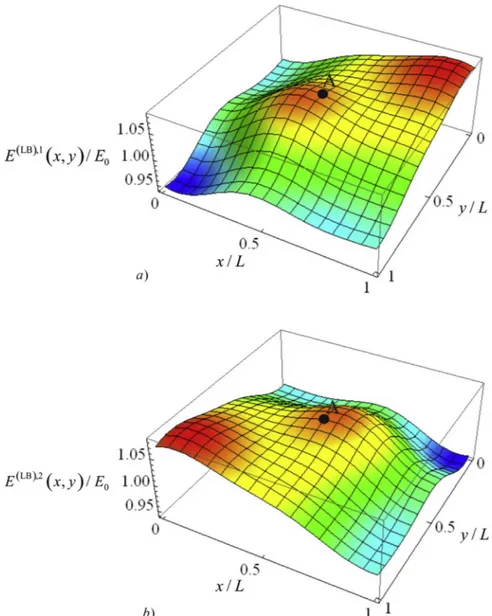
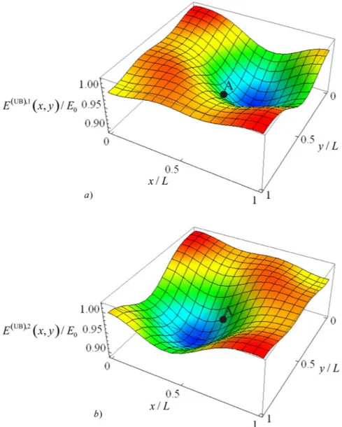
For validation purposes, the proposed bounds of the selected in-terval nodal displacements,UjyI, (j = 1, 2, ..., 20), are contrasted in Fig. 4with the ones obtained by means of the vertex method, for lB= L
Fig. 9. Contour plot of the displacement of the plate in the y − direction
cor-responding to the realizations of the interval Young's modulus which yield the a) LB and b) UB of the displacement in the y − direction of node 20, respec-tively (CB= 0.05, lB= L).
Fig. 10. Interval stress component in the load direction of the plate under
uniform traction evaluated at the integration points of a) FE 12 and b) FE 16: nominal value and bounds provided by the proposed method and the vertex method for lB= L and CB= 0.05.