Universit`a degli Studi di Pisa
Dipartimento di Informatica
Dottorato di Ricerca in Informatica
Thesis
: SSD (MAT/09 & INF/01)
Artificial Intelligence Techniques for Automatic
Reformulation and Solution of Structured
Mathematical Models
Luis Perez Sanchez
Supervisor Antonio Frangioni Referee Andreas Grothey Referee Tapio Westerlund
October 15, 2010
Largo Bruno Pontecorvo, 3 – 56127, Pisa, Italy email: [email protected]
Abstract
Complex, hierarchical, multi-scale industrial and natural systems generate increasingly large math-ematical models. Practitioners are usually able to formulate such models in their “natural” form; however, solving them often requires finding an appropriate reformulation to reveal structures in the model which make it possible to apply efficient, specialized approaches. The search for the “best” formulation of a given problem, the one which allows the application of the solution algo-rithm that best exploits the available computational resources, is currently a painstaking process which requires considerable work by highly skilled personnel. Experts in solution algorithms are re-quired for figuring out which (formulation, algorithm) pair is better used, considering issues like the appropriate selection of the several obscure algorithmic parameters that each solution methods has. This process is only going to get more complex, as current trends in computer technology dictate the necessity to develop complex parallel approaches capable of harnessing the power of thousands of processing units, thereby adding another layer of complexity in the form of the choice of the appropriate (parallel) architecture. All this renders the use of mathematical models exceedingly costly and difficult for many potentially fruitful applications. The i-dare environment, proposed in this Thesis, aims at devising a software system for automatizing the search for the best com-bination of (re)formulation, solution algorithm and its parameters (comprised the computational architecture), until now a firm domain of human intervention, to help practitioners bridging the gap between mathematical models cast in their natural form and existing solver systems. i-dare deals with deep and challenging issues, both from the theoretical and from an implementative viewpoint: 1) the development of a language that can be effectively used to formulate large-scale structured mathematical models and the reformulation rules that allow to transform a formulation into a different one; 2) a core subsystem capable of automatically reformulating the models and searching in the space of (formulations, algorithms, configurations) able to “the best” formulation of a given problem; 3) the design of a general interface for numerical solvers that is capable of accommodate and exploit structure information. To achieve these goals i-dare will propose a sound and articulated integration of different programming paradigms and techniques like, classic Object-Oriented programing and Artificial Intelligence (Declarative Programming, Frame-Logic, Higher-Order Logic, Machine Learning). By tackling these challenges, i-dare may have profound, lasting and disruptive effects on many facets of the development and deployment of mathematical models and the corresponding solution algorithms.
Acknowledgments
I would like to thank all the people that, in one way or another, helped me to walk across this beautiful and sometimes steep road. In particular, infinite thanks to my supervisor Antonio Fran-gioni. Without his patience, understanding and clarifying ideas, the realization of this work would have been impossible.
Thanks to Giorgio Levi for suggesting me to apply for the PhD in the first place and encouraging and supporting me throughout all the process. Thanks to Pierpaolo Degano and Ilaria Fierro, for an excellent PhD school organization and for giving us (foreign PhD students) full support during all these three years. Thanks to Giorgio Gallo for the crucial advices at each stage of the Thesis. Thanks to Andrea Maggiolo, Fabrizio Luccio and Linda Pagli for all the help and support since the very beginning.
Thanks to Luciano Garcia Garrido for introducing me to the Logic and Artificial Intelligence and for always motivating me to explore new and interdisciplinary points of view.
Thanks to Leo Liberti for the discussions regarding the experiments that helped me to build the methodology applied in this Thesis.
Thanks to Basuki, Flavio and Jorge for being three excellent PhD colleagues and friends and for all the moments together that made this experience a really nice one. Thanks to Sara, Fabrizio, and Sergio for the “intense” Bowling competitions. Thanks to Cristina and Daniela for always being caring friends even when we barely knew each other.
Vorrei inoltre ringraziare il Furnari, la Roglia, il Cataldi e il resto del team Torino, per uno spet-tacolare Bertinoro e per tutti bei momenti che abbiamo passato insieme. Grazie a Sara Capecchi per essere stata sempre dalla nostra parte e averci sempre appoggiato.
Grazie al team Cuneo: Chiara, Damiano, Elisa, Seutta, Valeria, Luca, Anna e Diego, per avermi accettato sempre come parte del gruppo, per le tante chiacchierate (anche quando io parlavo sempre in inglese). Grazie a mia “cognata” Mara, per la compagnia e l’amicizia, ma soprattutto per le grasse risate. Grazie a Danila e Diego per essere diventati dei fratelli per me, per le tante serate a giocare a domino mentre si ascoltavano le selezioni musicali da YouTube, e per tutti i preziosi momenti insieme.
Grazie a Carla e Gra per essere dei suoceri meravigliosi, per avermi accolto nella loro famiglia come un figlio, per tutto il supporto e la comprensione, e per i meravigliosi piatti che mi avete fatto assaggiare.
Gracias al Luisda, Pabli, Kmilo, Batista, Jose Carlos, Tomy, Mija, por todos los valiosos mo-mentos, desde las noches en el cub´ıculo 3 del C5, hasta las clases en la UH, las inolvidables sesiones en UH-SIS y podr´ıa seguir adelante.
Gracias a mi hermanita Thaizel por la important´ısima compa˜n´ıa durante todo este tiempo en Pisa, fundamentalmente durante el dif´ıcil inicio.
A los mejores padres que un hijo pueda desear, gracias a los dos por haberme apoyado siempre en mis decisiones, a´un cuando eran decisiones dif´ıciles. Gracias por todos los utiles consejos y por todo el amor que me han dado siempre. Por supuesto gracias tambien a la super abuela Zenaida por todo su cari˜no (y espectaculares garbanzos).
Contents
Introduction i
I.1 Modeling and solving with structures – Motivations . . . ii
I.2 The proposal and further motivations . . . iii
I.3 i-dare– Overview . . . . vii
I.4 Thesis structure . . . ix
1 i-dare(lib) – the structure library 1 1.1 Basic components . . . 1
1.1.1 Parameter Types . . . 2
1.2 Structure Classes . . . 2
1.2.1 Leaf Problem Class . . . 3
1.2.2 Block Class . . . 6
1.2.3 Block - Formal definitions . . . 7
1.3 Some Structure Class examples . . . 10
1.4 Discussion . . . 12
2 i-dare(im) – base modeling environment 13 2.1 Dimensions . . . 13
2.1.1 Local dimensions . . . 13
2.2 Variables and Constants . . . 14
2.2.1 Bounding . . . 15
2.2.2 Property well-formedness . . . 15
2.2.3 Indexing . . . 16
2.2.4 Expressions . . . 17
2.3 Scalars and Vectors . . . 20
2.4 Leaf Problem . . . 23
2.4.1 Local Leaf Problems . . . 24
2.5 Blocks . . . 26
2.6 Formulation . . . 29
2.7 Discussion . . . 31
3 i-dare(ei) – the enhanced instance 33 3.1 Instance Wrapper (IW) . . . 33
3.1.1 Global Data . . . 34
3.1.2 Data handler (DH) . . . 36
3.1.3 IW - Data Validation . . . 40
3.1.4 IW - Access methods . . . 41
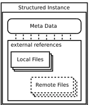
3.2 Structured Instance Generation . . . 42
3.2.1 Meta Data File . . . 42
4 i-dare(solve) – solving the model 49
4.1 Structured Modeling and Solving Methods . . . 49
4.1.1 Some initial formulation . . . 49
4.1.2 Knapsack constraints . . . 50
4.1.3 Logical Formula . . . 54
4.1.4 Disjunctive Scheduling . . . 54
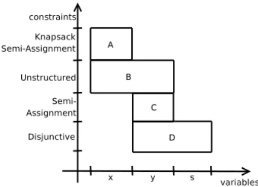
4.1.5 Product Loading . . . 55
4.2 Shared Variables – Blocks – Relaxation . . . 58
4.2.1 Returning to the Product Loading problem . . . 59
4.2.2 Tackling the other formulations . . . 60
4.3 Solvers’ Tree . . . 61
4.4 Solvers and Structures . . . 63
4.4.1 Solvers exported and new Structure relations . . . 65
4.4.2 Configuration Templates . . . 67
4.4.3 Solution Generation . . . 69
4.4.4 The overall solution process . . . 69
5 i-dare(t) - the reformulation system 71 5.1 Atomic Reformulation Rules . . . 71
5.1.1 Abstract structure classes . . . 72
5.1.2 Track Structures . . . 73
5.2 Algebraic ARR . . . 74
5.2.1 ARRP– Index declarations . . . 75
5.2.2 ARRP– Dimension relations . . . 76
5.2.3 ARRP– Mappings . . . 76
5.2.4 ARRP– Fixed template items . . . 80
5.2.5 ARRP– Conditional expression . . . 80
5.2.6 ARRP– examples . . . 81
5.2.7 Semantics . . . 83
5.3 Algorithmic ARR . . . 87
5.3.1 Semantics . . . 88
5.4 Selection domain and Reformulation Domain . . . 90
5.5 Discussion . . . 91
6 i-dare(control) - best (Formulation, Solver, Configuration) 93 6.1 Search Spaces . . . 93
6.1.1 Extended Model . . . 94
6.1.2 Solvers and Configurations . . . 94
6.2 Controlling the Search in the (Formulation, Solver, Configuration) Space . . . 94
6.2.1 Objective function computation . . . 95
6.2.2 Training and Meta-Learning . . . 99
6.2.3 The overall search process . . . 99
6.3 Experiments . . . 100
6.3.1 Further experimentation . . . 102
6.4 Discussion . . . 103
7 Combining structures and reformulations 105 7.1 Structures . . . 105 7.1.1 Compositions . . . 107 7.2 Creating a model . . . 108 7.3 Reformulations . . . 109 7.3.1 ProdBC to MILP . . . 110 7.3.2 SAbs to Composition . . . 111 7.3.3 VAbs to LP . . . 111
0.0. CONTENTS 9 7.3.4 SemiContinuous to MILP . . . 112 7.3.5 ProdCC to MILP . . . 114 7.3.6 SemiAssign to MILP . . . 114 7.3.7 Constraint to MILP . . . 115 7.3.8 OFMin to MILP . . . 115 7.3.9 IndComposition to MILP . . . 116 7.3.10 Composition to MILP . . . 117
7.4 Applying the ARRPs to HCP . . . 119
8 More focused structures and reformulations 123 8.1 Rounding Up previously defined structures . . . 123
8.1.1 Reformulations . . . 124
8.1.2 Reformulation Diagram . . . 129
8.2 Some Convex Structures . . . 130
8.2.1 Reformulations . . . 132 8.3 Quadratic Variants . . . 136 8.3.1 Reformulations . . . 137 8.3.2 Final diagram . . . 140 Conclusions 143 C.1 Perspectives on Deployment . . . 144 C.2 i-dare challenges . . . 146 Bibliography 149 A Frame Logic –FLORA-2 159 A.1 FL Syntax . . . 159
A.1.1 Alphabet . . . 159
A.1.2 Terms . . . 160
A.1.3 Formulas . . . 160
List of Figures
I.1 Schematic diagram of the full I-DARE system . . . vii
1.1 i-dare(lib) hierarchy . . . . 3
2.1 K-Vector examples . . . 21
2.2 Replication inside blocks . . . 27
2.3 An example of wrong component tree . . . 29
3.1 Structured Instance . . . 42
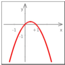
4.1 Representation of y(1-y) function . . . 50
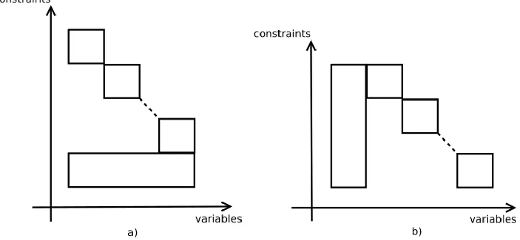
4.2 a) Shared variables partitioned over substructures (except for one) in a linear model b) Variables shared by all substructures in a linear model . . . 58
4.3 Graphic relating constraints with variables for formulation §4.1.5 . . . 59
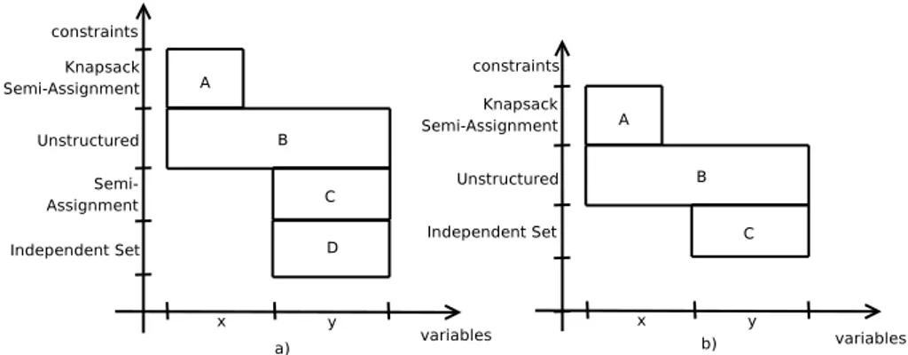
4.4 Graphic relating constraints with variables for formulation a) §4.1.5 and b) §4.1.5 . 61 4.5 Solver Tree assignment . . . 62
4.6 Formulation Diagram . . . 62
4.7 C++ vs. FLORA-2 hierarchies . . . 64
4.8 Overall solution process . . . 70
5.1 ARRPreformulation and solving process . . . 86
5.2 Formulation example . . . 90
6.1 GMLS diagram . . . 100
7.1 HCP Formulation . . . 110
7.2 Independent Composition of N MILP subproblems . . . 116
7.3 Composition of two MILP subproblems with shared variables . . . 118
8.1 Initial set of ARRs and structures . . . 130
8.2 Convex Structures and Reformulations . . . 136
Listings
1.1 Component Class . . . 2
1.2 Leaf-Problem class . . . 3
1.3 Leaf-Problem class example . . . 4
1.4 Another Leaf-Problem class example . . . 4
1.5 Yet another Leaf-Problem class example . . . 4
1.6 MCF class . . . 5
1.7 Local Leaf-Problem class example . . . 6
1.8 Block class . . . 6
1.9 Block class example . . . 7
1.10 Another block class example . . . 7
1.11 MILP block class modification (d loc) . . . 8
1.12 Simple Selection LfP class . . . 10
1.13 MMCF(FC) class . . . 10
1.14 Lagrangian Relax class . . . 11
2.1 Example of dimensions . . . 13
2.2 Local dimension definition . . . 13
2.3 Example of local dimensions . . . 14
2.4 Another dimension . . . 14
2.5 Class of properties . . . 14
2.6 Example of variable . . . 14
2.7 Bounding example . . . 15
2.8 Dimensions and Constants in i-dare(im) . . . 16
2.9 Aggregator Class . . . 18
2.10 Example of aggregator general form . . . 19
2.11 Example of a specific aggregator . . . 19
2.12 LfP specification . . . 23
2.13 LfP example . . . 23
2.14 LfPL specification . . . 24
2.15 LfPL example . . . 25
2.16 Automatic property generation . . . 25
2.17 Automatic dimension and index generation . . . 25
2.18 Example of property and dimension generation . . . 25
2.19 Block definition . . . 26
2.20 LP and Integrality constraint . . . 27
2.21 MILP block instance . . . 27
2.22 Another block example . . . 28
2.23 MILP MPS LfPL class . . . 28
2.24 Formulation class . . . 29
2.25 Full formulation example . . . 30
3.1 Instance Wrapper . . . 33
3.2 XML global data format . . . 34
3.3 DH Class . . . 36
3.5 XML Data Handler Class . . . 37
3.6 IW example . . . 37
3.7 MPS Data Handler Class . . . 37
3.8 LEAF Node general form . . . 43
3.9 BLOCK Node general Form . . . 46
4.1 Solver Root Class . . . 63
4.2 Blueprint exported to the FLORA-2 file . . . 64
4.3 Example of solution hierarchy . . . 65
4.4 Extension of :: FLORA-2 operator . . . 67
4.5 Example of Integer parameter type . . . 67
4.6 Example of Double parameter type . . . 67
4.7 Example of Integer parameter type . . . 68
4.8 Example of Choice parameter type . . . 68
5.1 ARR class definition . . . 71
5.2 ARRPclass definition . . . 75
5.3 ARRPto reformulate MCF to LP . . . 81
5.4 MMCF FC class . . . 82
5.5 ARRPto reformulate MMCF FC to Lagrangian Flow Relaxation . . . 83
5.6 Writer class . . . 85
5.7 Delegation solver FLORA-2 class . . . 86
5.8 Generate the path tree . . . 88
5.9 ARRAclass definition . . . 88
6.1 Solver Wrapper Interface . . . 96
6.2 Machine Learning Interface . . . 97
8.1 Continuous KnapSack Problem . . . 124
8.2 MILP to block MILP . . . 124
8.3 Branch and Bound block . . . 125
8.4 MILP to Branch and bound with LP . . . 125
8.5 Semi-Continuous MILP . . . 126
8.6 MILP-SC to MILP . . . 126
8.7 MMCF(FC) to MILP-SC . . . 127
8.8 Independent Replication Selection block . . . 129
8.9 MMCF(FC) to Lagrangian Knapsack Relaxation . . . 129
8.10 Quadratic Function . . . 130
8.11 Second Order Cone Program . . . 131
8.12 Mixed-Integer Second Order Cone Program . . . 131
8.13 MISOCP to Branch and bound with SOCP . . . 132
8.14 MIQP-SC-SEP to MISOCP . . . 134
8.15 Mixed-Integer Semi-Infinite Perspective Cuts (for the quadratic case) plus Linear Constraints . . . 135
8.16 MIQP-SC-SEP to MISIPC Q LC . . . 136
8.17 KnapSack Problem . . . 136
8.18 Quadratic Minimum Cost Flow . . . 137
8.19 QMCF to MCF through linearization . . . 138
8.20 QMMCF FC to Lagrangian Flow Relaxation . . . 138
Introduction
The development of mathematical models of reality, which often take the form of decision or op-timization problems, is arguably the single most important way in which humanity improves its understanding and control over the physical world. Coupled with the phenomenal growth of avail-able computational resources over the last 50 years, it has very substantially contributed to the exponential growth of knowledge in almost all scientific fields such as physics [109], statistics [81], data mining [86, 61], mathematics [105, 25], artificial intelligence [99, 44], and many others. Fur-thermore, countless many practical applications fundamentally hinge upon mathematical models in such diverse fields as transportation [29, 21], location [85, 107], scheduling [30, 90, 132], com-plex industrial systems [120], networks [28], bio-informatics [108], chemical engineering [23, 119], medical equipment configuration [116], and many others. Therefore, it is fundamental for the con-tinuous improvement of science and technology that better and better mathematical models, and the software packages required to solve them, be available to researchers of all fields.
However, it is one of the most striking and important discoveries of science and mathematics in the Twentieth Century that just being able of creating a model does not mean that there is a reasonable way to solve it. G¨oedel’s theorems [153], existence of non-computable functions [151], complexity theory [106], etc, have shown that being able to write a model is not equivalent to be able to solve it, i.e. for some models there may not be a way to compute a solution or doing it in a reasonable amount of time.
This impossibility was not clear, as testified by Hilbert in his Program [63]. Hilbert proposed to define a formulation of mathematics based on a solid and complete logical fundantion, believ-ing that this could be done by (1) showbeliev-ing that all mathematics follows from a correctly chosen finite axiom system; (2) and that such axiom system is provably consistent through means such as epsilon calculus [126]. It was Hilbert’s understanding that, once realized this, every possible problem in mathematics and science could have been solved by “just computing”. This dream was put to end initially by G¨oedel, who proved that any non-contradictory formal system, which was comprehensive enough to include at least arithmetic, cannot demonstrate its completeness by way of its own axioms (any effectively generated theory capable of expressing elementary arithmetic cannot be both consistent and complete).
G¨oedel’s results were later complemented by studies in computer theory (Turing [151], Von Neumann [155]), showing the existence of undecidable problems and non-computable functions, which of course make a model not solvable. Further down the same line, the existence of effectively computable functions, for which, can be shown that any algorithm that computes them will be very inefficient, in the sense that the running time increases exponentially (or even superexponentially) with the length of the input, which also makes the model not solvable (in a reasonable time) was discovered. Furthermore, currently, a huge number of decision and optimization problems (NP-Hard, NP-Complete) are believed to be unsolvable in polynomial time, although no formal proof is yet available (see [118, 100]).
Undeterred by the impossibility of a universal solution procedure (efficient enough), the scien-tific community has continued building better and better models. Since the “super-solver” is not available, each problem needs to be addressed individually, focusing in exploiting particularities
in their models. These particularities can be called structures, that are well known parts of a model for which exist particular solving techniques. Typically, problems can only be solved with algorithms that recognize and exploit these structures.
I.1
Modeling and solving with structures – Motivations
When a model of a practical industrial/scientific application is built, oftentimes a choice is made a priori (and possibly unintentionally) about which structure of the model is the most prominent from the algorithmic viewpoint. This is done by choosing first which of the several main classes of models the problem is molded in: a Linear Program (LP) [57], a Mixed Integer Linear Program (MILP) [127], and so on. This decision is mostly driven by the previous expertise of the modeler, by the“bag of tricks” she has available, and by her understanding (or lack thereof) of the intricate relationships between the choices made during the modeling phase and the effectiveness/availabil-ity of the corresponding solution procedures.
Unfortunately, making “the best” choice is arguably difficult. Many classes of models have been devised which are useful for expressing different practical problems, and the continuous improve-ments of solution methods have created an enormous wealth of results about different algorithmic approaches for (old and new) model classes and the conditions under which any approach is more or less computationally effective. For instance, Conic and Semidefinite Programs [31] allow for carefully selected forms of nonlinearities which keep the problems convex, and therefore efficiently solvable by appropriate classes of algorithms; they have many applications e.g. in engineering and computational mathematics, as well as having been the foundation of Robust Optimization where uncertainty of problem’s data is taken into account [32].
To further enlarge the set of representable functions while still guaranteeing efficient resolv-ability, Disciplined Convex Programming [82, 41] require problems to be specified by following a rigorous set of rules which ensure convexity, as well as providing solution algorithms with the data they need to effectively tackle the problem. While nonconvex problems are in general much harder to solve, an enormous number of variants arise according to the specific properties of the objective function and constraints that can be exploited for algorithmic purposes. Considerable attention has recently been devoted to nonconvex nonlinear problems, with [39, 88, 144] or without [117] integrality constraints on the variables.
Several special cases of particular interest arise when nonlinearities and/or nonconvexities are a consequence of expressing specific situations, such as: the optimization of a different objec-tive function by a different decisor [24, 68] or, more in general, the equilibrium between a set of different decisors [104]; constraints about joint probability of uncertain events to occur [43]; con-vex constraints with just one single concave component [95, 37], differential equation constraints [110, 131], and many others. Complex combinatorial structures, e.g. like the ones appearing in scheduling problems [90], can be embedded as “primitives of the modeling language” in Constraint Logic Programing (CLP) techniques [121, 22, 34] under the form specialized domain propagation techniques. And the list goes on and on.
When a model class has (more or less arbitrarily) been selected and the model has been writ-ten, a specific numerical solver has to be used to actually solve it. The typical choice is to rely on battle-hardened general-purpose solvers, capable of tackling (in principle) any one problem in the given model class without much intervention from the end-user. Unfortunately, general-purpose solvers may exhibit poor performance on many applications since they typically ignore any existing underlying structure. For each of the above problem classes, an enormous literature is available about techniques that are effective for solving specific sub-classes of problems; these include (to name just a few) preconditioning techniques in linear algebra [51, 74, 70], effective domain re-duction techniques [64] and hybrid search/optimization methods in CLP [65, 93], specialized row-and column-generation algorithms in MILP [30, 33, 59, 69, 77, 92], specialized search strategies in heuristic approaches [87, 44, 73, 85], appropriate selection and breeding procedures in evolu-tionary programs [80], and effective learning rules in swarm-intelligence approaches [60]. Thus,
I.2. THE PROPOSAL AND FURTHER MOTIVATIONS iii
for countless applications, specialized solvers exist that are better than general-purpose ones. Yet, because they are specific to smaller classes of problems, they are often much less developed, and therefore less robust and user-friendly, than general-purpose ones. In addition, their efficiency may crucially depend on the appropriate setting of some algorithmic parameters which requires a level of understanding of their inner workings that cannot be reasonably expected outside a small circle of specialists. On top of all this, practical problems most often exhibit several structures simul-taneously; not only it is not a fortiori clear which of them is computationally more relevant, but also the most efficient approach may require exploiting them all. This would call for integrating several different specialized approaches, a task most often bordering the impossible in the current state of affairs.
Thus, the fact that the most appropriate (specialized) approach is actually selected crucially depends on the realization of a long list of conditions: the user has to discover the structures (which requires knowing about them in the first place), realize that they are computationally relevant, fetch specialized numerical solvers capable of exploiting them, write the model fighting with the rigidities and quirks of the interface of the specialized solvers (such as requiring specific programming languages, using badly conceived input data formats, not allowing certain operations required by the applications, . . . ) and the inevitable configuration problems, and integrate all this in the environment required by the application. Often, modelers lack both knowledge and resources to perform these complex tasks; therefore the wealth of available knowledge about specialized algorithms for specific structures lies unused gathering dust in the uncharted backwaters of the scientific literature and/or in prototypical software codes which, despite holding great promises, are too specialized to be known and used outside a small circle of interested specialists. Meanwhile, end-users cannot solve their problem efficiently enough.
To make matters worse, computationally exploiting “the right” form of structure crucially depends on having chosen “the right” formulation that reveals it. However, many structures are typically not “naturally” present in the mathematical models, and must be purposely created by such weird tricks of the trade such as creating apparently unnecessary copies of variables and/or relations [84], replacing an exact compact nonlinear formulation with a much larger approximate linear one [142], replacing a single integer-valued variable by a set of binary-valued ones [69], and many similar others. That is, one needs a reformulation of the problem—which may well turn out to be rather different from the “natural” one familiar to the original modeler—where structures inside the model are transformed into other equivalent ones that are better suited to some carefully selected algorithmic approach. Finding these reformulations, and the corresponding algorithms with their appropriate configurations, is a costly and painstaking process, up to now firmly in the hands of very specialized experts—most often themselves blissfully unaware of the many potential practical applications of the techniques they master—with little to no support from modeling tools.
I.2
The proposal and further motivations
This Thesis will be focused in the proposal of a system, named i-dare (Intelligence-Driven Auto-matic Reformulation Engine), that defines the methodology necessary to deal with the problem-atics issued in the previous section: structured modeling, ((re)formulation, solver, configuration) selection, structured solver application.
From the foundational viewpoint, the main aim of i-dare is to challenge the implicit assump-tion, underlying all mathematical modeling efforts, that devising an effective mathematical model can only be achieved by human creativity, and that computer tools have no role on it. There are, of course, sound theoretical and practical reasons to believe that human creativity will ever—or at least for a very long time—be a necessary component of any mathematical modeling exercise. How-ever, as for countless many other human activities before, the intervention of automated system has a huge potential to improve the efficiency and effectiveness of these efforts, ultimately allowing the human skills to concentrate on these parts that are still firmly out of reach of computer systems.
that while the term reformulation is ubiquitous in mathematics (e.g. [39, 82, 101, 117, 142, 144, 154] among the countless many others: a Google search on the term returns more than 600,000 hits), there are precious few formal definitions and theoretical characterizations of the concept. Among the few ones, some are limited to syntactic reformulations, i.e., those that can be obtained by application of algebraic rewriting rules to the elements of a given model [113]. These reformulations are capable of exploiting syntactical structure of the model, such as presence of particular algebraic terms in parts of its algebraic description [71, 117]. While being very relevant, these do not include all transformations that have shown to be of practical use.
Oftentimes, reformulations are based on nontrivial theorems which link the properties of two seemingly very different structures; some notable examples are the equivalent representations of a polyhedron in terms of extreme points and faces (which underpins a number of important ap-proaches such as decomposition methods, and has many relevant special cases such as the path formulation and the arc formulation of flows [18]) and the equivalence between the optimal solu-tion value of a convex problem and that of its dual (which is the basis of many results in robust optimization). These reformulations require a higher view of the concept of structure of a model, i.e., a semantic structure which considers the mathematical properties of the entire represented mathematical objects as opposed to these of small parts of their algebraic description; we therefore refer to them as semantic reformulations. Proper definitions of reformulation capable of capturing this concept are thin on the ground.
For instance, an attempt was made in [143] by demanding that a bijection exists between the feasible regions of the two models and that one objective function is obtained by applying a monotonic univariate function to the other, which are extremely strict conditions. A view based on complexity theory was proposed in [24], but since it requires a polynomial time mapping between the problems it already cuts off a number of well-known reformulation techniques where the mapping is pseudo-polynomial [69] or even exponential in theory [30, 59, 73], but quite effective in practice. Only recently a wider attempt at formalizing the definition of formulation has been done which covers several techniques such as reformulation based on the preservation of the optimality information, changes of variables, narrowing, approximation and relaxation [113, 114].
However, a general formal definition of reformulation is not enough for i-dare; the aim is to identify classes of reformulation rules for which automatic search in the formulation space is possible. In this sense, syntactic reformulations, being somewhat more limited in scope and akin to rewriting systems, may prove to have stronger properties that allow more efficient specialized search strategies. Yet, defining appropriate more general classes of semantic reformulations is also necessary in order for the system to be able to cover a large enough set of possible reformulations. This calls for an appropriate definition of “structure” that on one hand is general enough, and on the other hand allows for effective search in the reformulation space.
Another crucial requirement is the ability to predict with a sufficient degree of accuracy some performance metrics of a given solution approach (with a given set of algorithmic parameters) on a given instance of a model, without actually performing the computation. This is necessary as it will provide the “objective functions” of the search, and is clearly a very difficult task. There is a huge literature on both complexity analysis and experimental evaluation of algorithms, and the system will have to be conceived as to allow exploitation of any available result for each specific solver and model classes. However, the system will also require some general-purpose approach to cover all the cases where no useful results are known. This would call for the application of machine learning techniques to the prediction of algorithms performances, and possibly for the selection of a set of “good” algorithmic parameters, a promising avenue of research which appears to have just started to produce the first concrete results [49, 96]. Yet, all the attempts so far have focused on narrow classes of problems and approaches; what would set i-dare far apart from any other previous attempt are the sheer scale and heterogeneity of the set of approaches that have to be addressed, as well as the extension of the approach to cover the case of different formulations for the same model. Results showing that accurate prediction is indeed possible, with existing or newly devised approaches, for such a varied set of algorithms may substantially impact the practice of parameters selection in several applications.
I.2. THE PROPOSAL AND FURTHER MOTIVATIONS v
From the technological viewpoint, none of the currently available methodologies and tools for mathematical modeling provides all the functionalities envisioned and needed by i-dare:
1. A modeling language capable of representing semantic structures, providing the user with a rich set of constructs that permits a representation of the problem which is “natural” form and independently from the underlying solution methods.
2. A core system capable of automatically reformulating the models and a search mechanism in the space of (formulations, algorithms, configurations) that is capable of finding “the best” formulation of a given problem, intended as the one which, applying the selected algorithm with its selected configuration, provides the most efficient solution approach.
3. A general solver interface capable of integrating specialized solution approaches by making it possible for one solver to use others as sub- or co-solvers independently from their algorith-mic details; this calls for a structured instance description language which, unlike currently available ones, is flexible enough to allow passing all parts of the data of the instance to each different involved specialized solvers in the format it requires and supports.
While 2. is arguably the most innovative feature, the other two components are also crucial for the overall success of the system. Remarkably, the need for these is indeed felt in the modeling and numerical solver communities, as witnessed by the fact that they have been addressed to some extent in several existing software projects. Yet, each of these project has focussed on specific aspects of the problem, without addressing the whole (challenging) general issue.
Regarding need 1, standard algebraic modeling languages like AMPL [66] or GAMS [15] are completely “unstructured”: they offer no support to partitioning a model into sub-components with clearly defined interfaces that may be developed and modified separately from each other. While you can define subproblems and have each of them solved by a different solver, each sub-model lives in the same namespace, and changes in any of them may (unintentionally) bear changes in the others. Thus, first-generation algebraic languages can be likened to the first generation of computer languages like FORTRAN or Basic in this respect, and share the same weaknesses: developing and maintaining large and complex models, while possible, gets rapidly extremely difficult as the size increases. The need for more structured modeling languages is clearly felt in the community, and it has been addressed in several ways. One is to rely on an existing Object-Oriented Programming (OOP) language, in order to inherit its structured programming capabilities: this is for instance the case of FLOPC++ [4] (using C++), puLP [134] (using Python) and of the commercial OptimJ product [130] (using Java). While this may help, it does not introduce “natural” constructs specifically for modeling; besides, it requires knowledge of the host programming language. Similarly, CP-based approaches like G12 [76] “naturally” allow for some degree of structured modeling due to the partial extensibility of the CP language, but they ultimately remain tied to a specific modeling and solving paradigm—although hybrid CP/MILP approaches are possible in SCIP [16] and ILOG (now IBM) Concert [54]—and to the underlying programming language (C or C++). The need for providing structure directly at the algebraic modeling level is addressed e.g. by the RIMA project [136], and is especially felt in the context of what is often referred to as multidisciplinary design or multidisciplinary optimization, giving rise to projects like ASCEND [156] and pyMDO [122] (both using the OOP capabilities of Python). However, the aim of these projects is “only” to make it simpler for the user to come up with a correct model; once that is done, the formulation is “flattened up” and passed to a general-purpose solver.
The main proposal of i-dare in this respect is to move up a further step of the ladder of expressive power, devising a modeling system based on declarative languages like Prolog [129]. In particular, Frame-Logic systems [102] like FLORA-2 [159] allow to combine the expressive power of declarative languages with OOP components, providing tools of unparalleled effectiveness for reasoning about structures. This is clearly necessary to deal with semantic (non-syntactical) structures, since then reformulations are not limited to application of algebraic rewriting rules, but require the capability of checking logical conditions for the applicability of a given reformulation rule.
Since logic programming paradigms, while extremely powerful, are even less familiar to the vast majority of perspective users than OOP ones, this logic-based modeling language should not be the only choice for interfacing with the system proposed in this Thesis. Instead, its primary role will be that of an intermediate modeling language, used to drive the core search and reformulation capabilities of the system (cf. 2. above) but largely invisible both to end-users and to algorithms developers. For the former, a number of different existing front-end systems may be adapted to produce the required intermediate language representation of the model; this is for instance the case of ASCEND (which comes already equipped with a nice GUI component) or pyMDO, but also extensions to popular alternatives like GAMS and AMPL can be considered, a-la SML [53]. Back-end communication with algorithms will be obtained through a general solver interface and a structured instance format, discussed next.
In order to work as planned, the system i-dare, requires a unified interface for “every possible solver”. The primary component of such an interface will have to be a(n extensible) structured instance format. File formats for solvers are often awkward remnants of the punched-cards era such as MPS [97], rather difficult to understand for all but the most technically-savvy users [140], and/or extremely fragmented so that the same model can be represented in several different incompatible ways [125] to suit the needs of the different available solvers. This makes it more difficult to collect instances of models for testing and validation purposes, requiring substantial work for the trivial and uninspiring task of converting one (awkward) data format into another. A unified data format with good expressive capabilities, thanks to the flexibility of XML, has been recently proposed in the Optimization Services project [137], extending the concept to that of data stream, e.g. served by a network connection. While the OS format may provide a convenient starting point, it will be necessary to extend it to explicit support for semantic structures, where some parts of the model are represented in “abstract” terms by providing indication of the intended semantic of the model rather than some algebraic description of its constraints. A logic and very convenient consequence of this choice is that the instance format should not be intended to replace every existing specialized data format, but rather to be a meta-format which, other than allowing to “natively” represent the data and the algebraic structures of the instance, may delegate the task of representing specific instance blocks (corresponding to specialized structures) to specialized data formats. This has several advantages, apart from that of not wasting resources re-inventing the wheel (for instance, the native format itself may be delegated to Optimization Services). It will be possible to use existing solvers with their natively supported data formats, without the need for an interface layer for a new language. Existing instances sets will not need to be translated in the new format, which may be error-prone and may increase their size (the flexibility of XML being often dearly paid in terms of size bloat) w.r.t. that of possibly highly compact specialized encoding. The data format will evolve together with, and adapt to, the set of supported solvers. Finally, the reformulation machinery of the core system will yield a universal data format translator, capable of automatically perform the conversion between any two sets of specialized formats for any two classes of models for which a (chain of) reformulation rule(s) exists in the system.
The universal data format will serve as basic input structure for a universal solver interface. The need for isolating the user from the details and quirks of the underlying solution methods is heavily felt, as demonstrated e.g. by the Open Solver Interface project [123] and the Stochastic Modeling Interface [12], both in COIN-OR [1], and by the MCFClass project [124]. Yet, these are limited to very specific classes of solvers and models. The traditional approach to the solver independence problem has been that of delegating the interface to the (algebraic) modeling language such as GAMS or AMPL; however, this is only possible when the underlying solver is a monolithic, general-purpose one.
The aim of the Thesis in this matter is to allow different solvers for specialized problems to be used together; therefore, a mechanism for generic solver collaboration will have to be devised and perfected. It is well-known that a trade-off between generality, efficiency and flexibility exists so that a mechanism devised for covering all potential uses is unlikely to be possible, or at least efficient enough. As for the structured instance format, the idea is therefore that of exploiting the semantic information embedded in the structured model description to allow solvers for a
I.3. I-DARE – OVERVIEW vii
given structure to impose constraints on the set of functionalities provided by other solvers they collaborate with, thus rendering the universal solver interface flexible and capable of incorporating existing interfaces like the previously mentioned ones.
I.3
i-dare
– Overview
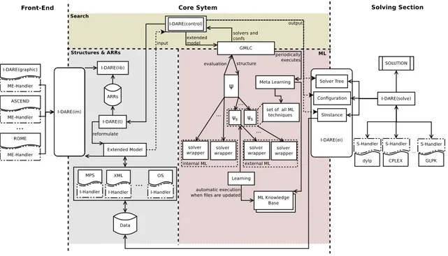
Figure I.1 provides a schematic description of the i-dare system. The system is divided into three main parts: front-end, core system and solving section, clearly separated by interfaces.
Figure I.1: Schematic diagram of the full I-DARE system
The front-end part will comprise one or more graphical and/or textual front-ends for the sys-tem. A general Modeling Environment Handler (ME-Handler ) must be designed that declares all functionalities that i-dare exposes to each modeling environment, effectively setting the interface between the front-end and the core system. The interface will rely on i-dare(im), the i-dare logic-based intermediate modeling language. Defining the ME-Handler, will not be considered as a part of this Thesis, whereas a detailed definition of i-dare(im) will be provided.
The core system is further subdivided in three parts: formulation and reformulation, perfor-mance evaluation, and control.
• The formulation part (denoted as “Structures and ARRs” in Figure I.1) is responsible for the definition of the structured model and of the corresponding structured instance, together with the set of reformulation rules that can be used to perform reformulations. It is based on i-dare(im), and composed by three modules. i-dare(lib) is the package containing all the structures that i-dare knows, together with the basic mechanisms to reason about formulations, such as verifying their well-formedness. When a formulation is complemented with a set of actual data it becomes an Extended Model (instance in standard optimization parlance); a general Instance Handler (I-Handler ) will be defined, which allows data to be retrieved from the different sources (files, databases, network connections, . . . ) using newly defined and/or existing data formats (cf. i-dare(ei)). A general deduction system, denoted as i-dare(t) will then be used to reformulate EMs by using the database ARR of Atomic
Reformulation Rules, together with the necessary argument (input) and answer (output) mappings between the two concerned structures. While most ARR could conceivably be directly applied to models, they are in general applied to EM for two reasons. The first is that applicability (or exact form) of a reformulation may depend on the actual data of an instance. The second is that gauging the computational impact of a reformulation cannot typically be done without some access to the actual data; this is in fact the rationale for the next component.
• The performance evaluation part (denoted as “ML” in Figure I.1) is responsible for the del-icate task of predicting the performances of each tentative reformulation, so as to compute the “objective function” which guides the search (itself governed by the next component). While it is clear that the performance evaluation will require some form of machine learning, it is fundamental to decouple the basic structure of the system from the details of the spe-cific learning method employed. Therefore, the ML approach will be “seen” by the control mechanism as a “black box”, described by an abstract General Machine Learning Control GMLC interface. Internally, a similar interface (denoted as Ψ in the figure) will be defined to allow any general ML approach to be used to actually perform the prediction. Some no-table details of the system, evidenced in the figure, require further comments. First, since a “solver” may actually be composed by a combination of several different solvers, each one will possibly have a different ML approach (denoted by ΨS in the figure). Second, given
the generality of the system, prediction will necessarily have to be solver-specific, with each solver at least extracting its tailored set of “features” from the instance and presenting them to the ML; this is the task of solver wrappers, that will have to be implemented to hook any numerical solver to the system. Third, while any solver will be able to rely on the “external” general-purpose ML approach, some solvers may have the capability of self-predicting their performances, either using highly tailored ML approaches or completely different techniques like complexity analysis. This “internal” ML will have to be appropriately presented to the general mechanism, e.g. to be used to compute the performance of the “overall” solver from these of its “sub-solvers”. Other crucial components of this part of the i-dare system are the actual continuous Learning mechanism which—either exploiting actual runs by end-users or using spare CPU cycles to perform test runs—updates the knowledge base upon which the prediction is performed, and the Meta Learning mechanism that allows to evaluate and compare different ML techniques for computing the Ψ function, thereby selecting those which provide the best results.
• Finally, the control part is composed by the package i-dare(control), in charge of guiding the search for the best (reformulation, solver, configuration) (f, s, c) triplet. In order to decouple the basic structure of the system from the details of the search mechanism—the appropriate choice of which will require substantial research—the package defines the abstract interface that any control mechanism will have available to guide the deduction process of the i-dare(t) package for generating the tentative reformulations, whose performances will be predicted by the GMLC component, until the desired (f, s, c) triplet is reached.
Finally, the solving section is responsible for actually performing the solution approach on the chosen (re)formulation, collecting and presenting the result to the core system, which will in turn refactor them in the format of the original instance to present them to the front-end. Its interface with the core system is the i-dare’s Enhanced Instance format i-dare(ei), itself composed by the three (f, s, c) parts:
• SInstance is the actual encoding of the final instance, obtained at the end of the reformulation process, represented in the structured instance format;
• Solver Tree is the description of the (set of) numerical solver(s) that has(have) been selected by the search process as the most appropriate for the given SInstance; as previously men-tioned, this is not just a solver but, in general, a structured collection of solvers, some of which using others to cope with specialized structures;
I.4. THESIS STRUCTURE ix
• Configuration is the description of the configuration(s) that has(have) been selected by the search process as the most appropriate for (each solver in) the Solver Tree and the given SInstance.
The i-dare(solve) package will then have to orchestrate the actual solution process, possibly taking into account issues like distributed computation, relying on the available set of Solver Handlers (S-Handler ), i.e., implementations of the general solver interface that allows to plug specific solvers to the i-dare system.
I.4
Thesis structure
This Thesis is be divided in an Introduction, eight Chapters and the Conclusions. This subdivision will provide the reader with a definition step by step of all modules in i-dare. Chapter 1, describes how structure classes and their relations can be created and stored, by defining the i-dare(lib) module. Chapter 2 defines the internal modeling language i-dare(im), formally describing all concepts of well-formedness, from the dimensions and indexes, to leaf problems, blocks and formu-lations. Chapter 3, specifies how the data can be attached to the formulations, by using the proper format handlers and wrappers; concluding with the definition of the structured instance. Chapter 4, describes how solvers can be attached to i-dare, and how they can be configured and linked to the structured instance, by means of a Solvers’ Tree. In chapter 5 we define all the necessary theory related with reformulations; we describe the concept of Atomic Reformulation Rules (ARR), how i-dare will treat them semantically, and how they can be applied to a formulation to define the Reformulations’ Domain. Chapter 6 describes the i-dare(control) module; it will describe the available search spaces and how can they be used to search for the “best” triple (formulation, solver, configuration). In Chapter 7 we declare a set of “simple” structure classes’ examples that will allow (by composition) the creation of complex models, and using these classes we will define some reformulations in order to obtain a MILP (or LP) structure. Whereas, in Chapter 8 we will focus on a set of structures for which there are specialized solution methods, and we will study how we can relate them by applying the appropriate reformulation rules. Finally the conclusions will sum up the results obtained and will describe the potentials and future research.
Chapter 1
i-dare
(lib)
– the structure library
Abstract
i-dare allows the construction of models based on an extensible structure class library. This structure class library contains a set of basic components that enables the definition of new classes of structures and how these classes will interact between each other. Components of i-dare(lib) will be included inside a hierarchy, abstracting the main characteristics of each structure class. Furthermore, this hierarchy enables the user, by adding new pieces, to enlarge i-dare(lib)’s potential. This chapter defines i-dare(lib) in a bottom-up fashion, starting from the most basic components like dimensions and parameters types, advancing to atomic problems and ending with problems compositions (blocks). At the end of this chapter some detailed examples are presented, together with a discussion about the usage of declarative programming (in particular FLORA-2 – cf. Appendix A) to define i-dare(lib).
1.1
Basic components
Every structure class is ultimately reduced to a set of parameters (plus the semantical meaning of the structure class). The parameters represent the characteristics of the input and output of the structure class. For example, let’s examine a LP structure class:
min/max X i civi s.t. X i c′
j,ivi ≤ / = / ≥ bj for all j
To create an “instance” of the LP structure class, we need to specify the direction (min or max), the vector in the objective function, the matrix in the constraints, the right hand side vector, the relation that will be used in each constraint and the vector of variables on which the solution will be stored. Moreover, we need to know how the cardinalities of the previous elements are related to each other. Observe that the number of objective function constants must correspond to the number of variables and the number columns in the constraint matrix. These cardinalities will be called dimensions (see §2.1). For instance the previous LP structure class has two dimensions, that can be called columns and rows.
Definition 1.1.1 (Dimension Meta Variable (dMV)) To define how many dimensions a struc-ture class will have, i-dare(lib) will use the propertydim var−>[d1, . . . , dk], where k is the number
of dimensions, and diand dj are identifiers, such that di6= dj, ∀i, j ∈ [1..k]. Each di will be called
dimension Meta Variable (dMV) and it represents a set [0..kdik − 1]. kdik states for the dimension
For the LP structure class the dMV list may be,dim var −> [cols, rows].
1.1.1
Parameter Types
As mentioned previously, parameters are a key element in the definition of a structure class, therefore when defining a structure class in i-dare(lib) we must be able to specify the types of potential parameters. These potential parameter types can be,
• d var– Variable type • d constant– Constant type
• d vector(?K,?S)– Vector type • d rel – Relation type • d direction – Direction type
Variable and Constant Types (d var and d constant)
These two types are used to denote the variables and constants of the structure class respec-tively. For instance, in the previous LP structure class example, xi is of variable type and ci is of
constant type. Formal definition on well-formed variables and constants will be given in §2.3. Vector Type (d vector (?K, ?S))
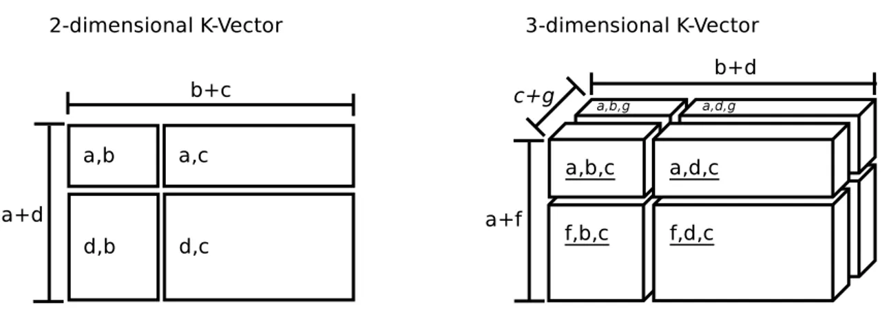
When we use dimensions while defining constants, variables, relations or even general expres-sions a vector may be produced. The vector type is denoted using d vector(?K, ?S), where ?K ∈ {
d var, d constant, d rel } and ?S must be a non-empty list of dMVs. |?S| represents the number of dimensions of the vector (e.g. a matrix is a 2-dimensional vector).
For instance,d vector(d constant, [ cols ])represents a one dimensional vector of constants. On the other hand, when {d vector(d constant, [ cols ]), d vector(d var , [ cols ])} appear in the same parameter list (of a certain structure), it indicates that the number of elements of the first and second vector are the same. Well-formed vectors will be formally defined in §2.3.
Relation Type (d rel)
Another kind of argument is the relation, denoted using d rel. Relations allowed by i-dare will be binary over R × R, like, = (equality), =< (less than or equal) and >= (grater than or equal). Direction Type (d direction)
There are structure class that may contain an objective function within them. In this case, the structure class may require the specification of objective function’s direction as one of its parame-ters. Supported directions areminandmax. Although both directions are transformable multiplying the objective function by −1, we decided to keep them both for the sake of expressibility.
1.2
Structure Classes
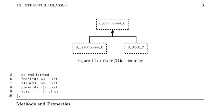
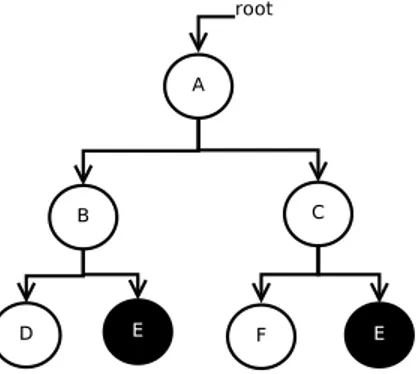
i-dare(lib) defines a basic hierarchy for the structure classes that one may create. This hierarchy is composed of three classes,d Component C, d LeafProblem Candd Block C(see figure 1.1).
The most general structure class (d Component C) will define the most general behaviors that
every other structure class must implement. This class is defined as follows, Listing 1.1: Component Class
1 d Component C [
2 a b s t r a c t , 3
1.2. STRUCTURE CLASSES 3
d_Component_C
d_LeafProblem_C d_Block_C
Figure 1.1: i-dare(lib) hierarchy
5 => w e l l f o r m e d , 6 f r e e i n d s => l i s t , 7 a l l i n d s => l i s t , 8 p u r e i n d s => l i s t , 9 v a r s => l i s t 10 ] .
Methods and Properties
• wellformed– tells whether a component is well-formed or not. • vars – retrieves the list of variables used within a component. • freeinds – retrieves the list of free indices of a component.
• pureinds– retrieves the list of all indices used as constants within expressions in the component. • allinds – retrieves the list of all indices used within the component.
In the declaration ofd Component Cappears a class boolean field, namedabstract. When this field
appears in a class definition the system will not allow the creation of instances from that class. The definition of the d Component C class introduces for the first time the concept of index. Indices will be formally defined in §2.2.3, but let’s give at least an empirical definition that may be useful in the rest of the chapter.
An index is an identifier linked to a dimension (and used to iterate over that dimension). For instance, xi from the LP example, uses the index i that iterates over dimension cols. The free
indices of a component in i-dare are the set of indices that are not fixed by any construct like vectors or cumulative operators likeP. For example if we use the constant c′
ij (with indices i, j)
which appears insideP
ic′ij then j would be a possible free index (if not fixed elsewhere).
All methods ind Component Care inherited and/or overwritten by all its descendant classes.
1.2.1
Leaf Problem Class
As a special case of component, i-dare(lib) defines the class of leaf problems. A leaf problem is an atomic definition composed of at least an objective function or a constraint. For example, linear problems, disjunctive constraints and quadratic objective functions are leaf problems. Henceforth leaf problems will be called LfP.
All LfPs must inherit from the following class,
Listing 1.2: Leaf-Problem class
1 d L e a f P r o b l e m C : : d Component C 2 [ 3 a b s t r a c t , 4 [ l o c a l ] 5 6 // Methods and P r o p e r t i e s 7 d i m v a r => l i s t , 8 [ di m bo und => l i s t , ] 9 a r g s => l i s t 10 ] .
Methods and Properties
• dim var– defines the list of dMVs of the LfP.
• dim bound– specifies which constants will have as domain a dMV’s set of values. optional
• args – defines the parameter types that the LfP will require.
The list of argumentsargs must be defined as a dictionary [name = parameter type ...], wherename
is an identifier unique inside the LfP.
A simple example of LfP would be the class of integer problems, Listing 1.3: Leaf-Problem class example
1 d I C C : : d L e a f P r o b l e m C 2 [ 3 d i m v a r −> [ d ] , 4 a r g s −> [ 5 i v a r = d v e c t o r ( d v a r , [ d ] ) // v a r i a b l e s t o be i n t e g e r 6 ] 7 ] .
This class will define the problems having a set of integer variables (ie. ivari ∈ Z,i ∈ d). As another
example, one can define the class of linear constraints with its list of argument types. Listing 1.4: Another Leaf-Problem class example
1 d L i n e a r C o n s t r a i n t s C : : d L e a f P r o b l e m C 2 [ 3 d i m v a r −> [ d1 , d2 ] , 4 a r g s −> [ 5 x = d v e c t o r ( d v a r , [ d1 ] ) , // v a r i a b l e s 6 A = d v e c t o r ( d c o n s t a n t , [ d2 , d1 ] ) , // A m a t r i x 7 b = d v e c t o r ( d c o n s t a n t , [ d2 ] ) , // b v e c t o r 8 r e l s = d v e c t o r ( d r e l , [ d2 ] ) // r e l a t i o n s f o r e a c h c o n s t r a i n t 9 ] 10 ] .
The LfP d Linear Constraints C represents all constraints with the formP
iAj,ixi relj bj ∀(j). We
may also define the class of linear problems (LP),
Listing 1.5: Yet another Leaf-Problem class example
1 d LP C : : d L e a f P r o b l e m C 2 [ 3 d i m v a r −> [ c o l s , c o n s ] , 4 a r g s −> [ 5 x = d v e c t o r ( d v a r , [ c o l s ] ) , // v a r i a b l e s 6 c = d v e c t o r ( d c o n s t a n t , [ c o l s ] ) , // p r i c e c o n s t a n t s 7 A = d v e c t o r ( d c o n s t a n t , [ c o ns , c o l s ] ) , // A m a t r i x 8 b = d v e c t o r ( d c o n s t a n t , [ c o n s ] ) , // b v e c t o r 9 r e l s = d v e c t o r ( d r e l , [ c o n s ] ) , // r e l a t i o n s f o r e a c h c o n s t r a i n t 10 d i r = d d i r e c t i o n // o b j e c t i v e f u n c t i o n d i r e c t i o n 11 ] 12 ] .
Note that in this case we are defining a complete LP with objective function and constraints. Once we use the parameter type d direction we are giving a hint that within that component there must
be an objective function. This leaf problem is represented algebraically in the following way,
dir X i cixi s.t. X i Aj,ixi relj bj ∀(j)
1.2. STRUCTURE CLASSES 5
Looking at LfP’s properties we find one that has not been previously defined, the dim bound. This property declares which constant parameter (vector or not) must have a domain restricted by a dMV. Thedim boundlist must have the following form: [( CN,D ),...], whereargs [CN]=d constant
ord vector(d constant, ? ), andD∈dim var. This property essentially constraints the parameterCNto take values between 0 and kDk − 1.
The next example will be a Minimum Cost Flow LfP (MCF). For this LfP we used the classical graph representation and we wrote it into i-dare(lib) syntax. This example will illustrate the usage ofdim bound
Listing 1.6: MCF class 1 d MCF C : : d L e a f P r o b l e m C 2 [ 3 d i m v a r −> [ N, E ] , 4 a r g s −> [ 5 SN = d v e c t o r ( d c o n s t a n t , [ E ] ) , // s t a r t n o d e s 6 EN = d v e c t o r ( d c o n s t a n t , [ E ] ) , // end n o d e s 7 SD = d v e c t o r ( d c o n s t a n t , [ N ] ) , // s u p p l y / demand 8 c o s t = d v e c t o r ( d c o n s t a n t , [ E ] ) , // c o s t p e r a r c 9 u = d v e c t o r ( d c o n s t a n t , [ E ] ) , // a r c c a p a c i t y 10 f l o w = d v e c t o r ( d v a r , [ E ] ) // f l o w v a r i a b l e s 11 ] , 12 di m bo und −> [ ( SN , N) , (EN , N ) ] 13 ] .
We used two dMVs, one to represent the nodes (N) and the other to represent the arcs (E). Using those dMVs we created a set of parameters, to represent:
• the arcs with SNandEN, so each arc will be <SNi,ENi>,i∈ [0..|E| − 1];
• the supply/demand of each node, supply implies a positive value, demand a negative one, otherwise must be 0 (SD);
• the the cost and the capacity of each arc (cost andu); • the flow variables (output of the structure) (flow).
Note that the SN and EN parameters must have values between 0 and kNk − 1; in fact they are restricted by thedim boundproperty.
A MCF may be also represented using a LP. If we define N+(i) = {j | (i, j) ∈E} and N−(i) =
{j | (j, i) ∈E}, representing the outgoing and incoming arcs, respectively, then
min X (i,j)∈E costijflowij s.t. X j∈N+(i) flowij− X j∈N−(i) flowij=SDi i ∈N 0 ≤flowij≤uij (i, j) ∈E
Using this LP formulation we may apply any LP solution approach to solve it. However, explicitly recognizing MCF as a structure class, allow us to apply specific solution approaches, like:
• Cycle Canceling: a general primal method [103];
• Minimum Mean Cycle Canceling: a simple strongly polynomial algorithm [78].
• Successive Shortest Path and Capacity Scaling: dual methods, which can be viewed as the generalizations of the Ford-Fulkerson algorithm [62].
• Cost Scaling: a primal-dual approach, which can be viewed as the generalization of the push-relabel algorithm [79].
• Network Simplex: a specialized version of the linear programming simplex method [124]. These algorithms have proved to be more efficient for several types of graphs, with respect to the plain LP approach.
Local Leaf Problem Class
In the LfP class definition we specified an optional property local. When this property is present it indicates that the potential instances will define all their data in a particular local format (e.g. MPS, OSiL, DIMACS, etc). A LfP class that contains the property local will be called Local Leaf Problem (LfPL) Class. An example of LfPL class may be,
Listing 1.7: Local Leaf-Problem class example
1 d LP MPS C : : d L e a f P r o b l e m C 2 [ 3 d i m v a r −> [ c o l s , c o n s ] , 4 a r g s −> [ 5 x = d v e c t o r ( d v a r , [ c o l s ] ) , // v a r i a b l e s 6 c = d v e c t o r ( d c o n s t a n t , [ c o l s ] ) , // p r i c e c o n s t a n t s 7 A = d v e c t o r ( d c o n s t a n t , [ c o ns , c o l s ] ) , // A m a t r i x 8 b = d v e c t o r ( d c o n s t a n t , [ c o n s ] ) , // b m a t r i x 9 r e l s = d v e c t o r ( d r e l , [ c o n s ] ) , // r e l a t i o n s f o r e a c h c o n s t r a i n t 10 d i r = d d i r e c t i o n // o b j e c t i v e f u n c t i o n d i r e c t i o n 11 ] , 12 l o c a l 13 ] .
d LP MPS C represents a class of LPs that takes all data from MPS format files. The parameter
types in the case of LfPL classes represent what data the LfPL will export to be used globally. At least variables should always be present in the parameter type list, otherwise there will be no communication between the LfPLand the rest of the model. In any case, it is always advisable to include the maximum possible set of parameter types, due to problem reformulation requirements (see §5).
1.2.2
Block Class
Problems can be built from the composition of other subproblems. For instance, e MILP problem can be seen as the composition of a LP and integer constraints. These compositions, will be called, blocks. Every block must inherit from the following class.
Listing 1.8: Block class
1 d B l o c k C : : d Component C [ 2 a b s t r a c t , 3 4 // Methods 5 i d s => l i s t , 6 s ubs C => l i s t , 7 l i n k => l i s t , 8 [ r p l R => l i s t ] 9 ] . Methods
• ids – represents a list of identifiers, one for each substructure class. • subsC– is the list of substructure classes.
1.2. STRUCTURE CLASSES 7
• rplR– is an optional field that represents a list of elements of the form?id = ?dt, where?id ∈ ids
and?dtmust be an algebraic expression involving the following operands, – a termA(d), whereA ∈ idsandd ∈ A.dim var; or
– a template item (c.f. Definition 1.2.6).
The substructure classes will represent the structures that are grouped by this block, and the
link represents how the variables inside those structures will interact with each other (see §1.2.3 for formal definitions).
Here is an example to illustrate how a block could be constructed: Listing 1.9: Block class example
1 d B MILP C : : d B l o c k C 2 [ 3 i d s −> [ l p , i c ] , 4 s ubs C −> [ d LP C , d I C C ] , 5 l i n k −> [ [ X , Y ] , [ X ] ] 6 ] .
In this case we are defining the MILP class using a block construction. The first sub-structure is a LP class and the second one is an Integrality Constraint (IC) class. But how do we ensure that the set of variables to be integer is a subset of the variables in the LP sub-component? For doing that we use the link list.
A link is a template of the variables to be used in the substructure of a block. Each member of a link correspond to a substructure. For example, [X,Y]correspond tod LP Cand [X]to d IC C. In this case [X,Y]is telling us that the variables of its corresponding substructure have to be exported in two groups, the variables linked toXand the variables linked toY. But since there is a second element in link, [X], we need to ensure that the variables exported by d IC Cand the first group of
d LP Care the same.
There is a formal definition for link’s behavior, that can be seen in §1.2.3. The most important part of this definition is the Different Name Unification rule DNU, that ensures that the link unifies with the exported variables satisfying that equal templates must correspond to identical variable groups and different templates must correspond to variables groups with no element in common. The following example will illustrate this fact.
Listing 1.10: Another block class example
1 d B v a r d e p t C : : d B l o c k C
2 [
3 i d s −> [ m a s t e r , s l a v e ] ,
4 s ubs C −> [ d Component C , d Component C ] ,
5 l i n k −> [ [ X , V ] , [ X ,W] ]
6 ] .
In this case the first and second substructure class must export an identical group of variables for
X but must export groups of variables forV andW with no elements in common. In section §2.5, we will see more detailed examples of how the variables can be exported ensuring the DNU rule.
1.2.3
Block - Formal definitions
This section will introduce step by step all the elements that compose a block, defining them formally.
Definition 1.2.1 (Class item) Given?C::d Component C, then a class item can be defined as one of the following two terms:
1. ?C– represents one structure of class?Cfor which the system will try to assign a solver, 2. d loc (?C) – represents one structure of class?C for which the system will not try to assign a
When the system is trying to assign a solver to a block, and it encounters a class item of the form d loc (?C), it will completely ignore that substructure. The system will assume that the solver assigned to the container block will deal with that substructure.
For instance we could modify the d B MILP C example indicating that the d IC C structure will be treated inside the solver assigned tod B MILP C, using the d loc modifier.
Listing 1.11: MILP block class modification (d loc)
1 d B MILP C : : d B l o c k C 2 [ 3 i d s −> [ l p , i c ] , 4 s ubs C −> [ d LP C , d l o c ( d I C C ) ] , 5 l i n k −> [ [ X , Y ] , [ X ] ] 6 ] .
Using the previous definition we can define the subsC property of blocks, as a list of class items. On the other hand, the ids property must be a list of non-repeated identifier, such that |ids| = |subsC|.
While integrating several substructures together shared variables may occur. The following four definitions will focus on how variables can be exported from substructures.
Definition 1.2.2 (Variable Tuple) Let V be a set of variables, then a variable tuple of V is (v1, ...., vm), where 0 < m ≤ |V |, vi∈ V, i ∈ [1..m], vi6= vj, i 6= j ∈ [1..m]. If m = 1 the parenthesis
could be removed. The empty tuple will be represented by ().
For example if V = {v, w, x, y} then the following are variable tuples: • (),
• w, • (v, y), • (y, v) and • (w, y, x).
On the other hand, (w, y, w) is not a variable tuple, because the w is repeated. A permutation of a variable tuple generates a different one. For example, (v, y) and (y, v) are different variable tuples. Definition 1.2.3 (Disjoint Variable Tuples) Let vt and wt be two variable tuples of sets V and W , respectively, then vt and wt are disjoint if they do not contain common variables.
For instance, (v, x) and (w, y) are disjoint, whereas (v, y) and (w, y, x) are not, because they have y in common.
Then finally using variable tuples we will be able to construct lists of tuples that denote how the block will recognize the variables of its sub-structures.
Definition 1.2.4 (Variable Pattern) Let V be a set of variables, then a pattern over V , is a list L of variable tuples of V , such thatS|L|
i Li⊆ V and Li∩ Lj= ∅ for all i 6= j ∈ [1..|L|].
For example, the following are variable patterns: • [v, (x, y)],
• [(w, x), (y, v)]and • [v, y, w]
Also a permutation of the variable tuples inside a variable pattern generates a different one. For instance, [v, y, w]and [y, v, w]are different variable patterns.