Preliminary study for the assessment of discontinuity’s size through Machine Learning algorithms

(1)

ALMA MATER STUDIORUM

UNIVERSITÀ DI BOLOGNA

SCHOOL OF ENGINEERING

-Forlì Campus-

SECOND CYCLE MASTER’S DEGREE in

INGEGNERIA AEROSPAZIALE / AEROSPACE ENGINEERING

Class LM-20

GRADUATION THESIS

in Aerospace Structures

Preliminary study for the assessment of discontinuity’s

size through Machine Learning algorithms

CANDIDATE:

SUPERVISOR:

Matteo Sarti

Professor Enrico Troiani

CO-SUPERVISOR:

Professor Marcias Martinez

(2)

(3)

ACKNOWLEDGEMENTS:

First of all, I would like to thank my supervisor, Professor Enrico Troiani, as he put me in contact with Professor Martinez at Clarkson University1_{and, moreover, he always supported}

me during the choices on how to carry out this study.

To Professor Marcias Martinez goes all my gratitude for helping, guiding and advising me during this journey, and for letting me use his machine throughout the simulation’s period. Even if it was not possible to meet physically, the work we did together has been a source of great personal growth for me.

I would like also to thank Dr. Francesco Falcetelli, PhD student at the University of Bologna. Since he was one of the previous three students who went to Clarkson University1 to carry out his Master Thesis in Aerospace Engineering, I had some very profitable conversations with him and I first got to know the environment I would have eventually found. Moreover, since his current PhD is inherent to the Structural Health Monitoring field, we were able to constructively compare some different choices before putting them into practice within this study. He is a really nice and helpful person, and for this reason he has all my gratitude.

I would now like to thank, from the bottom of my heart, all my family: my parents Stefano and Barbara, my two dear grandmothers Luisa and Mirella, my aunt Patrizia, and the many other members of this great family. They always gave me their support, advising and encouraging me in every choice not only during these university years but since I was born.

Another great thanks goes to all my friends: the Squad, the companions of skiing adventures, family friends, bandmates, fellow tennis players, fellow students, and many others. I will not list you all herein, but you know who you are and that you are all really important to me. The genuine people I met throughout my life gave me something special, a stimulus for personal growth, and it is right that they are here remembered and properly thanked.

Last but not least, I think I have to thank myself too. I know, it may seem a little bit selfish, but I had to make many sacrifices to achieve these results in a faculty that is certainly very demanding, but is even more rewarding when you eventually get to the finish line and accomplish your goals on time.

(4)

ABSTRACT:

During the last two decades there has been a huge breakthrough in the Structural Health Monitoring field, especially in the study of Acoustic Emissions (AE), to get qualitative and quantitative damage-related information.

This thesis attempts to focus on the possibility of obtaining an automatic estimate of small discontinuity’s length in an aluminium plate, by analysing some impinging signals when they interfere with the defect itself. The novel aspect about this analysis is that it was conducted through “trained” classification and regression algorithms that have been able, up to some extent, to automatically classify and predict the desired responses. This means that Artificial Intelligence, in particular Machine Learning techniques, were employed and played an important role within either the identification and the predictive part of this study.

Due to the SARS-CoV-2 global pandemic, and the consequent closure of the US embassies, it was not possible to obtain the Visa and go to Clarkson University1 to perform the experimental campaign there. Therefore, in order to collect the raw signals for the subsequent analysis, a comparison between Abaqus CAETM and OnScaleTM software was firstly enforced, and eventually the latter was chosen to perform the whole set of numerical simulations exploiting a pitch-catch configuration.

___________________________________________________________________________ 1_{Clarkson University in Potsdam, 13699, NY, USA, is the university in which the co-supervisor of this thesis}

works and where the author was supposed to go. This thesis was indeed co-supervised by Professor Marcias Martinez, head of the HolSIP Laboratory at that university.

(5)

ABBREVIATIONS - ACRONYMS:

AE – Acoustic Emission AI – Artificial Intelligence

ANN – Artificial Neural Network(s) CBM – Condition-Based Maintenance CFL – Courant - Friedrichs - Lewy CNN – Convolutional Neural Network(s) CTOD – Crack Tip Opening Displacement FE – Finite Element

GCON – General CONnectivity (unstructured mesh) GLW – Guided Lamb Waves

GUI – Graphical User Interface NDE – Non Destructive Evaluations NDT – Non Destructive Testing PCA – Principal Component Analysis PLB – Pencil Lead Break

PoD – Probability of Detection

PWAS – Piezoelectric Wafer Active Sensor PZT – Piezoelectric lead Zirconate Titanate RMSE – Root Mean Square Error

SHM – Structural Health Monitoring STFT – Short Time Fourier Transform ToA – Time of Arrival

(6)

LIST OF FIGURES:

Figure 1.1: PoD curves for some NDE techniques . . . 4

Figure 2.1: SHM flowchart . . . 8

Figure 2.2: Structure lifetime vs. quality plot, with and without SHM . . . 9

Figure 2.3: Passive (a) vs. Active pitch-catch (b) and Active pulse-echo (c) techniques . 10

Figure 2.4: Amplitude and envelope of a modulated signal . . . 12

Figure 2.5: P, S and Rayleigh waves . . . 13

Figure 2.6: Symmetric and Anti-symmetric modes . . . 16

Figure 2.7: Dispersion curves of a 2 mm Al plate . . . 17

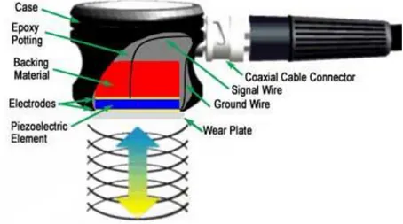
Figure 2.8: Scheme of a PZT transducer . . . 19

Figure 2.9: Example of an AE signal recorded by a PZT sensor . . . . 20

Figure 3.1: Cosine bell function . . . 25

Figure 3.2: Some features of a hit . . . 27

Figure 3.3: Three representation techniques of the same signal . . . . 30

Figure 3.4: Wavelet window across the time-frequency plane . . . . 34

Figure 3.5: Database creation sequence of the Shazam algorithm: (a) Spectrogram, (b) Constellation map, (c) Hash generation, (d) Hash details . 37

Figure 3.6: Map of hash pairs for a 15 seconds sample . . . 38

Figure 3.7: General working scheme of a pattern recognition algorithm . . . 38

Figure 3.8: Result of a clustering process . . . 40

Figure 3.9: Machine Learning algorithms . . . 42

Figure 3.10: Machine Learning workflow . . . 45

Figure 4.1: Comparison of window functions . . . 47

Figure 4.2: 5 cycle 600 kHz Hanning windowed tone burst . . . 48

Figure 4.3: Dispersion curves provided by the Vallen Systeme software for the 1.6mm A7075-T651 plate . . . 53

Figure 4.4: Oscillations at the end of the actuated 600 kHz Hanning window signal . 54

Figure 4.5: SRM subdivided area around the test piece . . . 58

Figure 4.6: Tie Constraint between plate and actuator . . . 58

Figure 4.7: 200 kHz S0 comparison between Abaqus CAE and OnScale . . . 59

Figure 4.8: Example of a standard mesh with the use of keypoints . . . . 61

(7)

Figure 4.10: Example of a model with keypoints along x and y axis . . . 62

Figure 4.11: A0 abnormal damping as the sim goes on . . . 63

Figure 4.12: Example of a 3D refined structured mesh . . . 64

Figure 4.13: Hybrid mesh and glued surfaces of the model . . . 65

Figure 4.14: A0 normal propagation (x, y and z velocity graphs) . . . . 66

Figure 4.15: Plate geometries . . . 67

Figure 4.16: Assigned loads . . . 68

Figure 4.17: Required values to model the damping behaviour . . . . 70

Figure 5.1: Sensors’ positions on the 3D model . . . 73

Figure 5.2: 2_5 and 10_90 at sensor 1: time domain (A), frequency domain (B) and spectrogram (C) . . 74-75 Figure 5.3: 2_5 and 10_90 at sensor 2: time domain (A), frequency domain (B) and spectrogram (C) . . 76-77 Figure 5.4: 2_5 and 10_90 at sensor 3: time domain (A), frequency domain (B) and spectrogram (C) . . 77-78 Figure 5.5: Elements of an amplitude vector . . . 80

Figure 5.6: Peaks extracted from an amplitude vector . . . 81

Figure 5.7: Elements extracted from an envelope vector . . . 82

Figure 5.8: Peaks extracted from an envelope vector . . . 82

Figure 5.9: Starting window for a new learning session . . . 84

Figure 5.10: Best Confusion Matrix for sensor 1 . . . 87

Figure 5.13: Best Confusion Matrix for the merged signals . . . . 89

Figure 5.14: Best predicted responses for sensor 1 . . . 92

Figure 5.17: Best predicted responses for the merged signals . . . . 93

(8)

LIST OF TABLES:

Table 3.1: Sensors coordinates and distance from the discontinuity . . . 22

Table 3.2: Full factorial design process . . . 23

Table 4.1: PZT 5A Navy II material properties . . . 51

Table 5.1: Correlation index between 2_5 and 10_90 . . . 74

Table 5.2: Classification’s results . . . 85-86

(9)

CHAPTER 1

1. ABOUT THE TOPIC

An acoustic emission (AE) signal is triggered by many phenomena occurring to the material such as, for example, crack initiation and growth. When a crack is present, the stress level at the crack tip is extremely high and therefore acoustic emissions are primarily emitted from the tip of a growing crack.

In general, it is possible to state that they originate from stresses and strains and some of the stronger acoustic emissions take place when a material is loaded either near / at / beyond its yield stress, therefore undergoing plastic deformation. Contemporarily, at microscopic level, the atomic planes slip and release energy in the form of elastic transient waves which then propagate through the material.

The more severe is the triggering event, the higher is the amount of energy released, and thus the amplitude of the generated waveform. This amplitude is also proportional to the crack propagation’s velocity: indeed, fast growing cracks would produce larger AE signals with respect to slow ones.

Once this signals are detected and converted into their digital counterpart, it is possible to exploit various AE testing techniques: a further analysis of these signals with specialized equipment may then lead to valuable qualitative and quantitative information regarding the crack features.

In the following section, the main issues related to damage characterization (in particular sizing) are stated. This will help defining how Machine Learning algorithms could be helpful in order to identify different outcoming signals associated to an input wave interfering with a discontinuity.

Experiments will also be required in a future development of this preliminary work to validate these results. This is mainly due to the simplifications that are introduced and explained throughout this thesis, of which the most relevant is for sure the presence of a signal interfering with a non-physical already present discontinuity of predetermined geometry, instead of proper modelled acoustic emissions associated with realistic crack propagation phenomena.

(12)

1.1. Damage characterization

Most of the existing methods using guided waves for damage characterization only focus on identifying its nature and position, but not its size [1]–[8]. The reason is that most of them exploit imaging reconstruction algorithms that do not provide accurate quantitative measures. Indeed, up to the very recent years, the damage growth has been mostly assessed exploiting either these kind of algorithms or damage indexes properly defined and processed to obtain a graphical reference of the growing crack. Recently, He et al. [9] attempted to understand whether two signal’s features (amplitude and phase change) may be exploited as crack length indicators; moreover they also questioned whether finite element (FE) simulations could replace experiments in gathering raw data in order to simplify the research activity and make it cheaper. The aim of this thesis is somehow related to these topics since the goal is to collect raw data by numerical simulations and evaluate if their features can be automatically recognized by Machine Learning algorithms, and related to the discontinuity’s size.

Su et al. proved that the active sensing, together with a diagnostic imaging algorithm based on linear and non-linear features of the acoustic waves, is effective in providing a quantitative estimation of the damage, ranging from microscopic flaws to macroscopic cracks [10].

Zhao et al. showed that strong attenuations and scattering of acoustic waves are present when dealing with characterization of complex and large geometries [11]. Instead, in this thesis it was considered a 1.6 mm thick plate with a rectangular geometry available in the HolSIP Laboratory at Clarkson University. This is due to the dispersion curves1 being already experimentally calculated for this thickness and material, and for possible future validation’s experimental activities.

In the same article, the crack growth is evaluated using a circular array of piezoelectric transducers2, however these techniques require a very detailed calibration and unfortunately need for a large array of transducers. Indeed, the methods utilizing piezoelectric transducers (called “active”) usually require a large number of sensible points and, sometimes, a baseline signal to be compared with the signal recorded on the damaged structure in order to have an accurate defect estimation. A novel example of a possible array configuration and signal processing technique to estimate the location and size of the damage is reported in [12], where the plate’s structure is divided in many cells.

Despite these drawbacks, scattering can be effectively exploited to characterize the damage’s ___________________________________________________________________________ 1_{Refer to figure 4.3 [13] to see them.}

(13)

size: as an example, Eremin et al. considered in [14] to use the scattering resonance frequencies of the acoustic wave to non-destructively estimate composite delamination, since these frequencies proved to be related to the crack’s variations of size and depth along its path. Pavelko stated in [15] that the opening and closing movements associated to the crack motion change the acoustic impedance of the material, hence they affect the propagation of the acoustic waves through it. Moreover, the fracture surface’s roughness and its local plastic deformation constitute other critical factors and obstacles for the propagation of elastic waves.

The crack itself also causes a partial reflection, hence a decrement of the wave energy, that could be used to assess the damage’s size. Therefore, it is also important to evaluate the position of the sensors on the structure in order to receive a distinguishable signal.

Giurgiutiu and Poddar stated in [16] that nowadays very few passive methods3_{exist to}

quantitatively identify the crack’s size, and this technique was actually the primary choice for this work if it would have been possible to access the laboratories to perform experimental collection of raw data. Since this was not the case due to the pandemic, in this thesis the simulations were performed exploiting an active method4 in a pitch-catch scenario. The motivations regarding the choice of this particular method are better explained in section 3.2. The reason why passive methods are rare may lie behind the fact that with active sensing the generated signals can have the amplitude the user prefers, even a very high one, which enables the sensors to detect the acoustic waves even for high scattering phenomena and in a noisy environment. On the other hand, when dealing with an acoustic emission generated directly from the growing crack, the amplitude might be very small, thus making the caption extremely complicated (pre-amplification is necessary).

Researchers like Bhuiyan et al. developed in [17] a novel technique of using piezoelectric transducers to detect low amplitude AE signals triggered by a fatigue crack, exploiting different sensors configurations in a passive way. Another example of a passive technique is the one exploiting local vibrational modes along the crack surfaces that may arise directly from the primarily tip-emitted acoustic waves interfering with the defect itself. Analysing this phenomena could help estimating the crack length as reported in [18].

___________________________________________________________________________ 3_{It is a method where there are no actuators involved, therefore the signal is recorded by sensors which are simply}

“listening” to the surrounding environment.

4_{It is a method where, on the contrary to the previous one, there are both actuators and sensors involved. The signal}

is defined by the user, sent to the actuator which excites the material, and eventually recorded by the sensors after a travelling period. To have a deeper insight about this distinction refer to section 2.1.

(14)

1.2. Scientific question

As already mentioned, acoustic waves propagating in a solid medium have been widely studied, especially throughout the last two decades, and many results have been found in terms of detection and localization of damages. However, these techniques are still under great research activity and are not employed in the industry because they are challenging to exploit when dealing with the whole structure of an aircraft.

The reason why these methods are not certified, and consequently used on large scale, is primarily related to the still high uncertainty and poor replicability of the results. This leads to the lack of a statistical model describing the effectiveness of the measuring technique, the so-called Probability of Detection (PoD) curves. Indeed, these graphs report the ratio between correctly detected defect and the whole defects present (i.e. a probability) on the ordinate, vs a defect parameter (e.g. length) on the abscissa. These curves are mandatory and needs to report values above a predefined threshold in order to be accepted by the certification authorities therefore, until they are properly defined, this kind of structural monitoring will remain a research topic.

Examining the chart reported in figure 1.1, it is possible to state that new Structural Health Monitoring (SHM) inspection techniques should be able to detect defects of 2 mm in length with a PoD of around 70-80% in order to be comparable with the other non-destructive evaluation (NDE) methods like penetrant liquids, radiography, ultrasonic testing and, mostly, eddy currents [19].

The latter are currently successfully employed to study cracks at early fracture stage, however the main requirements of a direct access to the structure and a point-by-point measure are great

(15)

limitations for these technologies. An alternative is therefore represented by SHM, especially through embedded Lamb wave techniques.

As a matter of fact, acoustic signals are unfortunately very susceptible to noise, vibrations and other disturbing phenomena (such as external loads, temperature, humidity, and even the geometry and boundary conditions themselves) that can significantly alter the captured signal. For this reason, thresholds settings, implemented by proper filtering operations during the signal analysis, are extremely important; however, they tend to be set according to a specific case study, thus resulting in a not replicable hit detection law [20].

Another important aspect is that the damage, after being detected and localized, needs to be properly quantified and, as it was mentioned in section 1.1, this is still an ongoing matter in the engineering field, where many different techniques are being developed and tested.

This thesis wants indeed to deal with the problem of quantifying a damage exploiting acoustic signals, but it does that through a novel technique firstly used by N. Facciotto in his Master Thesis [21] who was inspired by the well known ShazamTM music recognition software. The idea constituting the foundations of this preliminary work is that each event is supposed to have its own fingerprint, which basically carries some features identifiable within that sole detected signal. These could then be exploited by Machine Learning algorithms able to automatically recognize and build relations between them in order to eventually, and hopefully, understand the related defect’s size.

The necessity of an automatic process, which is also quite novel in the damage quantification researches, is due to the increasing amount of data usually collected during these kind of studies that would lead to a complicated and time consuming human-based analysis.

Based on the aforementioned reasons, the scientific questions the author wants to answer are: - Are there features carrying quantitative information about the size of a small defect ? - If so, is there at least an algorithm able to effectively identify them ?

1.3. Thesis structure

This thesis is structured in several chapters and sections that allow the reader to properly understand the ideas behind this study and the developed path. The preliminary literature review

(16)

has been very useful, especially for better understanding the general scientific field this thesis is developing through, which is the Structural Health Monitoring (SHM), and the fundamental pillars of the wave propagation phenomena.

Chapter 1 provided an outline of the main challenges and questions this study is trying to answer, moreover it focused the attention on the present state of the art regarding the damage characterization techniques.

Chapter 2 presents the literature review regarding Structural Health Monitoring and elastic waves propagation (in particular Lamb waves) since the reader might be interested in knowing the general qualitative and mathematical features of this particular research field. Furthermore, a brief introduction about piezoelectricity and piezoelectric transducers is given.

Chapter 3 gives an overview of the subjects addressed in this study starting from the general methodology, going through the choice of an active pitch-catch configuration for the numerical simulations, main signal analysis’ methods, principal features of the ShazamTM algorithm and, eventually, the different Machine Learning techniques.

Chapter 4 comprises all the aspects related to the numerical simulation part of the thesis. In it, the input signal exploited, the selection of the PZT transducers, the excitation and sensing methods, the modelling software and parameters needed in order to get the proper output signal to be subsequently processed are reported. Moreover, a comprehensive comparison between two different commercial software (Abaqus CAETM and OnScaleTM) is presented.

In Chapter 5, the recorded time domain output signals are firstly pre-processed, examined and eventually processed to prepare them for the subsequent step. The signal analysis through the Machine Learning algorithms is also presented, together with the best results.

Chapter 6 deals with the final considerations and conclusions. The future works necessary to develop what has been presented in this preliminary study are also addressed herein.

Eventually, all the articles, books and websites consulted in the development of this thesis are listed in a detailed bibliography.

(17)

CHAPTER 2

2. INTRODUCTION

During the last few years, the leading companies of the aerospace commercial industry have been launching some new efficient aircraft models that significantly reduce the fuel consumption. This is achieved not only through the employment of new high by-pass ratio engines but also through lighter and stiffer structures allowing, at the same time, weight reduction and increment of passenger comfort. Two examples regarding this latter aspect could be the lower cabin altitude and larger windows present on the Boeing 787 Dreamliner.

The demand of lighter structures goes hand in hand with the necessity of keeping a very high safety level, and it is here that Structural Health Monitoring (SHM) may play an important role.

2.1. Structural Health Monitoring

A precise definition of SHM is given in [22] where it is stated: “The process of

implementing damage identification strategies for aerospace, civil and mechanical engineering infrastructure is referred to as Structural Health Monitoring”.

The techniques gathered inside this field are sometimes quite different, but they all aim at real time monitoring the health state of a structure continuously throughout its entire working period. This is in contrast with the current destructive methods, where external (i.e. non-embedded) devices are employed.

Some drawbacks linked to the employment of NDT&E techniques are [19]: - The necessity of a regular scheduled-based maintenance;

- Massive disassembling operations in order to provide access even to the smallest components that have to be inspected;

- Either the increased safety factors during the design phase or the need of reinforcements to ensure the safety of the operations in between successive inspections, where the damage may grow unpredictably fast or defects may go undetected.

This weight increment restricts the performances, reduces the payload and raises the fuel burnt, consequently leading to an augmentation of the operational costs and of the environmental pollution.

(18)

The SHM steps can be divided as following [23]:

- Sensing, defined as the collection of the most adequate data from the monitored structure. For example, mechanical (e.g. surface displacement, stress, strain) or acoustic (e.g. impedance) properties can be recorded exploiting different types of commercially available sensors. An important aspect to take into account regards also the location and the number of sensors in order to control the most critical points of the structure, which have to be identified a priori by the designer.

- Diagnosis, defined as the extraction of damage related features from the acquired data exploiting properly developed algorithms to understand, if a damage exists, where, what and how severe it is.

- Prognosis, defined as the assessment of the residual operational life of the structure through different methodologies, including the rapidly growing Artificial Intelligence (AI).

The more the prognosis is accurate the more it is possible to perform the so-called

condition-based maintenance (CBM) rather than the scheduled-based maintenance

(linked to the widely used damage tolerance design approach) decided by the manufacturer and mandatory after a certain amount of flight hours [24].

(19)

Referring to figure 2.1, the flowchart at the base of SHM is here better explained. First of all, the sensors receive a signal travelling on the monitored structure and send it to the structural health monitoring subsystem for its processing and consequent diagnosis. Meanwhile, the usage monitoring subsystem is performing its evaluation about the environmental conditions and the structure’s mechanical behaviour. Then, linking these information together through the merging of the two subsystems, the prognosis is provided. To perform this final task, the damage’s features must be known to the overall health management system.

What is described here is the so-called intelligent structure, that is actually the final result at which all the researchers in this field aim to come putting together all the discoveries made throughout the years.

Thanks to CBM, which is an integration to the current damage tolerance approach, there will be a time reduction of the maintenance layover since the airplane would be taken away from operations only when needed and not on mandatory scheduled dates. As a consequence also the maintenance cost would drop while the safety of the aircraft would be ensured by systems constantly checking the health state of the structure throughout its life span.

The real time checking of a structure through embedded transducers could lead to a better exploitation of the materials at disposal, together with an increment of the structural safety: indeed, if the SHM system detects a damage prior to the scheduled inspection, the airplane can be properly fixed prior to its scheduled date. This cutting-edge technology may also replace some of the rigid inspection protocols enforced to reduce the probability of human error.

(20)

There exist a lot of SHM methods, but it is possible to group them in two broad classes highlighted in figure 2.3 [23]:

- Passive techniques are defined as the methods exploiting only sensors to “listen” to any change in the structure. These signals are recorded and analysed through specific algorithms in order to evaluate the structural health state.

- Active techniques are instead defined as the methods exploiting actuators sending a signal onto the structure (excitation phase), and properly placed sensors recording the dynamic response, that is later processed. Baseline data representing the damage-free scenario are sometimes needed in order to compare the damaged and the pristine system’s dynamic responses.

(21)

Modern SHM systems consist of a network of transducers incorporating active and passive techniques, i.e. Guided Lamb Waves (GLW) and Acoustic Emission (AE).

AE is one of the most recent and promising technique and is properly a passive method for the monitoring of structures because, as already mentioned at the beginning of Chapter 1, the emission source is located at the damage site and its nature can be very different: crack opening, plastic deformation, friction, impacts, delamination, matrix cracking and fiber rupture are all AE sources generating peculiar broadband signals that have to be properly monitored. Fiber optics, piezoelectric and strain sensors are some examples of sensors exploited in the passive techniques.

The expression “acoustic emission” is, however, also used to indicate active methods in which an input signal defined by the user is triggered into the material leading to the propagation of elastic waves. If the material is bounded by two surfaces (e.g. in a plate) it is more correct to name the emission as “guided waves”. GLW are commonly studied as an active technique for damage detection. Pencil Lead Break (PLB), Ultrasonic probes, Piezoelectric and Laser actuators are some examples of triggering techniques.

2.2. Elastic waves

The acoustic waves propagating in a solid material are related to the particles vibrational motion around their equilibrium position caused by elastic displacement and restoration internal forces [58].

According to the direction of the particle’s speed vector, these waves can be grouped in two broad classes moving with different phase velocities:

- Longitudinal waves are characterized by the same direction between the particle’s speed vector and the wave’s phase speed vector. They are also called “pressure waves” (P). - Transverse (Shear) waves are characterized by a particle’s speed vector and a wave’s

phase speed vector which are orthogonal. These can be encountered only in solid materials and are usually generated by extracting energy from the longitudinal waves.

To better understand the previous definitions it is important to state the difference between

group and phase velocity of a wave [59].

The wave’s phase velocity Cp is the one representing the rate at which the phase of a specific

(22)

necessarily coincide with the wave’s proper propagation velocity. The phase of a particular wave is expressed by a value ranging from 0 to 2π and it is taken at a certain time during the wave evolution. The phase velocity is defined by relations (2.1):

𝐶

_𝑝

=

𝜆

𝑇

= 𝜆 ∗ 𝑓 =

𝜔

𝑘 [m/sec] (2.1)

where λ is the wavelength [m], T is the wave period [sec], f is the wave frequency [Hz=1/sec],

ω=2πf=2π/T is the angular frequency [rad/sec], and k=2π/λ is the wavenumber [rad/m].

Waves usually encountered in the practical applications considered in this thesis are multifrequency, therefore a second velocity must be defined to have a complete understanding of the topic. This is the group velocity Cg, it represents the motion of the envelope, hence the

energy propagation through the material, and it is defined by equation (2.2):

𝐶

_𝑔

=

𝜕𝜔

𝜕𝑘 (2.2)

This velocity is exploited to assess the Time of Arrival (ToA) of a wave packet.

The envelope of a signal, highlighted in figure 2.4, is the curve tracing the signal amplitude peaks (it is the shape of a modulated wave). Therefore, the amplitude is an instantaneous value while the envelope is the curve formed by the peaks succession.

(23)

2.2.1. Lamb waves

When a solid material is unbounded, the acoustic waves propagating through it are referred to as bulk waves (since they propagate inside the bulk of the material) and they possess some universal properties. However, these waves can be encountered only for very thick components (where this dimension is much higher, theoretically infinite, with respect to the wavelength) and this is not the case for aerospace structures which are usually made of thin parts assembled together.

When an elastic material is bounded, the problem becomes more complex since new elastic surface waves arise simply due to the particular geometry of the component: it is the case of

Rayleigh (if the material is bounded by just one surface) and Lamb waves (when the bounding

surfaces are two, like in a plate) [60].

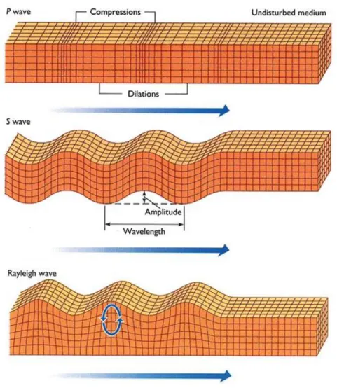
Rayleigh waves usually penetrate to a depth of one wavelength and their motion combines both longitudinal and transverse movements creating an elliptic particle path, as visible in the following figure:

(24)

As for Rayleigh waves, the Lamb waves particles’ motion is once again elliptical. The latter are the most common guided waves, meaning that the wave motion is guided by the two surfaces bounding the plate, and their name derives from the mathematician Horace Lamb who discovered and characterized them in an homogeneous, isotropic and infinite plate1 during the 1917 [25].

The derivation and explanation of their entire set of equations is out of this thesis’ scope, but interested readers can find useful information in reference [26].

What is important to mention is that there exists two families of wave modes (symmetrical and anti-symmetrical, about the plate’s mid-thickness plane) in infinite plates whereas, in unbounded medium, just the longitudinal and the transverse modes are present.

These latter surface waves are useful in NDE applications since they are very sensitive to many kind of defects and follow the surface’s geometry during their motion. For this reason, they can be used to inspect areas that other types of wave may not reach. Moreover, these waves possess a high susceptibility to any kind of interferences and this can be positive (e.g. in case of damage detection) or negative (e.g. in case of near boundaries and presence of noise) according to the purpose they are exploited for, which is usually the SHM.

Lamb waves have also the peculiar feature to travel long distances even in materials having high attenuation (like the ones having lots of inhomogeneities, e.g. CFRP) due to their high propagation’s velocity, this leads to the possibility of fast checking a large component without the need of a large amount of equipment [27].

However, this latter property brings to the problem regarding the examination of small components, where the reflections from the edges may become a huge source of signal distortion. The time interval for an acoustic wave to reflect around the test piece (thus leading to another hit detection by the sensor) ranges a lot depending on the damping properties of the material itself. This means that the temporal windows considered for the signal analysis are of crucial importance to get reasonable results and have to be carefully evaluated.

___________________________________________________________________________ 1_{In defining the problem, H. Lamb assumed a 2D scenario regarding the particles’ motion: they were restricted to}

the normal to the plane (z) direction and to the wave propagation (x) direction. Motion just along the y-direction was assigned to another set of modes, called shear-horizontal (SH).

This means that GLW and SH modes are complementary and, moreover, they are the only ones possessing the property of travelling with straight and infinite wave fronts along a plate.

(25)

As reported in section 2.1, researchers are trying to develop techniques based on the physical principles of Lamb waves in order to go from the qualitative indication of the occurrence of a damage to the final prediction of the structural residual life, passing through a quantitative assessment of the location and severity of the damage itself.

The merits associated to the inspection of a component through Guided Lamb Waves (GLW) can be resumed in [28]:

- The ability to inspect large structures during service (avoiding disassembling and retaining even the coating and the insulation) provided that the detection area is sufficiently small;

- The possibility of checking the entire cross section for a fairly long length; - The lack of complicated, expensive and movable devices during the inspection; - The good sensitivity to many different defects;

- The low energy consumption and great cost-effectiveness.

As mentioned, two main Lamb wave modes exist and each of these modes may be composed by multiple harmonics mainly due to the excitation frequency and plate thickness.

Their dispersive properties2 can be obtained by finding the solutions to the propagating Lamb waves equations. By applying the proper boundary conditions fulfilling the plate geometry requirements (i.e. zero stresses on the upper and lower surfaces), the following dispersion relations are found for, respectively, the longitudinal symmetric “extensional” and the transverse anti-symmetric “flexural” modes (depicted in figure 2.6).

tan(𝑞ℎ) tan(𝑝ℎ)

= −

4𝑘2𝑞𝑝 (𝑘2_−𝑞2₎2

(2.3) tan(𝑞ℎ) tan(𝑝ℎ)

= −

(𝑘2−𝑞2)2 4𝑘2_𝑞𝑝

(2.4) where: 𝑝2 ₌ 𝜔2 𝐶𝐿2− 𝑘 2_{and 𝑞}2 ₌ 𝜔2 𝐶𝑇2− 𝑘 2 _(2.5)

h is half of the plate thickness, k is the wavenumber, 𝜔 is the angular frequency,

(26)

For isotropic materials the longitudinal and transverse wave propagation’s velocities 𝐶𝐿 and 𝐶𝑇

can be expressed directly through the Young modulus E, the Shear modulus G (or the Poisson ratio μ) and the density ρ [61]. This means that each material has its own dispersion relations and curves. The reader can imagine how the problem’s complexity rises when anisotropic or orthotropic laminated materials are involved in the analysis.

Many examples of industrial tools for the experimental evaluation and plotting of the dispersion curves are available: the Vallen SystemeTM software exploited in [13] is one of them.

___________________________________________________________________________ 2_{By dispersive property is intended the relation between the wave propagation’s velocity and the frequency. A}

non-dispersive wave has one property independent from the other: this implies that each mode maintains its shape Figure 2.6: Symmetric and Anti-symmetric modes

(27)

The Rayleigh-Lamb equations (2.3) and (2.4) relate the propagation velocity with the frequency, hence the Lamb waves are dispersive: this means that, while the modes spread in space and time during their evolution, also the frequency band of the pulse changes. In particular, the driving factor for both the velocities is not simply the frequency but, more properly, the product between frequency and thickness (𝜔h).

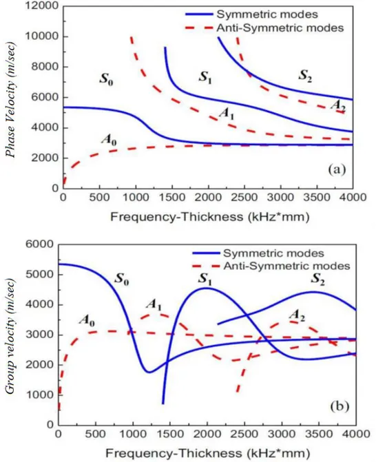
These equations can be solved numerically in an iterative way (e.g. through a bisection or a Newton-Raphson algorithm) to find different solutions, hence different dispersive modes within the same family. For sake of clarity, two plots of the dispersion relations for a 2 mm thick aluminium plate, considering both the phase (a) and the group (b) velocities, are depicted in figure 2.7 [29].

(28)

Regarding the dispersive property, it is possible to infer that, below a certain frequency-thickness product, the phase and group velocities of S0 are almost constant, hence this mode

may be considered as very low dispersive within this range.

A closer look to figure 2.7 also reveals that just one symmetric and one anti-symmetric mode exist underneath a specific threshold of the frequency-thickness product. They are named as

fundamental modes and are denoted respectively by S0 (for the symmetric mode) and A0 (for

the anti-symmetric mode). Higher order harmonics are labelled with an increasing subscript number and exists only above the aforementioned threshold.

From these graphs it is also evident that usually multiple modes are contemporary superposing and propagating through the material. A peculiarity is that they don’t interfere with each other and, therefore, the resulting motion is generated by superposition of the different modes. To excite a single mode, either the symmetric or the anti-symmetric, it is necessary to respectively input a disturbance along the longitudinal or along the out-of-plane direction of the plate; this is due to the main extensional or transversal nature of the modes. For this reason, the S0 mode is more visible along the longitudinal displacement, while A0 is more visible in the

transversal displacement.

Another positive features of the fundamental modes is that they both possess different group velocities, therefore, if the sensors’ location is far enough from the actuation point, there is enough time for the two modes to separate and be clearly visible and analysable. This characteristic is very helpful in the so-called “mode selection” process, in which specific modes are separated from the general signal in order to perform a targeted analysis. This is done since one mode may carry some particular information about the damage due to the unique interactions occurred.

These reasons show why many of the researches try to focus on the lower range of the frequency-thickness parameter: the generated modes are here easier to process, therefore it is possible to push towards more pioneering results otherwise not reachable due to the complex analysis of the chaotic and multiple wave packets contemporary moving through the material. A key aspect in using GLW for non-destructive evaluations (NDE) purposes is indeed the triggering of a particular subset of modes that propagate well and give fairly clear echoes, instead of generating the whole set of waves with the ultimate result of just complicating the overall situation.

Besides dispersion, of primarily importance is also reflection and attenuation. The latter is a phenomena, better addressed in section 4.4.3, comprising geometrical spreading, material damping and scattering.

(29)

2.3. Piezoelectricity and few general features about PZT transducers

The proper definition of piezoelectricity (whose effect was discovered in 1880 by the Curie brothers) encloses the capacity, some solid materials possess, of generating electric charge when a mechanical stresses is enforced on them. The word, derived from the Greek language, means indeed “electric charge coming from pressure”. The piezoelectric effect is reversible: this means that due to an applied electric field the material undergoes mechanical strain. However, these effects are possible only if the material possesses a net polarization along a specific direction [62].

Some materials exhibiting this behaviour are crystals (e.g. quartz), organic matter (e.g. collagen in human bones), and some ceramics (e.g. lead zirconate titanate). The ceramic materials have a significantly higher piezoelectric constant with respect to the natural crystals and they can be produced by cheap sintering processes. However, there is a drawback: their piezoelectric effect degrades in time and this loss is also related to the temperature they are exposed to.

Some new crystal materials are coming to the market, one of them is the Lead Magnesium Niobate-Lead Titanate (PMN-PT): it offers an improved sensitivity with respect to the Lead Zirconate Titanate but it possesses a lower maximum operating temperature and a higher manufacturing cost [63].

The most famous piezoelectric material exploited for the construction of acoustic transducer’s elements is the Piezoelectric Lead Zirconate Titanate (PZT). It is a ceramic compound, it appears as an insoluble white solid and it has very good piezoelectric, ferroelectric and pyroelectric properties extremely useful for the construction of electrical transducers3.

___________________________________________________________________________ 3_{The word “transducer” means that this device is capable of transforming a strain into an electrical pulse and}

vice-versa according to its function as a sensor or as an actuator.

(30)

The piezoelectric effect is exploited in several applications, from the quality assurance to the process control measurements. The one of interest for this thesis is the dynamic generation and detection of acoustic waves using small, light and cheap devices [24].

PZT transducers may be surface mounted or embedded in the airframe, thus constituting the sensing “neural network” the structure needs for developing a proper SHM system.

The PZT wafer transducer operates differently from the conventional ultrasonic probes employed nowadays for the airframe’s NDE. The differences are in the excitation mechanism of the Lamb waves, the sensor-structure coupling, the nature of the device itself and, more simply, the size and cost. Despite these differences, the PWAS proved to constitute a good alternative to the ultrasonic probes due to the favourable characteristics mentioned inside reference [30].

(31)

CHAPTER 3

3. OVERVIEW

In this chapter, an overview of the thesis’ main topics is presented. All the general choices and aspects that will be encountered throughout this study are listed and addressed, starting from the general methodology exploited in the development of the whole work until coming to the introduction of Artificial Intelligence and, in particular, of Machine Learning.

3.1. Methodology

This study has originally been thought including an experimental part in order to collect AE signals related to crack propagation however, due to the SARS-CoV-2 global pandemic, it was not possible for the author to go to Clarkson University (NY, USA). For this reason, numerical simulations have been enforced for the data collection process after having analysed two different kind of software. More specific information about the simulations are given in the next section (3.2) and especially in Chapter 4.

The main idea driving this study, as mentioned in section 1.2, is to exploit Machine Learning algorithms to identify, as final aim, the size of a small discontinuity, thus performing the so-called damage quantification. The purpose is to create a set of samples for every simulation that, theoretically, the algorithms are able to recognize, and to validate them all with the “leave

one out” cross-validation process. The choice of this validation procedure lies in the

impossibility of creating a large enough dataset just through numerical simulations, due to reasonable time limitations.

The first part of the thesis was developed on a thin pristine aluminium plate where input signals, made of Hanning windows applied to five cycle sinusoidal functions with different central frequencies1, were numerically generated at position 152.4 x 152.4 x 1.6 mm 2. The outputs were then employed in order to get confident with wave propagation simulations, verify the suitability of a numerical model in terms of wave’s characteristics but, most importantly, to understand which software should be employed to carry out the copious simulation campaign as efficiently as possible. The choice was indeed between the famous Abaqus CAETM_and

___________________________________________________________________________ 1_{Refer to section 4.1 for a detailed explanation about their usage.}

(32)

OnScaleTM; a comprehensive explanation about this topic is given in section 4.3.

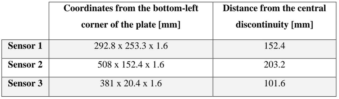
The subsequent and key part of this study was then developed on the same metal plate but with a through-thickness discontinuity placed at the centre. This time, the output signals are expected to vary according to the dimensions of the defect they are interfering with, and actually the ultimate goal of the thesis is to demonstrate that some size-related features inside the signals can be automatically recognized. Three sensors were placed at various positions on the plate in order to collect the raw signals with which to train the Machine Learning algorithms, while having also a ToA difference between them. The sensor’s position followed the non-interaction recommendation given by Hamstad et al. in [31]:

𝐷

𝑠

≥ 7

(3.1)

where D is the distance from any other similar device or from the actuator/source and s symbolizes the actuator/source’s size.

Coordinates from the bottom-left corner of the plate [mm]

Distance from the central discontinuity [mm]

Sensor 1 292.8 x 253.3 x 1.6 152.4

Sensor 2 508 x 152.4 x 1.6 203.2

Sensor 3 381 x 20.4 x 1.6 101.6

Because of the theoretically unknown defect’s position, the incident GLW usually impinge on it obliquely. Moreover, the lack of external factors contributing to the variation of experimental results compared with a numerical simulation environment, imposed the creation of a fictitious way to give a sort of randomness to the collected results. Eventually, it was decided to consider some orientations’ variation, together with the different sizes, in order to accomplish this latter task.

All these considerations led the author to choose the aforementioned sensors’ positions and four different angles as varying orientations.

___________________________________________________________________________ 2_{In section 4.4.1 the axis’ origin is displayed in a figure summing up the overall model’s geometry.}

(33)

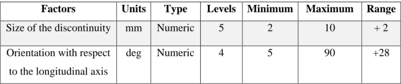
The full factorial design process for the simulation campaign was eventually made of twenty runs, resumed in the following table:

Factors Units Type Levels Minimum Maximum Range

Size of the discontinuity mm Numeric 5 2 10 + 2

Orientation with respect to the longitudinal axis

deg Numeric 4 5 90 +28

It is important that the defect is detected well below becoming visible, in the early stages of its growth. As already reported in section 1.2, the common NDE techniques have a resolution of a couple of millimetres (e.g. eddy currents) or even less, with a corresponding PoD value ranging from 70 to 80 %.

The aim of this novel automated technology is to be comparable with the existing ones, thus seeing whether also small defects are detectable with sufficient accuracy. Indeed, in most of the literature researches involving GLW interacting with damages, only large discontinuities (above 10 mm) are studied.

After the raw signals were collected, they were firstly examined and later processed. Then, many Machine Learning algorithms were trained in order to evaluate if they were able to give satisfactory predictions about the discontinuity’s size.

Resuming what has been explained above, the proposed methodology aims to simultaneously identify different damage-related signals linked to the discontinuity’s characteristics, and to exploit them to train pre-built algorithms rather than working directly on every single feature extracted from the received signal, as most of the contemporary methods do. The final purpose, together with the futures studies that will come, is indeed the development of a damage-size

classifier / predictor.

3.2. Simulation outlines: the choice of an active method

There are usually two fundamental steps to be followed in order to generate an acoustic emission through crack growth: firstly, the material’s failure accompanied by the formation of new crack surfaces, and secondly, the propagation of the resulting displacement field as a

(34)

transient wave. As an example, Lysak proposed in [32] an analytical approach involving the fracture mechanics and the wave propagation theories in order to address the acoustic waves generated by the material’s breaking. The model has some lacks in the propagation phase, where the complexity of analytically describing the wave guide problem arises. Therefore, numerical FE simulations and actual experiments are usually exploited in the majority of the studies.

Throughout the recent years, researchers have been trying to make use of various numerical methods in order to model AE sources.

To accomplish this task, numerical simulations exploit mainly two different paths: one generating a signal which is more related to the reality but difficult to be properly characterized, and the other where the source signal has some common characteristics with an hypothetical real wave but it is actually an explicitly user defined force-time curve.

In between there could be the method proposed by Lee et al. in [33] where the pre-cracked model is firstly subjected to a static load and then the nodes around the crack tip are released simulating the crack growth through an element and exciting the wave modes. However, this approach may be too simplistic because most of the major phenomena affecting a real crack growth are missing.

Simulations belonging to the aforementioned first path make often use of experimental parameters like loads, material’s constitutive equations and failure criteria based on the mechanics in order to define the proper conditions for the defect to grow. A criteria may be, for example, the degradation of the stiffness vector evaluated using as reference the geometrical position of the fracture surfaces [34]. In this paper by Markus G. R. Sause, the simulation is performed in three steps: first, a static load is applied to the structure, then the crack propagation occurs eventually followed by the signal propagation.

Simulations belonging to the second path are based on point-like AE sources where concentrated forces act. The dynamic law of these forces acting as AE source is usually found by fitting experimental data or by assumptions deriving from fracture mechanics. Various step functions describing the displacement of the crack surfaces exist, and a famous one is reported in [31] by Hamstad et al. This particular technique involving dipoles (point-like couples placed on opposite side of the crack surfaces) exploits a user-defined cosine bell function (reported in figure 3.1) and it was used to find crack length related features [17], [18], [35].

An important parameter in the definition of the source dynamic is the step functions’ rise-time because it has to represent as closely as possible the crack opening displacement time.

(35)

In [35] the authors state that there are no literature evidences of rise-time actual measurements, therefore this parameter is usually estimated by using the elastic material properties.

As mentioned before, the data collection process was supposed to be performed experimentally, therefore, to maintain the same work flow, the original aim of the thesis was to simulate a passive signal from the crack opening that could well resemble the experimental one.

In light of what stated until now throughout this section, the method to pursue this aim would have been to exploit the Crack Tip Opening Displacement 3 (CTOD) applied to the crack surface nodes. This displacement would have been theoretically able to generate a signal starting from the sudden movements of the nodes.

The issue of creating a crack growth model generating a realistic signal lies in the precise definition of the material’s failure criteria and, most importantly, of the plastic zone developed around the crack.

A very precise modelling is required if large plastic deformations are expected prior to failure and, considering the ductile material under examination (aluminium), it is clear that plasticity would greatly affect the crack growth behaviour. Crack closure’s phenomena and all the stresses induced in the nearby area are examples of this problem.

___________________________________________________________________________ 3_{Many notions regarding this parameter can be found in [64]-[65].}

(36)

A proper evaluation and representation of all these factors is crucial, since they have a direct effect on the opening load and on the CTOD which, in turn, have consequences on the generated signal. Moreover, there could be also the possibility of having a generated high frequency signal, thus exciting the higher order modes and complicating enormously the successive signal analysis.

To resume, the following features have to be properly assessed and modelled in order to have the realistic generation of an AE signal within a numerical environment:

- Plasticity must be reasonably modelled in order to have a correct crack growth and therefore a correct crack surface’s displacement leading to a consequent realistic wave propagating through the material;

- The material’s proper failure criterions must be defined in order to have a realistic growth of the defect. These derive from multiple testing campaigns performed on specimens, where the measured parameters are employed, through some mathematical models, to create and improve the numerical one [36].

- The dynamic load must be defined, based on some realistic criteria (e.g. peak, stress ratio), and the number of cycles corresponding to a specific crack length must be assessed. Moreover, when dealing with dynamic loads, it is important to distinguish between signals generated from the crack opening (labelled as “primary”) and from the crack closure (labelled as “secondary”), meaning when the two surfaces go back in contact. Both could be possibly exploited to get complementary results [37].

The impossibility of performing the experimental tests necessary to validate and refine the numerical model reduced the chances that a so-developed passive methodology could give realistic results. As an example, the method used in [38], where the local degradation of the material properties is considered as the growth driving factor, could be a viable path. However, no experimental confirmations were specified, therefore it is not clear whether the plasticity modelling through a strain-hardening function was sufficiently realistic. Moreover, it was also evident that the difference between considering or not this aspect led to non-negligible changes in the results.

Because of the aforementioned reasons and due to the primary goal of this thesis, which is not related to the correct modelling of a crack growing inside the material but rather to determine whether some crack-related signal’s patterns could be automatically recognized, it was decided to exploit an active generation technique having an input signals interfering with discontinuities

(37)

of different size directly drawn into the plate. The simulations were therefore performed exploiting the so-called pitch-catch methodology.

3.3. Techniques of signal analysis

Since the damage characterization is practically subjected to the interpretation of the recorded signals, before looking at the mathematical methods usually employed for signal analysis it is also important to state some characteristics of a time domain signal.

When an experimentally recorded signal is received, it is vital to discriminate it from the background noise and interferences (that are practically always present and varying) before analysing it. This process aims to identify the so-called hits of the signal, which are defined as transient wave packets isolated from the acquired waveform.

There are many techniques involved in detecting those hits. A detailed description of them all is outside the scope of this thesis, but the interested readers can find some of them in reference [20]. Conventionally, the most used technique consists in comparing the received signal with a specific threshold. The latter can be fixed or continuously adjusted in order to always stay just above the noise amplitude level present at that time. When the signal’s amplitude overcomes the set threshold, a single hit is detected and it lasts until there are no more threshold crossing. Since the signals collected in this thesis actually come from numerical simulations (hence from an “ideal” environment), there is no need to perform the aforementioned discrimination. Background noise will not be present, therefore the amplitude recorded before the arrival of the desired signal should be null.

(38)

Some of the key characteristics associated to each hit, highlighted in figure 3.2, are: - The peak amplitude, reached after the so-called rise time;

- The counts, which are the number of recorded peaks overcoming the threshold; - The duration, determined by the time difference between the first and the last counts; - The MARSE energy (Measured Area under the Rectified Signal Envelope), that does not have to be confused with the True energy (the area under the envelope squared).

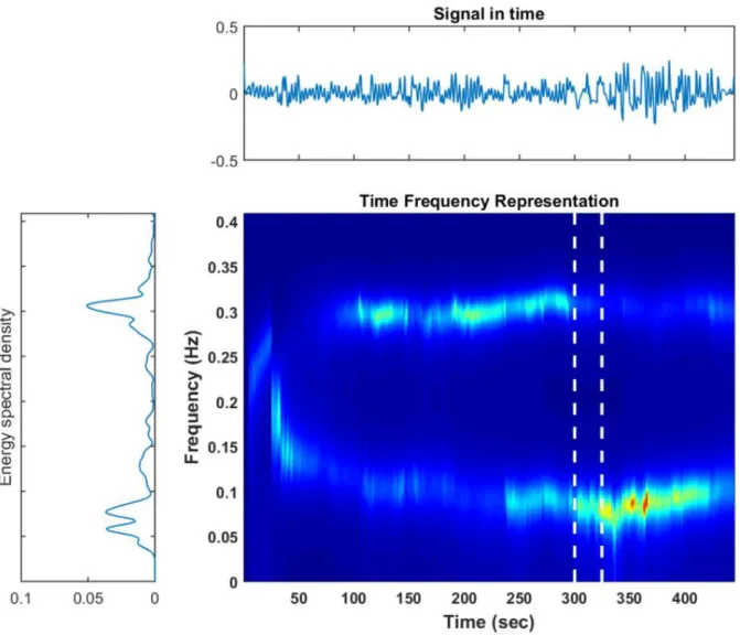
Simple time domain analysis of signals have been used to detect damages, for example by comparing the recorded signal with an undamaged benchmark (i.e. a baseline) [39]. However, the most common way to examine a signal is usually through its frequency domain (via the Fourier transform), even if this transformation leads to a complete loss of the temporal history. There are also other techniques aimed at keeping as much information as possible from both the domains: they are labelled as “time-frequency representations”.

In the following two sections, some signal processing techniques are explained.

3.3.1. Hilbert transform

Considering a time domain signal x(t), this transform allows to construct its mutual complex signal, also called analytic signal, through the following expression (3.2) [40]:

𝑥_𝐴(𝑡) = 𝑥(𝑡) + 𝑗𝐻[𝑥(𝑡)] = 𝑥(𝑡) + 𝑗 1 𝜋∫ 𝑥(𝜏) 𝑡−𝜏 𝑑𝜏 +∞ −∞ = 𝑒(𝑡) 𝑒 𝑗 𝜑(𝑡) _(3.2)

The analytic signal is made of a real part coinciding with x(t), and an imaginary part representing the signal x(t) phase-shifted by 90° (in other words, the initial signal is quadrature filtered).

The envelope e(t) and the instantaneous phase φ(t) can be derived exploiting respectively the equations (3.3) and (3.4) [40]:

𝑒(𝑡) = √𝑥(𝑡)2_{+ 𝐻[𝑥(𝑡)]}2

_(3.3)

𝜑(𝑡) = 𝑎𝑟𝑐𝑡𝑎𝑛𝐻[𝑥(𝑡)]

𝑥(𝑡) [𝑟𝑎𝑑] (3.4)

Equation (3.4) is obtained applying the definition of argument of a complex number. Moreover, the argument’s time derivative allows to calculate the instantaneous frequency:

𝑓_{𝑖𝑛𝑠𝑡} = 1

2𝜋 𝑑 𝜑(𝑡)