Search for neutral MSSM Higgs bosons with CMS at LHC: a comparison between a cut-based analysis and a Machine Learning approach

(1)

Alma Mater Studiorum · Universitá di Bologna

Scuola di Scienze

Dipartimento di Fisica e Astronomia Corso di Laurea in Fisica

Search for neutral MSSM Higgs bosons

with CMS at LHC: a comparison

between a cut-based analysis and a

Machine Learning approach

Relatore:

Prof. Daniele Bonacorsi

Correlatori:

Dott.ssa Federica Primavera

Dott. Stefano Marcellini

Dott. Tommaso Diotalevi

Presentata da:

Giordano Paoletti

(2)

(3)

(4)

(5)

Sommario

Con l’avvento della fase ad Alta Luminosità di LHC (HL-LHC [1]), la luminosità istantanea del Large Hadron Collider del CERN aumenterà di un fattore 10, oltre il valore di progettazione. La Fisica delle Alte Energie si dovrà quindi confrontare con un notevole aumento della quantità di eventi raccolti, consentendo l’indagine di scale energetiche ancora inesplorate.

In questo contesto si colloca la ricerca di bosoni di Higgs neutri aggiuntivi, previsti dalle estensioni del Modello Standard, quali ad esempio quella del Modello Super-simmetrico Minimale, teoria che suppone l’esistenza di altri bosoni di Higgs, più massivi di quello rilevato nel 2012 [2].

Alcune precedenti ricerche sono state condotte dai diversi esperimenti di LHC; in particolare per questa tesi è stata presa come riferimento l’analisi pubblicata nel 2019 dalla Collaborazione CMS [3], ricercando i bosoni di Higgs in uno stato di decadimento finale µ+_µ− _{in un range di massa tra i 130 e i 1000 GeV, prodotti}

dalla collisione di protoni ad una energia del centro di massa di 13 TeV.

Con il nuovo upgrade di LHC sarà possibile estendere il range di massa in cui ricercare i bosoni fino ad oltre 1 TeV può quindi dimostrarsi conveniente l’utilizzo di nuove tecniche e strumenti di analisi che utilizzano algoritmi di Machine Learning. In questo modo sarebbe possibile incrementare il livello di complessità dell’analisi, includendo eventualmente tra le variabili di ingresso anche l’ipotesi di massa in-iziale del bosone di Higgs supersimmetrico ed ottenendo un modello sempre più generalizzato.

In questa tesi vengono confrontati i risultati della classificazione tra eventi di segnale ed eventi di fondo di un’analisi "tradizionale" cut-based, sulla base di quella di riferimento, e un’ analisi multivariata condotta utilizzando una BDT implementata in ROOT.

I risultati confermano un possibile miglioramento nella classificazione tra segnale e fondo, utilizzando un’analisi multivariata.

Il Capitolo 1 fornisce una panoramica di LHC, con maggiore attenzione all’esperimento CMS.

Il Capitolo 2 presenta una panoramica dei modelli in Fisica alle Alte Energie, in particolare il Modello Supersimmetrico oltre il Modello Standard.

Nel Capitolo 3 vengono presentati gli strumenti utilizzati in questa tesi per realizzare le due analisi proposte, quali ROOT e TMVA.

Il Capitolo 4 spiega e compara l’ analisi cut-based e multivariata, riportando i risultati conclusivi.

(8)

(9)

Abstract

With the advent of the High Luminosity phase of LHC (HL-LHC [1]), the instantaneous luminosity of CERN’s Large Hadron Collider will increase by a factor of 10, beyond the design value. The High Energy Physics, therefore, will have to bare with a considerable increase in the amount of collected events, enabling the investigation of still unexplored energy scales.

In this context, the search for the neutral Higgs bosons theorized by the Super-symmetric Model beyond the Standard Model finds its place; this theory in fact supposes the existence of other Higgs bosons, more massive than the one discovered in 2012 [2].

Some previous researches has been conducted by LHC experiments; in particular this thesis take as a reference the analysis published in 2019 by the CMS Collabo-ration [3], which looks for the Higgs bosons in a final state µ+_µ− _{and in a mass}

range between 130 and 1000 GeV, produced by the collision of protons at a center of mass energy of 13 TeV.

With the new LHC upgrade, the search range of such bosons may be extended to over 1 TeV; therefore the usage of new techniques and analysis tools based on Machine Learning can prove to be helpful. In this way, it is in fact possible to increase the level of complexity of the analysis, even by adding in the future the initial mass hypothesis of the Higgs bosons as an input variable, obtaining a model as general as possible.

In this thesis, the results of the classification between signal and background events with both a ¨traditional¨cut-based approach, using the reference published paper, and a multivariate analysis conducted using a Boosting Decision Trees implemented in ROOT are compared.

The results show a possible improvement in the signal versus background classifica-tion, by using a multivariate analysis.

Chapter 1 provides an overview of LHC, with more attention to the CMS experi-ment.

Chapter 2 presents an overview of the High Energy Physics models, in particular the Supersymmetric Model beyond the Standard Model.

Chapter 3 briefly describes the tools used in this thesis to carry out the two proposed analyses, i.e. ROOT and TMVA.

Chapter 4 explains and compares the cut-based and multivariate analysis, report-ing the conclusive results.

(10)

(11)

Chapter 1 High Energy Physics at the LHC

1.1 General introduction to LHC

The Large Hadron Collider (LHC) [4,5] is part of the CERN accelerator complex (see Figure 1.1) [6], in Geneva, and it is the most powerful particle accelerator ever

built.

LHC is located in the 26.7 km long tunnel that was previously hosting the LEP (Large Electron-Positron) collider [7], about 100 m under the French-Swiss border close to Geneva. LHC accelerates and collides proton beams at an unprecedented center of mass energy up to √s= 13 TeV in order to be able to test the Standard Model (SM) predictions to a high level of precision, as well as to search for physics Beyond SM [8].

The LHC basically consists of a circular circumference ring, divided into eight

Figure 1.1: The accelerators chain at CERN.

independent sectors, designed to accelerate protons and heavy ions. These particles travel on two separated beams on opposite directions and in extreme vacuum

(12)

CHAPTER 1. High Energy Physics at the LHC

conditions [9]. Beams are controlled by superconductive electromagnets [10], keeping them in their trajectory and bringing them to regime.

Some of the main LHC parameters are shown in Table 1.1.

The various data collection periods are characterized by a quantity called Luminosity L: it is defined as

L = f n1n2 4πσxσy

(1.1) where ni is the number of particles in the bunch, f is the crossing frequency and σx, σyare the tranverse dimensions of the beam.

As already mentioned above, it characterizes the data collection periods and it is necessary to take this into account for a correct comparison with the expectation in the analysis phase;in fact knowing the production cross section σp of a physical process, we can then calculate the event rate R(that is, the number of events per second) as:

R= Lσp (1.2)

The number of protons per bunch is N∼ 1011 _{so this implies the probability of}

overlapping events in the same time of data acquisition, referred to as pile-up (PU).

Table 1.1: Main technical parameters of LHC.

Quantity value

Circumference (m) 26 659

Magnets working temperature (K) 1.9

Number of magnets 9593

Number of principal dipoles 1232

Number of principal quadrupoles 392

Number of radio-frequency cavities per beam 16

Nominal energy, protons (TeV) 6.5

Nominal energy, ions (TeV/nucleon) 2.76

Magnetic field maximum intensity (T) 8.33

Project luminosity (cm−2_s−1₎ _{10 × 10}34

Number of proton packages per beam 2808

Number of proton per package (outgoing) 1.1 × 1011

Minimum distance between packages (m) ∼7

Number of rotations per second 11 245

Number of collisions per crossing (nominal) ∼20

Number of collisions per second (millions) 600

The four main experiments that collect and analize data from the particle collisions provided by the LHC are:

• A Large Ion Collider Experiment(ALICE) (see Section A.1): an experiment that mainly uses Pb-Pb dedicated collisions focusing to study quark-gluon-plasma;

(13)

1.2. AN OVERVIEW OF THE CMS EXPERIMENT

• A Toroidal LHC ApparatuS(ATLAS) (see SectionA.2) and

Compact Muon Solenoid(CMS) (see Section1.2): two general purpose exper-iments;

• LHC beauty experiment(LHCb) (see Section A.4): an experiment specialized in the study of quark-antiquark asymmetry.

1.2 An overview of the CMS experiment

The CMS main purpose is to explore the p-p physics at the TeV scale. Its cylindrical concept is built on several layers and each one of them is dedicated to the detection of a specific type of particle; in particular, the CMS experiment has its prominent feature in revealing muons with good resolution.

About 4300 people including physicists, engineers, technicians and students work actively on CMS experiment.

1.2.1 The CMS detector: concept and structure

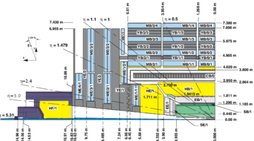
As mentioned above, the CMS detector is made up of different layers, as illustrated in Figure1.2. Each of them is designed to trace and measure the physical properties and paths of different kinds of subatomic particles. Furthermore, this structure is surrounded by a huge solenoid based on superconductive technologies, operating at 4.4 K and generating a 4 T magnetic field.

The first and inner layer of the CMS detector is called Tracker [11, pp. 26-89]: made entirely of silicon, is able to reconstruct the paths of high-energy muons, electrons and hadrons as well as observe tracks coming from the decay of very short-lived particles with a resolution of 10 nm.

The second layer consists of two calorimeters, the Electromagnetic Calorimeter (ECAL) [11, pp. 90-121] and the Hadron Calorimeter (HCAL) [11, pp. 122-155] arranged serially. The former measures the energy deposited by photons and electrons, while the latter measures the energy deposited by hadrons.

Unlike the Tracker, which does not interfere with passing particles, the calorimeters are designed to decelerate and stop them.

In the end, there are a superconductive coil and the muon detectors alternated with iron layers (to uniform the magnetic field lines as much as possible) [11, pp. 162-246] able to track muon particles, escaped from calorimeters. The lack of energy and momentum from collisions is assigned to the electrically neutral and weakly-interacting neutrinos.

1.2.2 Trigger and Data Acquisition

When CMS is at regime, there are about a billion interactions p-p each second inside the detector. The time-lapse from one collision to the next one is just 25 ns so data are stored in pipelines able to withhold and process information coming from simultaneous interactions. To avoid confusion, the detector is designed with an excellent temporal resolution and a great signal synchronization from different channels (about 1 million).

(14)

CHAPTER 1. High Energy Physics at the LHC

(a) Section view. (b) View along the plane perpendicular to beam

direction.

Figure 1.2: Compact Muon Solenoid.

Given the large number of events resulting from the collision between protons, it is necessary that the experiment has a trigger system to pre-select the most interesting events to record [11, pp. 247-282]; it is organized in two levels: the first one is hardware-based, completely automated and extremely rapid in data selection. It selects physical interesting data, e.g. an high value of energy or an unusual combination of interacting particles. This trigger acts asynchronously in the signal reception phase and reduces acquired data up to a few hundreds of events per second. Subsequently, they are stored in special servers for later analysis. Next layer is software-based, acting after the reconstruction of events and analyzing them in a related farm, where data are processed and come out with a frequency of about 100 Hz.

1.2.3 CMS Coordinate system

The CMS coordinate system used to describe the detector is a right-handed Cartesian frame, centred in the interaction point and with z axis along the beam line(this direction is referred to as longitudinal) from the LHC point 5 to the mount Jura. The x axis is chosen to be horizontal and pointing towards the centre of the LHC ring, and the y axis is vertical and pointing upwards. The x-y plane is called transverse plane.

Given the cylindrical symmetry of the CMS design, usually a (ϕ,θ) cylindrical coordinate system is used in the reconstruction of the tracks of particles. The polar angle is ϕ(∈ [0, 2π]), laying in the x-y plane, measured from the x-axis in mathematical positive direction (i.e. the y-axis is at ϕ=π₂). The azimuthal angle θ(∈ [−π

2, π

2]) is measured from the z-axis towards the x-y plane. The angle θ can be translated into the pseudo-rapidity η by

η = −ln(tanθ

2) (1.3)

The actual value of η can be seen in the longitudinal view of the detector in 1.3. Using these parameters, the distance between two particles can be defined as

∆R =q∆ϕ2+ ∆η2 (1.4)

(15)

1.2. AN OVERVIEW OF THE CMS EXPERIMENT

Figure 1.3: Longitudinal view of the CMS subdetectors, with the indication of the

pseu-dorapidity η value at different angles θ.

Referring to the Cartesian system, the momentum of a particle can be divided in two components: the longitudinal momentum pz and the transverse momentum pT, defined as:

pT =

q

p2

x+ p2y (1.5)

The magnet bends charged tracks on the ϕ plane, so what is effectively measured is the pT of the particles.

1.2.4 Events reconstruction in CMS

The particle flow (PF) algorithm, that combines the information from all the sub-detectors, is used to reconstruct the full event. It combines the information from all subdetectors to reconstruct individual particles identifying them as charged or neutral hadrons, photons or leptons and to determine the missing energy transverse. Electrons and muons are formed by associating a track in the silicon detectors with a cluster of energy in the electromagnetic calorimeter, or a track in the muon system. Jets are reconstructed using tracks and calorimeter informations.

The quantity Missing Energy transverse (Emiss

T ) is defined as the magnitude of the negative vector sum of the transverse moment of all the PF objects (charged and neutral) in the event. It is used to infer the presence of non-detectable particles such as neutrinos and is expected to be a signature of many new physics events. In hadron colliders, the initial momentum of the colliding partons along the beam axis is not known, however the initial energy in particles travelling transverse to the beam axis is zero, so any net momentum in the transverse direction indicates Missing Transverse Energy.

An algorithm that reconstructs secondary vertices is used to identify jets resulting from the hadronization of b quarks. The algorithm can be applied to jets with pT>20GeV in the pseudorapidity range η < 2.4. For jets emitted within this kinematic range, the efficiency of the algorithm is 66% with a missing tag probability of 1% for the selected working point.

(16)

(17)

Chapter 2 Physics of the MSSM neutral

Higgs bosons

This chapter gives a short presentation of the physical theories at the basis of the search for MSSM Neutral Higgs bosons in the µ+_µ− _{final state at s=}√_{13 TeV;}

in particular:

• In section 2.1 there is a summary of the main aspects of the Standard Model and it is briefly stated the reason why it is not complete;

• In section2.2 the main features of the most common theories beyond SM are given

• In section 2.3 there is an overview of the Supersymmetry (SUSY) theory and the MSSM Higgs bosons production.

• In section 2.4.2 the most relevant background events are shown.

2.1 The Standard Model SM: an incomplete model

2.1.1 Introduction to SM

The Standard Model represent, currently, the best description owned of the elementary particles and of their interaction. It models two Gauge theories: the electroweak interaction, which unites the electromagnetic and weak interactions, and the strong interaction, also called Quantum Chromodynamics (QCD). The fundamental structures of matter, quarks and leptons, are described by fermions with half spin, while interactions are mediated by bosons, with integer spin. The symmetry group of SM is:

SUC(3) × SUL(2) × UY(1),

where the first factor describes the strong interaction of color, mediated by 8 gluons, while SUL(2) × UY(1) is the group which describes the electroweak unification, mediated by photon and bosons Z0 and W±.

Gauge theories do not contain the mass terms of the bosons, in fact it would cause a renormalization problem, but experimentally the opposite has been observed; the

(18)

CHAPTER 2. Physics of the MSSM neutral Higgs bosons

solution is the introduction of a scalar particle, Higgs boson, capable of mating with other particles giving them mass through the spontaneous symmetry breaking mechanism. Higgs mechanism allows to give a mass to each fermion except for neutrinos, fotons and gluons.

SM has been studied extensively in the last decades, especially thanks to the contributions given by LEP and Tevatron; its great success is due to the abil-ity to accurately describe the phenomenology of elementary particles observed experimentally, demonstrating an extraordinary agreement between theory and experiment.

2.1.2 The reason to go beyond SM

Despite the completeness and the successes of the SM, there are some unresolved problems, both from a theoretical and an experimental point of view.

The gaps suggested by the observation are substantially four:

• the neutrinos mass is not provided by SM, while it is known (thanks to neutrino flavour oscillation) that they have a non-zero mass, lower than the electronvolt;

• there is no candidate for the Dark Matter (DM), which represent almost 80% of the universe matter;

• Inflation dynamics is not predicted;

• Asymmetry matter-antimatter is not justified.

Instead from the theoretic point of view there are the following open questions:

Flavour problem and high number of free parameters The SM needs of 18

free parameters: 9 fermions masses; 3 angles for Cabibbo-Kobayashy-Maskawa (CKM) matrix and 1 complex phase; the strong, the weak and the

electro-magnetic coupling parameter (αS, αW, αEM); Z0 and Higgs bosons mass.

Therefore SM is not a very predictive model, in fact it doesn’t expect any mass, and neither it estimates their mixing, moreover it doesn’t give any bond on the number of fermions family. Then there are other parameters not included in the model, coming from neutrino oscillation’s physics: 3 angles of mixing and the complex phase of Pontecorvo-Maki-Nakagawa-Sakata matrix.

Gauge hierarchy problem From Quantum Field Theory it is known that the

perturbative corrections tend to increase the mass of scalars, bringing it to a value close to the energy scale in which the theory is considered valid [12]. Admitting that SM is a low energy approximation of a wider theory also valid for high energy i.e. Planck scale (∼ 1019_{GeV), there is the need that it is able}

to maintain Higgs bosons mass in the order of 100 GeV; however within the SM the radiative corrections to the mass of the Higgs due to hypothetical mass particles equal to MP lanck diverge the mass of the Higgs.

(19)

2.2. BEYOND STANDARD MODEL THEORIES (BSM)

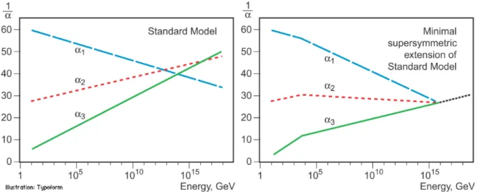
Unification problem Even without considering gravitational interaction, a real

unification theory of three other interactions does not exist: each one has their own gauge group and their own running coupling constant α which behaves differently depending on the energy range: as it can be seen in Fig.2.1 SM does not provide the correspondence between constants.

Figure 2.1: Dependence of α on Energy in the SM and in the MSSM (introduced in sec.

2.2).

Mass scale problem An unresolved problem is why in the Standard Model masses

of fermionic particles range from the eV order for neutrinos (perhaps very overestimated limit) to the hundred GeV of the quark top.

2.2 Beyond Standard Model theories (BSM)

The need to extend the Standard Model has given rise to a lot of theories that should overcome the limitations. Below there are some of the main features of the most accredited models:

• Grand Unified Theories (GUT)

These models of great unification aim to look for a group of symmetry that may include three of the four fundamental interactions: some of the possible candidates are the groups SO(10), SU(5) and E(6). It is expected that at the GUT scale, in the order of 1016_{GeV, non-gravitational interactions are}

governed by a single coupling constant αGU T (see at fig. 2.1).

While enjoying some strengths, such as the possibility of giving mass to neutrinos, these theories foresee in some cases phenomena not yet observed (decay of the proton, existence of magnetic monopolies) and are valid at

experimentally non-reproducible energies.

Some hope of finding new physics at lower scales could arise from the union between GUT and supersymmetric models.

• Supersymmetry(SUSY)

(20)

Model has a superpartner bosonic (fermionic) with the same identical quantum numbers except, obviously, the spin. The presence of s-fermions and s-bosons allows to elegantly solve the problem of the hierarchy for the Higgs mass described in Section 2.1.2, since the contributions brought by the new SUSY particles exactly cancel the divergences due to the perturbation corrections induced by the SM particles: this is possible as long as it is admitted that the coupling of Yukawa with the Higgs is identical for fermions and bosons and that the SUSY particles have mass around the TeV.

In section2.3 SUSY has been discussed more specifically. • Super-string Theory

In this group of theories, inspired by the unification of electromagnetism with gravity by Kaluza and Klein, we hypothesize the existence of dimensions beyond the four ordinary that would allow to include the gravitational interac-tion to explain its weakness compared to the other three: the accessible world would only be a brane of much larger (bulk) volume that escapes observation. The Randall-Sundrum model, in particular, postulates the existence of a fifth compact dimension: two 4-dimensional branes, the TeV-brane and the Planck-brane, are immersed in a 5-dimensional bulk. The SM particles are confined to

the TeV-brane, where the intensity of gravity is suppressed exponentially by the metric. Gravity resides in the Plank-brane, as well as the gravitons, so a Kaluza-Klein tower of excited states is admitted, which can propagate in the bulk. The possible presence of extra-dimensions would occur experimentally with the disappearance of large amounts of energy, or with more difficulty, with the emergence in the TeV-brane of particles coming from the bulk.

2.3 Supersymmetry and MSSM

Supersymmetry is a generalization of the space-time symmetries of quantum field theory that transforms fermions into bosons and vice versa. It gives to each particle its super-partner which differ in spin by half a unit.

Supersymmetry provides a framework for the unification of particle physics and gravity which is governed by the Planck energy scale MP lanck(∼ 1019 GeV), where

the gravitational interactions become comparable in strength to the gauge interac-tions. It can provide a solution to the hierarchy problem, and explain the smallness of the electroweak scale compared with the Planck scale. This is one of the problems of the SM where is not possible to maintain the stability of the Gauge hierarchy in the presence of radiative quantum corrections.

If SUSY were an exact symmetry of nature, then particles and their superpartners would be degenerate in mass. Since superpartners have not (yet) been observed, SUSY must be a broken symmetry. Nevertheless, the stability of the Gauge hierar-chy can still be maintained if the breaking is soft; that means the supersymmetry-breaking masses cannot be larger than a few TeV. The most interesting theories of this type are theories of low-energy (or weak-scale) supersymmetry, where the effec-tive scale of SUSY breaking is tied to the scale of electroweak symmetry breaking. SUSY also allows the grand unification of the electromagnetic, weak and strong

(21)

2.3. SUPERSYMMETRY AND MSSM

gauge interactions in a consistent way, as it is strongly supported by the prediction of the electroweak mixing angle at low energy scales, with an accuracy at the percent level.

An example of a theory associate to supersymmetry is the Minimal Supersymmetric extension of the Standard Model(MSSM) which associates a supersymmetric partner to each Gauge boson and chiral fermion of the SM, and provides a realistic model of physics at the weak scale.

2.3.1 Higgs production in MSSM

In the MSSM, there are five physical states of the Higgs: the neutral scalar CP-odd A0_{, the two scalar charged H}± _{and the two neutral scalars CP-even h}0 _and

H0.

Their mass is determined at the tree level from mA0 and tan(β), where tan(β) is a

fundamental parameter of MSSM that is not studied in this thesis, whose definition is reported below for completeness purposes[13]:

tan(β) is defined as the ratio between the vacuum expectations value of Higgs doublets:

tan(β) ≡ νu νd

. (2.1)

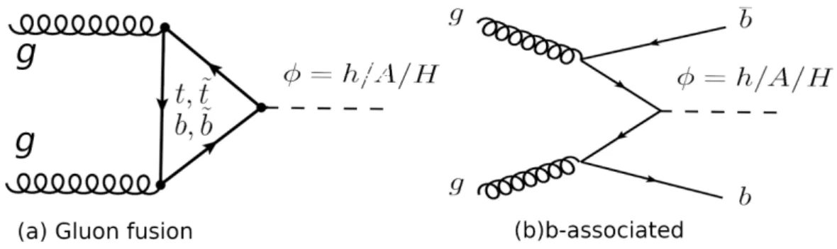
With φ we refer to the neutral Higgs bosons (A0_{, h}0_{, H}0). The production of

a neutral MSSM Higgs pp→ φ + X at LHC is dominated by two processes: the b-associated where φ is produced together with a pair b¯b, and the gluons fusion (ggφ) (see Fig. 2.2).

The coupling between the Higgs and quarks depends strongly on tan(β); in

Figure 2.2: Feynman diagrams represented the production of an MSSM Higgs boson at

the LHC in the gluon fusion process ggφ (a), and in the b-associated channel bbφ (b).

particular the coupling of φ with the quarks b increases to large values of tan(β) compared to the case of Higgs in SM:

gM SSM_b¯_bφ = tan(β) · gSM_b¯_bφ (2.2) Consequently, while for low values of tan(β)(< 15) the main production is the gluon fusion mechanism, for high values of tan(β) the b-associated production becomes dominant[13].

(22)

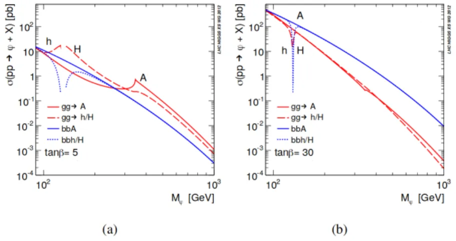
Figure 2.3: The production cross section of the φ boson as function of its mass for

tan(β)= 5(left) and tan(β)= 30(right).

The production cross section of the φ boson is shown in figures 2.3. The plots on the right (for tan(β)= 30), point out that the Higgs bosons production in association with b quarks is enhanced with respect to the plots on the left (for tan(β)= 5), by a factor 2 tan2_(β).

For the same reason the neutral Higgs decaying to b quarks has the highest branch-ing fraction, about 90% (see Fig 2.4); indeed it is the heaviest down-type fermion.

Figure 2.4: The decay branching ratios of the h boson as a function of A boson mass

Moreover, the Higgs coupling is proportional to the square of particle mass, that explains why the second favourite decay channel is the τ+_τ− _{with about 10% of}

branching fraction.

(23)

2.4. MSSM NEUTRAL BOSONS HIGGS DECAYING TO µ+µ−

2.4 MSSM Neutral Bosons Higgs decaying to µ

+

_µ

−

2.4.1 Signal events

A further MSSM Higgs decay has to be taken into account: the µ+_µ− _channel.

Despite their low branching ratio, the leptonic decays provide higher sensitivity than the b¯b decay, strongly contaminated by the large QCD background characteristic of the LHC environment. Among them, while the τ+_τ− _{process has a branching}

ratio larger by a factor (mτ mµ

)2 and provides better sensitivity in terms of statistics,

the µ+_µ− _{process has a cleaner experimental signature and benefits of the full}

reconstruction of the final state. Furthermore, thanks to precision of the muon momentum measurement at CMS, the Higgs mass can be reconstructed from µ+_µ−

decays with a better resolution, and a measurement of the tan(β) parameter can be performed.

2.4.2 Background events

In this paragraph we will briefly discuss the types of events that, producing the same final µ+_µ− _{status, complicate the search for the chosen event. In particular,}

in this thesis, two types of background events have been taken into consideration: Drell-Yan and t¯t.

Drell-Yan background

Figure 2.5: Feynman diagram of the Drell-Yan process with final state µ+µ−.

The Drell-Yan process, schematized in Fig. 2.5, represents the main background for our signal. It includes the decay of a Z/γ∗ in a pair of leptons (muons), or the creation of pairs l+_l−_(µ+_µ−_{) through QED processes. As shown in Fig.} _2.5_{, the}

pair production is identical to that of the signal.

Although the nature of the signal processes and of Drell-Yan is the same, the two phenomena have a different invariant mass spectrum: that of the signal is characterized by a peak in mass invariant in correspondence with the nominal

(24)

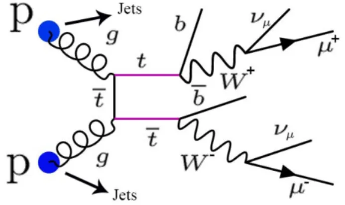
Figure 2.6: Feynman diagram of the couple decay process t¯t with final state µ+µ−.

value of mφ, while the Drell-Yan presents a continuous distribution, given from the contribution of photons to the final state.

t¯t background

Another relevant background source is the production of t¯t pairs (described in Fig. 2.6). It is a different process from the electroweak one of Z/γ and φ: in the final state over (µ+_µ−_{) jets originating from the decay of bottom quarks (b-jets) are}

also expected. This background is distributed over a large invariant mass spectrum, without giving rise to any peak.

(25)

Chapter 3 Tools for High Energy Physics

In this chapter the technical features of the tools (ROOT and TMVA) used in this thesis are described.

3.1 ROOT framework for High Energy Physics

Figure 3.1: ROOT’s logo.

ROOT is an object-oriented framework aimed at solving the data analysis challenges of High Energy Physics (HEP) [14]. It was born to replace the old interactive data analysis systems PAW [15] and PIAF [16] and the simulation package GEANT [17], written in FORTRAN, which do not scale up to future challenges of the LHC, where the amount of data to be simulated and analyzed is a few orders of magnitude larger than before.

Being a framework means that common code with generic functionality can be selectively specialized or overridden by developers or users, allowing the user to enjoy different benefits: first, less code to write because the programmer should be able to use and reuse the majority of the existing one (such as fitting and histogramming are implemented and ready to use and customize); then the code is more reliable and robust because it is made up of pieces of framework’s code already tested and integrated with the rest of the framework; users do not have to be experts at writing user interfaces, graphics or networking to use the frameworks that provide those services, etc. .

The term "object-oriented" classifies the framework as implemented in the OOP (Object Oriented Programming) paradigm.

The OOP is a high-level programming language where a program is divided into small chunks called objects. This paradigm is based on objects (basically a self-contained entity that accumulates both data and procedures to manipulate the data) and classes (a blueprint of an object which defines all the common properties

(26)

CHAPTER 3. Tools for High Energy Physics

of one or more objects that are associated with it). In short words, in ROOT data are managed by object, and methods are the only way to assess the data.

Trees: data collection objects

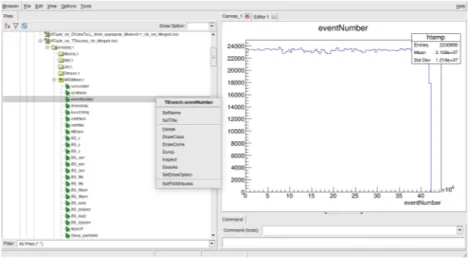
In case users want to store large quantities of same-class objects, ROOT has designed the TTree and TNtuple classes specifically for that purpose. The TTree class is optimized to reduce disk space and enhance access speed. A TNtuple is a TTree that is limited to only hold floating-point numbers; a TTree on the other hand can hold all kind of data, such as objects or arrays; in addition to all the simple types: the idea is that the same data model, same language, same style of queries can be used for all data sets in one experiment.

When using a TTree, we fill its branch buffers (class TBranch) with leaf data

Figure 3.2: Example of a root file structure.

(class TLeaf) and the buffers are written to disk when it is full. Each branch will go to a different buffer (TBasket). Some buffers will be written maybe after every event, whereas other buffers may be written only after a few hundred events. The different buffers can also be organized to be written on the same file or different files. This mechanism is also well suited for parallel architectures. Note that this scheme allows also the insertion of a new branch at any time in an existing file or set of files. Due to this data clustering scheme, queries can be executed very efficiently. Queries executed on one or more variables or objects, cause only the branch buffers containing these variables to be read into memory.

Physics vector class: TLorentzVector

TLorentzVector is a general four-vector class, which can be used either for the description of position and time (x, y, z, t) or momentum and energy (px, py, pz, E). There are two sets of access functions to the components of a TLorentzVector: X(), Y(), Z(), T() and Px(), Py(), Pz() and E(). The first set is more relevant to use when TLorentzVector describes a combination of position and time and the second set is more relevant when TLorentzVector describes momentum and energy. In this thesis the spherical coordinates was used, given the cylindrical symmetry of

(27)

3.2. TOOLKIT FOR MULTIVARIATE ANALYSIS (TMVA)

the CMS detector (See sec. 1.2.3), so a further method was used for convenience: SetPtEtaPhiM(pT, η, φ, m).

3.2 Toolkit for Multivariate Analysis (TMVA)

Figure 3.3: TMVA’s logo.

TMVA is a ROOT-integrated environment to structure a Multivariate Analysis provides tools for the processing, parallel evaluation and application of multivariate classification (and in latest release, also for multivariate regression techniques). TMVA is developed for the needs of HEP applications, but may be not limited to these.

TMVA implements multivariate techniques belonging to the so-called supervised learning algorithms, which make use of training events, with known output, to determine the mapping function that either describes a decision boundary (classifi-cation) or an approximation of the underlying functional behaviour defining the target value (regression).

The software package consists of abstract, object-oriented implementations in C++/ROOT for every multivariate analysis (MVA) technique, as well as auxiliary tools such as parameter fitting. It provides training, testing and performance evaluation algorithms and visualisation scripts.

The training and testing are performed with the use of user-supplied data sets in form of ROOT trees (See sec. 3.1) or text files, where each event can have an individual weight.

To compare the signal-efficiency and background-rejection performance of the clas-sifiers, the analysis job prints tabulated results for some benchmark values. The performance evaluation in terms of signal efficiency, background rejection, etc., of the trained and tested MVA methods is invoked by the command:

factory->EvaluateAllMethods();

The optimal method to be used for a specific analysis strongly depends on the problem at hand and no general recommendations can be given. Moreover, a variety of graphical evaluation information acquired during the training, testing and evaluation phases is stored in a ROOT output file.

Afterwards, a detailed description of the TMVA methods Boosted Decision Tree used for the scope of this thesis, and some of its options is given.

3.2.1 Boosted Decision Trees in TMVA

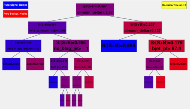
A decision tree is a classifier with a tree-structure, as shown in Fig. 3.4: starting from the root node, a sequence of binary splits using the discriminating variables,

(28)

that at this node gives the best separation between the signal and background, is applied to the data.

The phase space is split this way into many regions that are eventually classified

S/(S+B)=0.873 S/(S+B)=0.406 S/(S+B)=0.828 delta_R_bjet_dimuon< 2.42 S/(S+B)=0.891 S/(S+B)=0.674 S/(S+B)=0.385 S/(S+B)=0.503 dimuon_deltar< 3.14 S/(S+B)=0.615 bjet_pt< 51.8 S/(S+B)=0.524 S/(S+B)=0.436 S/(S+B)=0.478 bjet_eta>0.117 S/(S+B)=0.264 S/(S+B)=0.349 dimuon_deltar< 3.09 S/(S+B)=0.498 no_btag_jet> 1 S/(S+B)=0.660 delta_pt_mupair_1bjet<0.556 S/(S+B)=0.998 S/(S+B)=0.680 S/(S+B)=0.109 S/(S+B)=0.455 dimuon_deltar< 1.82 S/(S+B)=0.091 S/(S+B)=0.179 bjet_pt< 87.4 S/(S+B)=0.257 dimuon_deltar>0.127 S/(S+B)=0.497 dimuon_deltar< 2.67

Decision Tree no.: 0 Pure Signal Nodes

Pure Backgr. Nodes

Figure 3.4: Schematic view of a three-levels decision tree. The leaf nodes at the bottom

end of the tree are blue colored for the signal S and red colored for the

background B depending on the ratio S

S + B (1 is the perfect S-leaf and 0 the

perfect B-leaf).

as signal or background, depending on the majority of training events that end up in the final leaf node.

To improve the classification performance of this method (and increase the stability with respect to statistical fluctuations in the training sample) a boosting procedure is implemented; in fact, for example, if two input variables exhibit a similar separation power, a fluctuation in the training sample may cause the tree growing algorithm to decide to split on one variable, while the other variable could have been selected without that fluctuation. In such a case the whole tree structure is altered below this node, possibly resulting also in a substantially different classifier response. The boosting of a decision tree consists of extending this binary structure from one tree to several trees which form a forest. The trees are derived from the same training ensemble by reweighting events, and are finally combined into a single classifier who is given by an (weighted) average of the individual decision trees; however, the advantage of the straightforward interpretation of the decision tree is lost.

In many cases, the boosting performs best if applied to trees that, taken individually, have not much classification power. These so called weak classifiers are small trees, limited in growth to a typical tree depth of as small as three, depending on the how much interaction there is between the different input variables. By limiting the tree depth during the tree building process (training), the tendency of overtraining for

(29)

simple decision trees which are typically grown to a large depth and then pruned, is almost completely eliminated.

In this thesis the focus is on Discrete Adaptive Boost (AdaBoost, see below) method, omitting the discussion of the other possible boosting methods [18] (never used in this comparison).

In TMVA the Boosted Decision Trees (BDT) classifier is booked via the command: factory->BookMethod( Types::kBDT, "BDT", "<options>" );

where the user can customize his BDT having available several configuration.

Discrete Adaptive Boost (AdaBoost)

Adaptive Boost (AdaBoost) is the most popular boosting algorithm; in a classification problem it consists in the assignment of a greater weight, during the training of a tree, to the events which were misclassified during the training of a previous tree.

The first tree is trained using the original event weight, while the subsequent tree is trained using a modified event sample, where there is a factor α called boost weight, that multiply the weight of previously misclassified events.

The α factor is defined as

α= 1 − err

err (3.1)

where err is the misclassification rate, that, by construction, is less or equal to 0.5 as the same training events used to classify the output nodes of the previous tree are used for the calculation of the error rate.

However there is a normalization of the entire event sample, so that the sum of the sample weights remains constant.

Defining the result of an individual classifier as h(x), where x is the tuple of input variables, h(x) = ±1 for signal and background, the boosted event classification yBoost(x) is given by yBoost(x) = 1 Ncollection Ncollection X i=1 ln(αi) · hi(x) (3.2) where the sum is over all classifiers in the collection. Small (large) values for yBoost(x) indicate a background-like (signal-like) event. Equation 3.2represents the standard boosting algorithm: as shown from the schematic representation in Fig.

3.5, initially a simple classifier has been fitted on the data, also called a decision stump, which split the data into just two region, and whatever the event is correctly classified, will be given less weight edge in the next iteration; therefore, in the second iteration, misclassified events have higher weight. The second classifier is fitted, and the same procedure is repeated for the third classifier. Once it finishes the iteration, these are combined with weights that are automatically calculated for each classifier at each iteration based on the error rate, to come up with a strong classifier which predict the classes with surprising accuracy.

As previously written this boosting procedure performs bests on weak classifier, so the performance is often further enhanced by forcing a slow learning and allowing a

(30)

larger number of boost steps instead. The learning rate ("Learning rate is a hyper-parameter that controls how much we are adjusting the weights of our alghoritm with respect the loss gradient."[19]) of the AdaBoost algorithm is controled by a parameter β giving as an exponent to the boost weight α → αβ.

Figure 3.5: How AdaBoost works.

Training a decision tree

The training, building or growing of a decision tree is the process that defines the splitting criteria for each node (see fig. 3.4). The training starts with the root node, where an initial splitting criterion for the full training sample is determined. The split results in two subsets of training events that each go through the same algorithm of determining the next splitting iteration. This procedure is repeated until the whole tree is built. At each node, the split is determined by finding the variable and corresponding cut value that provides the best separation between signal and background. The node splitting stops once it has reached the minimum number of events which is specified in the BDT configuration (option nEventsMin). Among all the separation criteria, the statistical significance, defined by √ S

S+ B, was chosen. A common feature among all criteria is that they are symmetric with respect to the event classes, because a cut that selects predominantly background is as valuable as one that selects signal. Since the splitting criterion is always a cut on a single variable, the training procedure selects the variable and cut value that optimises the increase in the separation index between the parent node and the sum of the indices of the two daughter nodes, weighted by their relative fraction of events.

User can set the granularity of the scanning over the variable range, searching a satisfactory compromise between computing time and step size. In TMVA a truly optimal cut, given the training sample, is determined by setting the option nCuts=-1: this invokes an algorithm that tests all possible cuts on the training sample and finds the best one. The latter is of course slightly slower than the coarse grid.

In principle, the splitting could continue until each leaf node contains only signal 20

(31)

or only background events, which could suggest that perfect discrimination is achievable; however, such a decision tree would be strongly overtrained. To avoid overtraining a decision tree must be pruned.

Pruning a decision tree

Pruning is the process of cutting back a tree from the bottom up after it has been built to its maximum size. Its purpose is to remove statistically insignificant nodes and thus reduce the overtraining of the tree.

For Boosted Decision trees however, as the boosting algorithms perform best on weak classifiers, pruning is unnecessary, since the limited depth of the tree is far below the threshold of any pruning algorithm. Hence, while pruning algorithms are still implemented in TMVA, they are obsolete in this case and they will not be applied.

Variable Ranking

A ranking of the BDT input variables is derived by counting how often the variables are used to split decision tree nodes, weighing each node in which they were used by the square of the degree of separation that they have performed, and by counting the number of events that are classified in those nodes. This measure of the variable importance can be used for a single decision tree as well as for a forest.

(32)

(33)

Chapter 4 Comparison between a cut-based

and a multivariate analysis

This thesis reports the comparison between two analysis approaches used for the search of neutral Higgs bosons decaying in two muons predicted by the MSSM. The main challenges for this final are that signal is predicted to be very rare, and that could exist in a wide range of mass hypotheses. This implies a different background contamination along the mass spectrum.

Then a study is made of the physical quantities characteristic of this event, to understand how to discriminate background events from signal ones; therefore, the analysis methods are tested and optimized on the simulated MC samples, and only at the end there is a real study done on the data coming from the CMS experiment (and this is of marginal importance for the purposes of this thesis). In order to maximize the signal efficiency keeping the lowest background, two approaches have been compared.

The cut-based approach, described in Sec 4.3, and a machine-learning approach, making use of a neural network, described in 4.4. The quantitative results and the direct comparisons will be discussed in the next chapter.

4.1 Analysis strategy

The analyses compared in this thesis adopt a data-driven approach for the estimation of the background and signal. The simulated Monte Carlo (MC) samples are used to optimize the event selection in order to maximize the significance of the results; the significance will be used for a comparison between the performances obtained with the different analysis approach.

All the Monte Carlo samples are generated for collisions at 13 TeV, with the pileup (PU) conditions expected for Run21 data taking of about 30 collisions per bunch

crossing, spaced by 25 ns time interval (the characteristics of the various data collection periods are shown in Tab 4.1).

As already mentioned in section 2.4.2, the main source of background for φ bosons is the Drell-Yan process Z/γ∗ −→ µ+_µ−_{. Other relevant background sources}

(34)

CHAPTER 4. Comparison between a cut-based and a multivariate analysis

Dataset Run Range Integ. Lum.

[f b−1] /SingleMuon/Run2016B-03Feb2017_ver2-v2/MINIAOD 272007-275376 5.788 /SingleMuon/Run2016C-03Feb2017-v1/MINIAOD 275657-276283 2.573 /SingleMuon/Run2016D-03Feb2017-v1/MINIAOD 276315-276811 4.248 /SingleMuon/Run2016E-03Feb2017-v1/MINIAOD 276831-277420 4.009 /SingleMuon/Run2016F-03Feb2017-v1/MINIAOD 277772-278808 3.102 /SingleMuon/Run2016G-03Feb2017-v1/MINIAOD 278820-280385 7.540 /SingleMuon/Run2016H-03Feb2017_ver2-v1/MINIAOD 280919-284044 8.606 /SingleMuon/Run2016H-03Feb2017_ver3-v1/MINIAOD 280919-284044 8.606 Total 272007-280385 35.866 Table 4.1:

Single muon data sets collected during the proton-proton collisions at √s =

13 TeV by the CMS experiment in year 2016.

MC Samples N° Events

Drell–Yan Cross-Section = 5765 pb

NTuple_mc_DYJetsToLL_M-50_asymptotic_Moriond17_nlo_ext_Merged.root 122055388

Top Pair t¯t Cross-Section = 85.656 pb

NTuple_mc_TTbarJets_nlo_Merged.root 14529280

Higgs b-associated production Cross-Section = 0.009 pb

MSSMbbA-HiggsToMuMu_MA-300_Tanb-5_13TeV_pythia8_Merged.root 10000 MSSMbbA-HiggsToMuMu_MA-300_Tanb-10_13TeV_pythia8_Merged.root 10000 MSSMbbA-HiggsToMuMu_MA-300_Tanb-15_13TeV_pythia8_Merged.root 10000 MSSMbbA-HiggsToMuMu_MA-300_Tanb-20_13TeV_pythia8_Merged.root 10000 MSSMbbA-HiggsToMuMu_MA-300_Tanb-25_13TeV_pythia8_Merged.root 10000 MSSMbbA-HiggsToMuMu_MA-300_Tanb-30_13TeV_pythia8_Merged.root 10000 MSSMbbA-HiggsToMuMu_MA-300_Tanb-35_13TeV_pythia8_Merged.root 10000 MSSMbbA-HiggsToMuMu_MA-300_Tanb-40_13TeV_pythia8_Merged.root 10000 MSSMbbA-HiggsToMuMu_MA-300_Tanb-45_13TeV_pythia8_Merged.root 10000 MSSMbbA-HiggsToMuMu_MA-300_Tanb-50_13TeV_pythia8_Merged.root 10000 MSSMbbA-HiggsToMuMu_MA-300_Tanb-55_13TeV_pythia8_Merged.root 10000 MSSMbbA-HiggsToMuMu_MA-300_Tanb-60_13TeV_pythia8_Merged.root 10000

Table 4.2: N-Tuples Monte Carlo samples used for the analysis comparison.

(35)

4.2. PHYSICAL OBSERVABLES USED IN THE ANALYSIS

come from opposite-sign dimuon pairs produced in the semileptonic decay of the top quark in t¯t and from single top events (the latter not considered in this discussion). There are also other less relevant contributions coming from the diboson production processes W±_W±_{, W}±_Z _{and ZZ: these events are contributing very less to the}

dimuon invariant mass for masses larger than 130 GeV, where the Higgs signal is searched and therefore are not considered in this discussion.

Drell-Yan and t¯t samples can be generated either by the PYTHIA8 [20] generator with MADGRAPH [21] or with aMC@NLO [22] (in this thesis the second ones are used). The signal samples used (b-associated channel bbA, see sec. 2.3.1) have been produced according to the values of mA = 300 GeV and some different tan(β) values (from 5 to 60 in steps of 5). They are generated at the next-to-leading (NLO) order using aMC@NLO [22].

The event samples are listed in tab. 4.2, with their corresponding cross-section and number of events.

The general procedure with which the analyses are carried out consists of three points. The substantial difference between the two analyses compared is that in the Significance calculation phase (see point 3 below) the criterion of choice in a cut-based is "human-performed", i.e. it is the researcher who decides on whom observables and for what value to perform the cutting, while in a multivariate analysis using Machine Learning is the machine to choose. The three macro parts of the procedure are listed below:

1. Event selection: Initially, the algorithm makes specific cuts on the data, due to the needs had during the reconstruction of the events (See sec. 1.2.4). In this phase new root files are produced, divided according to the type of event (one for each signal package and one for each background), containing the dynamic characteristics of the events.

2. Control plot: The root files from the previous step are combined following an appropriate renormalization, generating control plots comparable with those obtained from the reference analysis [3] (in this phase it is usually checked that the data actually obtained from Run2 are well reproduced by the simulated MC samples).

3. Significance calculation: In this last step the most appropriate cut to be made on the reference parameter is sought; to do this we study the trend of significance (formula4.2) looking for the value for which we have the absolute maximum.

At this point we have sufficient results to be able to compare with the other analysis, so we do not proceed further with the former.

4.2 Physical observables used in the analysis

Before starting to introduce the analytical techniques used, it is considered necessary to provide a detailed list of the variables used in them, so as to definitively clarify their meaning and their symbols.

(36)

• ∆ϕµ−µ(dimuon_deltaphi) and ∆ηµ−µ(dimuon_deltaeta): they indicate the difference respectively between the polar angles ϕ and the pseudo-rapidities η (see sec. 1.2.3) of the two muons detected in each event;

• ∆Rµ−µ (dimuon_deltar): it indicates the separation between the two muons detected, defined as in formula 1.4 in section 1.2.3 ;

• pmiss

T (Met_Pt):it indicates the quantity ETmiss, evaluated through pmissT , ob-tained as the vectorial sum of all the pT of the particles produced in an event, which in the absence of it should be equal to zero;

• ηbjet (bjet_eta) and (pT)bjet (bjet_pt): they indicate η and pT of b-tagged jets;

• Nbtag(btag_jet),Nbtag,η>2.4(btag_jet_over2.4) and NN ot−btag(no_btag_jet): it indicates numbers of b-tagged, b-tagged with ηbjet > 2.4 and not b-tagged jets in an event; in general we consider b-b-tagged the jets that have bdisc >0.8484;

• ∆R1bjet−2µ (delta_R_bjet_dimuon): it indicates the separation between the

first b-tagged jet and the centre of mass of the two muon.

• ∆η2µ−bjet1(delta_eta_mupair_1bjet) and ∆(pT)2µ−bjet1(delta_pt_mupair_1bjet):

they indicate the difference of η and pT between the centre of mass of the muon and the first b-tagged jet.

4.2.1 Correlation among relevant observables

It is important to know if there is a linear correlation between the variables, especially with regard to multivariate analysis. In fact, as previously stated, Machine Learning algorithms can overtrain: this happens when some correlations exist between variables that may mislead the final prediction. Therefore, these variables have to be removed from the data file.

The figure 4.1 shows the correlation matrices created by TMVA. Usually variables that have a correlation factor greater than 70% are excluded.

4.3 The cut-based analysis

In this section the most important features of the cut-based analysis imple-mented for this thesis will be explained. It tries to reproduce the results (adopting some simplifications) of the analysis already carried out by the researchers of the CMS experiment [3].

4.3.1 Event selection

The experimental signature of the MSSM Higgs bosons φ considered in this analysis is a pair of opposite-charged, isolated muon tracks with high transverse

(37)

4.3. THE CUT-BASED ANALYSIS 100 − 80 − 60 − 40 − 20 − 0 20 40 60 80 100

dimuon_deltardimuon_deltaphidimuon_deltaetaMet_Ptbtag_jetno_btag_jetbjet_ptbjet_etabtag_jet_over2.4delta_R_bjet_dimuondelta_pt_mupair_1bjetdelta_eta_mupair_1bjet

dimuon_deltar dimuon_deltaphi dimuon_deltaeta Met_Pt btag_jet no_btag_jet bjet_pt bjet_eta btag_jet_over2.4 delta_R_bjet_dimuon delta_pt_mupair_1bjet delta_eta_mupair_1bjet

Correlation Matrix (signal)

100 -3 63 7 -22 4 -14 100 1 100 2 -1 4 -3 100 3 11 9 3 -2 11 63 3 100 18 11 1 -6 7 1 11 18 100 16 -1 2 -17 21 -22 9 11 16 100 2 -13 -9 2 -1 100 -35 3 1 2 2 100 -2 3 4 -2 -6 -17 -13 -2 100 -18 -14 -1 11 21 -9 3 -18 100 4 -35 100

Linear correlation coefficients in %

(a) Signal Events.

100 − 80 − 60 − 40 − 20 − 0 20 40 60 80 100

dimuon_deltardimuon_deltaphidimuon_deltaetaMet_Ptbtag_jetno_btag_jetbjet_ptbjet_etabtag_jet_over2.4delta_R_bjet_dimuondelta_pt_mupair_1bjetdelta_eta_mupair_1bjet

dimuon_deltar dimuon_deltaphi dimuon_deltaeta Met_Pt btag_jet no_btag_jet bjet_pt bjet_eta btag_jet_over2.4 delta_R_bjet_dimuon delta_pt_mupair_1bjet delta_eta_mupair_1bjet

Correlation Matrix (background)

100 -1 -4 16 -9 -33 -1 17 -41 -1 100 -1 1 -1 100 1 7 -4 100 7 19 22 -20 -11 1 16 7 100 12 17 -6 -9 -1 -9 19 12 100 21 -20 7 -33 22 17 21 100 -1 3 -13 -43 2 -1 -1 100 1 -2 1 -37 -1 1 3 1 100 -1 17 1 -20 -6 -20 -13 -2 100 -5 -41 -11 -9 7 -43 1 -5 100 -1 -1 7 1 -1 2 -37 -1 -1 100

Linear correlation coefficients in %

(b) Background Events.

Figure 4.1: Correlation Matrix of the background and signal events; linear correlation

coefficients are expressed in percentage. There aren’t significant dependencies.

momentum. The invariant mass of the muon pair corresponds to the mass of the φ bosona, within the experimental resolution. Moreover the event is characterized by a small transverse missing energy. If φ boson is produced in association with a b¯b pair, the additional presence of at least one b-tagged jet is expected.

To select a good-quality muon, a set of identification criteria are used, called TightID and optimized for muons with transverse momentum below the 200 GeV: the events

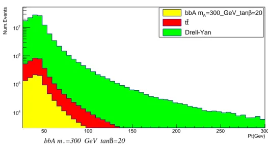
50 100 150 200 250 300 Pt(Gev) 4 10 5 10 6 10 7 10 Num.Events Muon Pt distribution =20 β =300_GeV_tan A bbA m t t Drell-Yan =20 β =300_GeV_tan A bbA m Muon Pt distribution

Figure 4.2: pT distribution of single muons (signal events with tanβ=20 hypothesis). are selected if they have at least two oppositely charged Tight muons, and they must have:

• pT>26GeV and η< 2.4

(38)

• at least one muon firing the IsoMu24 or the IsoTkMu24 trigger (because at least one of the two muons must have a pT> 24 GeV)

Furthermore, in order to avoid anomalies due to systematic errors in the simulation phase of the samples, it is required that the muon pairs have an invariant mass between 200 and 400 GeV.

The muons from the same event are merged into a dynamic array (vector) of TLorentzVector objects:

vector<TLorentzVector> tight_muons;

TLorentzVector mu;

mu.SetPtEtaPhiM(Mu_pt->at(i), Mu_eta->at(i), Mu_phi->at(i), muPDG); tight_muons.push_back(mu);

the events with at least two isolated tight muons are selected.

Instead, dynamic inclusive information of the selected events (i.e. the dynamics centre of mass information of the two muons: invariant mass, pulse and transverse pulse, η, ϕ) is saved.

Since the events with at least one b-tagged jet provide the highest sensitivity for

0 0.1 0.2 0.3 0.4 0.5 0.6 0.7 0.8 0.9 1 1 10 2 10 3 10 4 10 Bdisc_Distribution =20 β =300_GeV_tan A bbA m t t Drell-Yan =20 β =300_GeV_tan A bbA m Bdisc_Distribution

Figure 4.3: Distribution of the bdisc variable, which is used to recognize b-tagged jets,

imposing that b_disc>0.8484.

the b associated production channel, and those without b-tagged jets provide the best sensitivity for the gluon fusion production channel, the events are divided in two exclusive categories according to the presence of jets from b-quarks. This is done requiring the presence of one jet coming from the hadronization of a b-quark, b-jet. For this analysis, a b-jet is tagged using the medium working point of the CSSV2 algorithm [23], bdisc<0.8484 .

(39)

4.3. THE CUT-BASED ANALYSIS

4.3.2 Control plots

Once the exclusion and categorization phase is over, the collected dynamic information can provide a valid control tool, which can be compared with the results obtained in the reference analysis, but more generally with the data collected by the experiment CMS during the Run2 of LHC.

However, this operation is far from obvious; it is not possible to add the contri-butions of the single signal and background samples directly, because they do not correspond to the same collected statistics: the number of signal events is very overestimated, while the background is underestimated. It is therefore necessary to find multiplicative factors that establish the weights with which to combine the various samples, normalizing everything to the Luminosity (formula1.1 in sec. 1.1) of the Run2 data (L = 35861.7pb−1 _tab. _4.1_).

MC Samples Event rate R Scale factor

Drell–Yan 28968252 7.13687

ttbar 14529280 0.211419

MSSM bbA HiggsToMuMu MA 300 118201 0.0537925

Table 4.3: Scale factor as a function of the event rate and the cross section. Knowing the event rate Ri and the cross section σi (shown in table 4.2) we calculate the scale factors Wi as

Wi = L · σi

Ri ; (4.1)

in table4.3 the calculated results are shown.

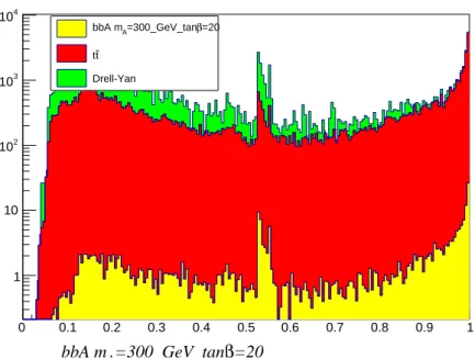
0 200 400 600 800 1000 1200 1400 mass (GeV) 1 10 2 10 3 10 4 10 5 10 6 10 7 10 events =20 β =300_GeV_tan A bbA m t t Drell-Yan =20 β =300_GeV_tan A bbA m

Mass Inclusive pre Mass Cut

0 200 400 600 800 1000 1200 1400 Mass(GeV) 10 2 10 3 10 4 10 Num.Events

Mass Inclusive post Mass Cut

=20 β =300_GeV_tan A bbA m t t Drell-Yan

Figure 4.4: Invariant mass distributions of the simulated samples.

Plots in figures 4.2, 4.3, 4.4, 4.5 are normalized using the procedure previously described; other graphs showing the distributions of some dynamic observables are

(40)

shown in appendix B.

From the plots in fig. 4.5 we see that in the case of b-tagged events, the major background is from top pair production. However, the observed b-tagged jet multiplicity for t¯t is higher than for the Higgs signal, so to improve the selection we could have rejected events with two or more b-tagged jets without affecting signifiantly the signal efficiency. Signal events are characterized by a rather small

0 20 40 60 80 100 120 140 160 180 200 2 − 10 1 − 10 1 10 2 10

Pt MEt of b-tagged event

0 20 40 60 80 100 120 140 160 180 200 1 10 2 10 3 10

Pt MEt of non b-tagged event

Figure 4.5: Evaluation of E_Tmiss for b-tagged and not b-tagged events, expressed through

the associated missing transverse impulse (pmiss

T ).

intrinsic transverse missing energy. However, the background content of the two categories (b-tagged and not) is very different. For the b-tagged category it is dominated by the t¯t events, characterized by a rather large Emiss

T , while for the not-b-tagged sample, the background is mainly from Drell-Yan events, which are characterized by a Emiss

T distributed similarly to the signal. Therefore a selection on the Emiss

T value is separately tuned for the b-tagged and the non b-tagged categories. In this thesis the cut on the Emiss

T has been optimized for the b-tagged events. Comparing the graphs with those obtained in figure4.6 produced for the reference analysis, it is seen that the study here conducted satisfactorily approximates the results. Furthermore, we can see how in a more in-depth analysis it is possible (and necessary) to confront the data collected by the CMS experiment: the simulated MC samples reproduce very well those collected during Run2.

4.3.3 Significance calculation

Optimizing the cut on the Emiss

T means finding the best compromise between the signal efficiency and the background rejection. To do this we use significance

(41)

4.4. MULTIVARIATE ANALYSIS WITH TMVA 0 20 40 60 80 100 120 140 160 180 200 (GeV) miss T p 1 10 2 10 3 10 4 10 5 10 6 10 Events/10 GeV Data Z, ZZ ± , W -W + W Single t t t Drell-Yan = 300 GeV x 100 A A m (13 TeV) -1 35.9 fb CMS b-tag category 0 20 40 60 80 100 120 140 160 180 200 (GeV) miss T p 1 10 2 10 3 10 4 10 5 10 6 10 7 10 Events/10 GeV Data Z, ZZ ± , W -W + W Single t t t Drell-Yan = 300 GeV x 100 A A m (13 TeV) -1 35.9 fb CMS No-b-tag category

Figure 4.6: Results obtained in the reference analysis [3]. In this case, other background events have also been considered which make it possible to compare them with the data obtained from the CMS experiment during Run2.

defined as

S = √ S

B+ S (4.2)

where S and B are respectively the number of signal and background events passing the cut filter (Emiss

T )i 6 (ETmiss)SM ax; then we just need to find the value that

maximizes the function S(Emiss T ).

Computatively the problem is reduced to this short code:

TH1F *Significance=new TH1F("Significance",";MEt(GeV); Sign.",1000,0,200); for (int i=1;i<1000;++i)

{Nevent=bbA_mA300_Pt_MEt_Btagged->Integral(0,i); Nbkg=ttbar_Pt_MEt_Btagged->Integral(0,i)+DY_Pt_MEt_Btagged->Integral(0,i); Significance->SetBinContent(i,Nevent/sqrt(Nevent+Nbkg)); } cout<<"Sig.MAx="<<Significance->GetMaximum()<<endl; double GetMax=(Significance->GetMaximumBin()*0.200); cout<<"MAX for="<<GetMax<<endl;

The Significance (S) is calculated bin by bin, at steps of 0.200 GeV, calculating the number of signal and background events included between zero and the reference bin. At this point it is sufficient to find the absolute maximum point of the function to know where to make the cut. In figure 4.7 it can be seen that the trend of the Significance is very similar for all the hypotheses of tan(β), and that the maximum point is for pmiss

T ∼40 GeV.

4.4 Multivariate Analysis with TMVA

A multivariate approach, making simultaneous use of several physical observables with increasing of complexity, can be a convenient for this analysis. In this thesis, using TMVA (see sec. 3.2), among the several Machine Learning algorithms used for both classification and regression problems, the BDT technique (described in Section 3.2.1 in more detail) was adopted, since it is generally more reliable and also widely used in the High Energy Physics community for the signal/background